The functional linear array model
Sarah Brockhaus1, Fabian Scheipl1, Torsten Hothorn2and Sonja Greven1
1Institut f ¨ur Statistik, Ludwig-Maximilians-Universit ¨at M ¨unchen, Germany 2Institut f ¨ur Epidemiologie, Biostatistik und Pr ¨avention, Abteilung Biostatistik, Universit ¨at Z ¨urich, Switzerland
Abstract: The functional linear array model (FLAM) is a unified model class for functional regression models including function-on-scalar, scalar-on-function and function-on-function regression. Mean, median, quantile as well as generalized additive regression models for functional or scalar responses are contained as special cases in this general framework. Our implementation features a broad variety of covariate effects, such as linear, smooth and interaction effects of grouping variables, scalar and func-tional covariates. Computafunc-tional efficiency is achieved by representing the model as a generalized linear array model. While the array structure requires a common grid for functional responses, missing values are allowed. Estimation is conducted using a boosting algorithm, which allows for numerous covariates and automatic, data-driven model selection. To illustrate the flexibility of the model class we use three applications on curing of resin for car production, heat values of fossil fuels and Canadian climate data (the last one in the electronic supplement). These require function-on-scalar, scalar-on-function and function-on-function regression models, respectively, as well as additional capabilities such as robust regression, spatial functional regression, model selection and accommodation of missings. An implementation of our methods is provided in theRadd-on packageFDboost.
Key words: boosting; functional data analysis; smoothing; structured additive regression; varying co-efficient models
ReceivedSeptember 2014;revisedDecember 2014;acceptedDecember 2014
1 Introduction
Functional data analysis (Ramsay and Silverman, 2005; Ferraty and Vieu, 2006) aims at analyzing data where the observation units are functions. Often functional regres-sion models (Ramsay and Silverman, 2005) are of interest, i.e., models containing a functional response or at least one functional covariate, resulting in three types of functional regression models: scalar-on-function, scalar and function-on-function regression models. We introduce the function-on-functional linear array model (FLAM), which includes all three model types as special cases and provides a unified model class for functional regression. Compared to existing work, which typically focused
Address for correspondence: Sarah Brockhaus, Institut f ¨ur Statistik, Ludwig-Maximilians-Universit ¨at M ¨unchen, Ludwigstraße 33, D–80539 M ¨unchen, Germany.
E-mail: [email protected] Fax: (+49) 89 2180 5308
on one of the three cases, we provide three novel extensions. First, the use of general loss functions allows us to model not only the conditional mean but also the median, any quantile or any other property of the conditional distribution representable by a suitable loss function. Most existing work has focused on mean regression for functional data, but more general loss functions than the squared error loss are in particular important for robust regression models, using, e.g., the absolute error loss or the Huber loss, and for non-normal functional data. Second, our approach is able to handle a large number of covariate effects—even more than observations—and model selection. Both, large numbers of variables and variable selection are largely unaddressed in the functional data context to date. Third, we provide a common software platform for functional regression which makes use of the array structure of FLAMs to obtain computational efficiency for estimation via generalized linear array models (Currie et al., 2006). Although we assume for the FLAM that the functions are intrinsically smooth and measured on a fine grid, missing values are allowed and make estimation for sparse functional data possible, albeit at some loss of compu-tational efficiency. In addition to compucompu-tational efficiency, this unified and modular platform has the advantage of allowing for and encouraging extensions of the model class (even though many models of common interest are already implemented) and new model terms or loss functions will then be instantly available for all models covered by our framework.
A recent overview on functional regression can be found in Morris (2015). Most prior work in this area has focused on quite narrow classes of models. The proposed models are often restricted to one functional predictor without consideration of further scalar or functional covariates and minimization of a quadratic loss function. Much work has concentrated on scalar-on-function regression—also called signal regression—modelling the functional effect linearly as the scalar product of the functional predictor and a smooth coefficient function, in the context of linear models (e.g., Reiss and Ogden, 2007; James et al., 2009), generalized linear models (e.g., Marx and Eilers, 1999; M ¨uller and Stadtm ¨uller, 2005; Wood, 2011; Gertheisset al., 2013) or quantile regression models (e.g., Cardot et al., 2005; Chen and M ¨uller, 2012a). Some approaches model the effect of the functional predictor without the as-sumption of linearity (e.g., James and Silverman, 2005; M ¨ulleret al., 2013; McLean
et al., 2014; Zhuet al., 2014). A fundamentally different approach is pursued by Fer-ratyet al.(2005, 2007) who estimate scalar-on-function regression models nonpara-metrically using kernel methods, yielding predictions but no interpretable models.
For function-on-scalar regression, which can also be viewed as smooth repeated measures varying coefficient models, most approaches model the conditional mean of a functional variable in the setting of independent (e.g., Reisset al., 2010) or depen-dent data (e.g., Morris and Carroll, 2006; Diet al., 2009; Grevenet al., 2010; Chen and M ¨uller, 2012b). Staicuet al.(2012) model conditional quantiles of a functional variable as depending on the index of the response but not on covariates.
In the context of function-on-function regression, a linear effect of a functional covariate is modelled using a bivariate coefficient surface (e.g., Ramsay and Dalzell, 1991; Yao et al., 2005; Ivanescu et al., 2014). Ferraty et al. (2012) investigate a
nonparametric kernel approach and M ¨uller and Yao (2008) consider a non-linear effect of a functional covariate.
Among the most general frameworks for functional regression models are two frameworks that can deal with functional and scalar responses and the effects of several functional and scalar covariates. One pursues a Bayesian wavelet-based approach for functional regression models; see Malloy et al. (2010) for scalar re-sponses in a distributed lag model and Morris and Carroll (2006), Zhuet al.(2011) and Meyeret al.(2013) for functional responses. Zhuet al.(2011) develop a robust function-on-scalar regression model for dependent data as generalization of the model in Morris and Carroll (2006). Zhuet al. (2011) and Meyeret al.(2013) also discuss possible generalizations to other projections than wavelets. A second general framework estimates functional regression models based on additive mixed models. This approach was proposed by Goldsmithet al.(2011) for scalar responses and by Ivanescuet al.(2014) and Scheiplet al.(2014) for functional responses. Both frame-works allow random effects, scalar and functional covariates. While our framework incorporates very similar covariate effect types as these two approaches, it is the first to go beyond modelling the conditional mean and to be able to deal with a large number of covariates as well as variable selection. In particular this means that we can estimate, e.g., quantile or expectile regression models, which is impossible in the other two approaches focusing on generalized regression models. In addition, we can accommodate situations with more covariates than observations. Furthermore, the efficient array methods we use for estimation give a clear computational advantage over Scheiplet al. (2014) for increasing sample size and number of grid points per function. Another advantage of our general framework is the unified treatment of scalar and functional response models in both models and software, making it easier for new users to get familiar with both within one framework, and allowing for simpler extension of models and accompanying code for both settings simultaneously. Our implementation of FLAMs is based on a component-wise boosting algorithm. Boosting is an ensemble method that aims at optimizing a risk function by stepwise updates of the parameters of the best-fitting effect in each iteration. Every effect is represented using a so-called base-learner, which is a simple model; see for instance B ¨uhlmann and Hothorn (2007) for an introduction to boosting algorithms in a statis-tical context. We derive an appropriate loss function for functional responses based on existing loss functions for scalar responses. Boosting has some desirable proper-ties. It can handle many covariates of mixed types including categorical and metric scalar variables and their interactions in mixed specifications, as for instance linear, smooth and multidimensional effects. Additionally, we implement a base-learner for effects of functional covariates that can be combined with existing base-learners to form interaction effects of functional and scalar covariates. The number of covariates can exceed the number of observations and the covariates can be correlated. It is of large practical importance to note that boosting can also perform variable and model selection. Little work has been done to date on variable selection in functional regres-sion models. Gertheisset al.(2013) pursued variable selection in a scalar-on-function setting. Boosting was used before in functional data analysis to estimate particular regression models. In a setting with scalar response and a single functional covariate,
boosting was used for classification of a binary response (Kr ¨amer, 2006), for predic-tion of a continuous response based on kernel regression (Ferraty and Vieu, 2009) and for feature extraction (Tutz and Gertheiss, 2010). In the context of function-on-scalar regression Sexton and Laake (2012) used boosted regression trees. A drawback of boosting is its lack of formal inference, which we address by bootstrapping.
In the following we define the general FLAM and the tensor product basis representation of the effects (Section 2). In order to fit a FLAM we define a suitable loss for functional data (Section 3). We give details on the estimation using a boosting algorithm in Section 4. In Section 5, we present empirical results on simulated data to demonstrate correctness of our software implementation and provide a comparison with penalized regression models proposed by Scheiplet al. (2014). The section on applications (Section 6) contains the analysis of two data examples. We analyze data on the viscosity of resin over time depending on five experimental factors, where the aim is to control the hardening process. In a function-on-scalar regression model for the viscosity we use median regression incorporating variable selection. In the second application, spectrography data of fossil fuel samples are used to predict their calorific values using two spectral measurements (scalar-on-function regression). The online appendix contains an additional example for function-on-function regression. All analyses are fully reproducible as the datasets and the code of the simulation and the applications are part of the online supplement or theRadd-on packageFDboost (Brockhaus, 2014) andRis open source software (R Core Team, 2014). The article concludes with a discussion in Section 7.
2 Model specification
In the following we consider data (Y, X)⊂Y×X, whereYis a suitable space for the responseY andXis a product space of suitable spaces for the covariates. LetYbe the space of square integrable functionsL2(T, ). For functional response the domainT is an interval over the real numbers,T= [t1, t2], witht1, t2∈R, andis the Lebesgue
measure. For scalar response the set Tconsists of a single point, T=[t, t], andis the Dirac measure. The spaces inXare defined analogously for scalar and functional covariates. We assume that Y given X follows a conditional distribution FY|X; the
explanatory variablesX may be fixed or random. As generic model we establish the following structured additive regression model:
(Y|X= x)=h(x)=
J
j=1
hj(x), (2.1)
where is some transformation function, for instance the expectation, the median or some quantile. For a generalized linear model the transformation function corre-sponds to the expectation composed with the link functiongthat connects response and linear predictor, i.e., =g◦E. The linear predictor h is the sum of partial ef-fects hj which implies additivity. Note, however, that a partial effecthj can depend
on more than one covariate allowing, e.g., for interactions. Each effecthj(x)∈Yis a
real valued function. To give an overview of effectshj(x) that can be specified within
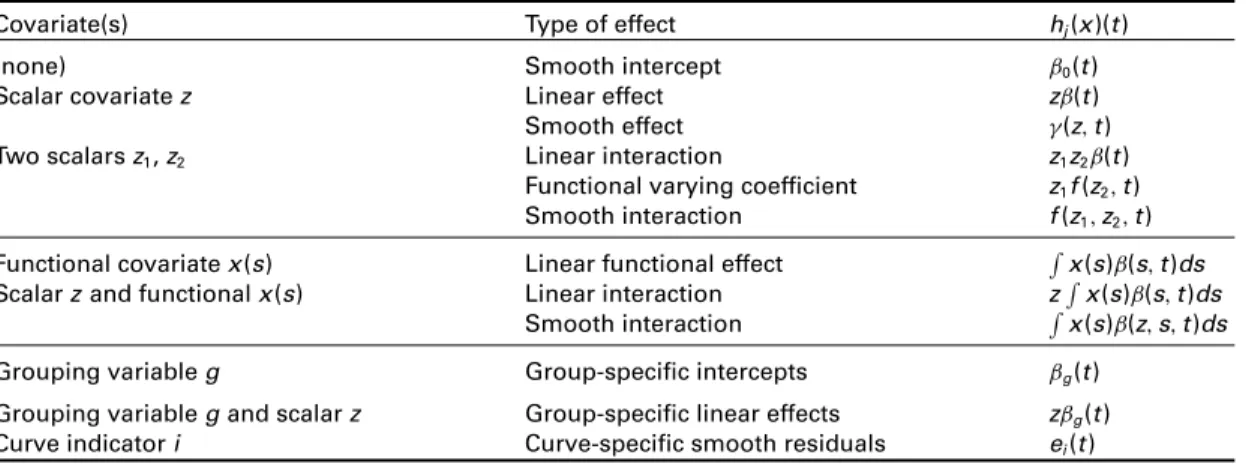
the proposed framework, Table 1 lists the effects that are currently implemented in the FDboost package (Brockhaus, 2014). A similar table can be found in Scheipl
et al.(2014). In order to obtain identifiable models, further constraints on thehj are
necessary. For an intercept ˇ0 in the model, we centre all effectshj, which contain
an intercept as a special case, by assuming that the expectation over the covariates is zero onT, i.e., EX(hj(X))≡ 0. We describe these constraints and how to include
them in the array framework in the online appendix A. Eachhj(x) is represented using a tensor product basis
hj(x)(t)=
bj(x)⊗bY(t)
j, (2.2)
where ⊗ is the Kronecker product, bj :X→RKj is a vector of basis functions
de-pending on one or several covariates,bY :T→RKY is a vector of basis functions over
the domain of the response and j ∈RKjKY is a vector of coefficients. In the case of
scalar-on-function regression,bY(t)≡1 withKY =1. Regularization of the effects is
achieved by a quadratic penalty term. A suitable penalty matrix for a tensor product basis as in equation (2.2) can be constructed as PjY =j(Pj⊗IKY)+Y(IKj ⊗PY),
where Pj ∈RKj×Kj is an appropriate penalty matrix for the marginal basis bj(xi),
PY ∈RKY×KY is an appropriate penalty matrix for the marginal basisbY(t), and j,
Y ≥0 are the corresponding smoothing parameters (Wood, 2006, sec. 4.1.8). Other
penalty matrices are possible, e.g., the direct Kronecker product of the two marginal penaltiesP∗jY =jPj⊗PY (Wood, 2006, sec. 4.1.8) or the penalty of the
sandwich-smoother P∗∗jY =jPj⊗BYBY+YBj Bj⊗PY+jYPj⊗PY, where Bj and BY are
the design matrices of the marginal bases (Xiaoet al., 2013). The penalty term has
Table 1 Basic effects that can be fitted within a FLAM.
Covariate(s) Type of effect hj(x)(t)
(none) Smooth intercept ˇ0(t)
Scalar covariatez Linear effect zˇ(t)
Smooth effect (z, t)
Two scalarsz1,z2 Linear interaction z1z2ˇ(t)
Functional varying coefficient z1f(z2, t)
Smooth interaction f(z1, z2, t)
Functional covariatex(s) Linear functional effect x(s)ˇ(s, t)ds
Scalarzand functionalx(s) Linear interaction zx(s)ˇ(s, t)ds
Smooth interaction x(s)ˇ(z, s, t)ds
Grouping variableg Group-specific intercepts ˇg(t)
Grouping variablegand scalarz Group-specific linear effects zˇg(t)
Curve indicatori Curve-specific smooth residuals ei(t)
a quadratic form, resulting in a Ridge-type penalty. The description of bases and suitable penalty matrices corresponding to the effectshj(x) in Table 1 are deferred to
Section 6, as we hope that concrete examples improve readability of these technical details. The three examples in Section 6 and the online appendix are chosen in particular such that bases and penalties for most effect types in Table 1 are introduced. As we represent all effects as Kronecker products of two bases and use a Ridge-type penalty, the model is a special case of a generalized linear array model as introduced by Currieet al.(2006). This approach in particular avoids rearranging responses and coefficients into vectors, but preserves the array structure throughout and makes use of the special Kronecker structure in the design matrix to reduce computations to nested operations in lower dimensions. For instance, it is not necessary to actually compute and save theNG×KjKY design matrix, whereNis the number of
observa-tion units andGis the number of observation points per functional response. Instead we only need to compute and save the much smaller marginal basis matrices. By defin-ing suitable array-based linear algebra routines the number of operations required to compute effect estimates and predictions, as well as the storage requirements, are reduced dramatically (cf. Currieet al., 2006).
3 Estimation
The basic idea for the estimation of a FLAM (2.1) is the use of an adequate loss function that represents the estimation problem. The choice of the loss function depends on the transformation function and on the conditional distribution of the response. In the following, we present some possible loss functions to give an idea of the variety of models that can be represented within this framework. Let
: (Y×X)×H→L1(T, ) be a function mapping the data (Y, X) and the modelh
to a function in the space of integrable functionsL1(T, ). The modelhis an element
of the set H=Y(X×T), which is the set of all functions from (X×T) to Y. In other words,maps the data and the model to a function over the domain of the response which computes a measure of discrepancy betweenY(t) andh(X)(t) for eacht∈T. For clarity, the argument t is omitted in the following examples of loss functions. For a continuousY, a typical choice is the squared error loss, the so-called L2-loss, L2
(Y, X), h= 12(Y −h(X))2. Minimizing the quadratic loss corresponds to least
squares optimization and is equivalent to minimizing the negative log-likelihood of a normal distribution. Thus minimizing theL2-loss yields the classical linear regression
model for conditionally normally distributed response and corresponds to the case when the transformation function is the expectation.
One possibility to obtain a more robust model is to use the absolute loss, also called
L1-loss, which is equivalent to minimizing the negative log-likelihood of the Laplace
distribution and is defined asL1
(Y, X), h= |Y −h(X)|. TheL1-loss is minimized
by the conditional median and hence corresponds to median regression. To obtain quantile regression, i.e., (Y|X)=Q(Y|X), where Q(Y|X) is the -quantile of Y
conditional on X for a given quantile ∈(0,1), one can use the check function (Koenker, 2005) (Y, X), h= (Y −h(X)), ifY−h(X)≥0 (Y −h(X))(−1),ifY−h(X)< 0,
which is minimized by the -quantile. Modelling quantiles is a distribution-free approach and is often of interest for skewed and heteroskedastic conditional distributions or in applications where some extreme quantile is of special interest.
If it is assumed that the conditional distribution of the response is from the expo-nential family, the negative log-likelihood is an appropriate loss function. Examples for exponential family distributions used for generalized linear models (GLMs) in-clude binomial, Poisson, log-normal and Gamma distributions (Nelder and Wedder-burn, 1972).
We define the loss function: (Y×X)×H→Rthat results in a real valued loss by integrating the loss function
(Y, X), h=
(Y, X), hd. (3.1)
Remember thatis the Dirac measure for scalar response and the Lebesgue measure for functional response. Weight functions can be incorporated by defining d(t)=
v(t)dt wherev(t)> 0 fort∈T andv(t)=0 fort∈/T, e.g.,v(t)= I(t∈T), withI the indicator function. Weight functions that are not constant can be used in case a certain area ofTis of special interest or variability varies alongT.
4 Boosting
The FLAM (2.1) could be fitted using different approaches, e.g., by penalized likelihood-based methods or Bayesian methods, replacing penalties with priors. We chose to use boosting as it can easily deal with both the diversity of possible loss functions of interest as well as with a large number of covariates (potentially more than observations) and variable selection. Boosting is an ensemble method that pursues a divide-and-conquer strategy for optimizing an expected loss criterion. The estimator is updated step-by-step to minimize the loss criterion as defined in (3.1) along the steepest gradient descent. The model is represented as the sum of simple (penalized) regression models, the so-called base-learners, that fit the negative gradient in each step (Friedman, 2001; B ¨uhlmann and Hothorn, 2007). The base-learners determine the type of possible covariate effects. Their parametrization for the FLAM (2.1) is given in equation (2.2). The loss criterion determines which characteristic of the response variable’s conditional distribution is the goal of optimization. The loss function is assumed to be differentiable with respect to h.
The aim of boosting is to find the solution of the optimization problem
h∗= argmin
h
EY,X(Y, X), h. (4.1)
In practical problems the expectation in equation (4.1) has to be replaced by the ob-served mean and the integral in equation (3.1) has to be approximated by the weighted sum over the observed points, giving optimization of the empirical risk. We consider a random sample (Yi, Xi),i=1, . . . , N, whereYi ∼FY|Xi follow a common
distribu-tion andXi can be fixed or random. We assume that the responsesYi are observed
over a common grid (t1, . . . , tG)∈T. Then we use the empirical risk for optimization
h∗ =argmin h (GN)−1 N i=1 G g=1 wii(tg) (Yi, Xi), h (tg),
where wi are weights for the observations and i(tg) are integration weights. The
weightswi are used in resampling methods, e.g., bootstrapping or subsampling, and
are set to one for an ordinary model fit. The integration weightsi(tg) are weights of
a numerical integration scheme. As a default, Riemann sums are used. In the case of a missing valueYi(tg), the corresponding weighti(tg) is set to zero and the integration
weights of adjacent observationsi(tg−1),i(tg+1) are increased accordingly. If
in-cludes a weight function, the integration weights are pre-multiplied byv(tg) at eachtg.
We adapt the component-wise boosting algorithm developed by Hothorn et al.
(2013) to estimate conditional transformation models for the case of functional regression models. In detail, we use the following algorithm to estimate FLAMs, as defined in equation (2.1).
Algorithm: Boosting for Functional Linear Array Models
1. Define the bases bj(x), bY(t), their penalties PjY,j= 1, . . . , J, and the weights
˜
wig =wii(tg),i= 1, . . . , N,g=1, . . . , G. Initialize the parameters[0]j forj=
1, . . . , J. Select the step-length ∈(0,1) and the stopping iterationmstop. Set the
number of boosting iterations to zero,m:=0. 2. Compute the negative gradient of the empirical risk
Ui(tg) := − ∂ ∂h (Yi, Xi), h (tg) h=hˆ[m] , with ˆh[m](x i)(tg)= Jj=1 bj(xi)⊗bY(tg) [jm]. Fit the base-learners forj=1, . . . , J:
ˆ j =argmin ∈RKjKY N i=1 G g=1 ˜ wig{Ui(tg)−(bj(xi)⊗bY(tg))}2+PjY,
with weights ˜wig and penalty matricesPjY.
Select the best base-learner:
j= argmin j=1,...,J N i=1 G g=1 ˜ wig{Ui(tg)− bj(xi)⊗bY(tg) ˆ j}2.
3. Update the parameters[jm +1] =
[m]
j + ˆj and keep all other parameters fixed,
i.e.,[jm+1]=j[m], forj=/ j.
4. Unlessm=mstop, increasemby one and go back to step 2.
Then the final model is: ˆ (Yi|Xi =xi)= J j=1 ˆ h[mstop] j (xi), with ˆh[mstop] j (xi)(t)= bj(xi)⊗bY(t) [mstop] j .
To complete the specification of the boosting algorithm, it is necessary to set all parameters mentioned in step 1. The bases and their corresponding penalty matrices directly correspond to the chosen partial effectshj(x) in the model, with an overview
of possible model terms given in Table 1 and various examples of choices for bases and penalties discussed in Section 6. Obvious choices are splines for smooth terms and the observations themselves for linear terms, in each case provided with adequate penalty matrices. We used a simplified penalty matrixPjY = j(Pj⊗IKY +IKj ⊗PY)
which contains only one smoothing parameter for both directions in our implementa-tion. Additional simulations (results not shown) indicate that the effect estimates still adapt well to anisotropic effect surfaces over the course of the boosting iterations. The smoothness parametersj are chosen such that the degrees of freedom are the
same for all base-learners to ensure a fair model selection. Otherwise base-learners with higher degrees of freedom are more likely to be chosen (Hofner et al., 2011). The resulting estimates adapt to the true complexity of the effects by the selection frequency of the base-learners, which depends on the number of boosting iterations
mstop (B ¨uhlmann and Yu, 2003). A natural choice for all initial values [0]j is zero.
However, the convergence rate of the boosting algorithm is faster if a suitable offset is chosen for the intercept. For scalar responses typical choices are mean or median. For functional responses, we use a smoothed mean or median function as offset.
The number of boosting iterations mstop and the step-length are connected, as
a smaller length typically requires more boosting iterations. Choosing the step-length sufficiently small (e.g., =0.1) and using the number of boosting iterations as tuning parameter has been shown to be a good strategy (Friedman, 2001). Stopping early here leads to regularized effect estimates and the number of boosting iterations
mstop can be chosen by resampling methods like cross-validation or bootstrapping.
If bootstrapping is used, the weights wi are drawn from an N-dimensional
multi-nomial distribution with constant probability parameters pi =N−1, i=1, . . . , N.
Then the out-of-bootstrap (OOB) empirical risk with weights wOOBi =I(wi =0) is
computed and the stopping iteration yielding the lowest empirical risk is chosen (Hothornet al., 2013).
Stability selection (Meinshausen and B ¨uhlmann, 2010) can be used to improve variable selection. The basic idea is to fix an upper bound for the per-family-error-rate and the expected number of terms in the model. Then the model is refitted on sub-samples of the data and the stability selection procedure provides a cutoff value for the relative frequency of a base-learner to be selected among the first model terms across the subsamples. Terms with selection frequencies greater than the cutoff are retained in the model. In this article we use complementary pairs stability selection as proposed by Shah and Samworth (2013), which improves on the theoretical guarantees of the original proposal of Meinshausen and B ¨uhlmann (2010) by replacing purely ran-dom subsampling of the data with subsampling consisting of complementary pairs— for each subsample of size N/2 another subsample containing the observations not used in that subsample, i.e., the complementary pair, is also used as a training subsample.
5 Simulation study
The aim of the simulation study is to demonstrate correctness of our software implementation in theRadd-on packageFDboost(Brockhaus, 2014). Details on the construction of the base-learner for a functional covariate are given later in Section 6.2. Boosting for scalar responses and covariates is well tested and extensive simula-tion studies have already been conducted for theRadd-on packagemboost(Hothorn
et al., 2014) on which our implementation is based (e.g., B ¨uhlmann and Hothorn, 2007; Schmid and Hothorn, 2008; Fenske et al., 2011). To keep the simulation section short, we use a function-on-function setting which covers the functional response and the functional covariate setting—both new in our framework—at the same time. To allow comparison with a benchmark we simulate a mean regression model, i.e., =E, with a moderate number of covariates and no need for variable se-lection. We can then use penalized function-on-function regression (PFFR) proposed by Ivanescuet al.(2014) and Scheiplet al.(2014) and implemented in theRadd-on package refund (Crainiceanu et al., 2014) as a benchmark. Scheipl et al. (2014) demonstrated in the function-on-scalar setting that the PFFR approach is better suited to smooth functional data—as we assume—than the Bayesian wavelet-based approach by Morris and Carroll (2006). The effect of the functional covariates in both approaches is specified using the default settings, which means that a tensor product of cubic regression splines is used in PFFR and cubic P-splines are used in the boosting algorithm. For the boosting algorithm of the FLAM, the optimalmstop
Simulation set-up and goodness of fit measure. We consider a model with func-tional response and two funcfunc-tional covariates. The true model is
Yi(t)= ˇ0(t)+
x1i(s)ˇ1(s, t)ds+
x2i(s)ˇ2(s, t)ds+εit,
with s, t∈[0,1]. The functional covariates are simulated using a sum of five natu-ral cubic B-splines with random coefficients from a uniform distribution U[−3,3]. The smooth global intercept isˇ0(t)=cos(3t2)+2, the coefficient functionˇ1(s, t)
is a bimodal surface ˇ1(s, t)=(s, .2, .3)(t, .2, .3)+(s, .6, .3)(t, .8, .25), where (·, , ) is the density of the normal distribution with mean and standard de-viation, and the coefficient functionˇ2(s, t) is unimodal withˇ2(s, t)=1.5 sin(t+
0.3) sin(s). The errors are normally distributed withεit ∼N(0, ε2), whereε2depends
on the signal-to-noise ratio. In the online appendix B a figure of the true coefficient functions and responses together with the estimates by PFFR and FLAM is given for an exemplary setting. We consider all combinations of the following parameter settings:
1. total number of observationsN ∈ {100,500}
2. number of grid pointsG∈ {30,100}; the same number of grid points is used for response and functional covariates
3. signal-to-noise ratio SNRε ∈ {1,2}, where SNRε is the ratio of the standard
deviation of the linear predictor and the standard deviation of the residuals. We run 10 replications per combination of parameter settings, which results in narrow interquartile ranges of the performance measures and thus seems sufficient. As a measure of the goodness of estimation, the relative integrated mean squared error (reliMSE) is used:
reliMSE(Y(t)) = N i=1 i(t)−Yˆi(t) 2 dt N i=1 i(t)−Y¯ 2 dt
where i(t) is the true value of the response without noise, ˆYi(t) is the predicted
value and ¯Y =N−1 i
i(t)dt is the global mean of the response. Thus, the mean
squared error (MSE) is standardized with respect to the global variability of the response. The reliMSE is calculated analogously for the coefficient surfaceˇ(s, t):
reliMSE(ˇ(s, t)) =
ˇ(s, t)−ˇˆ(s, t)2dsdt,
ˇ(s, t)−ˇ¯2dsdt
whereˇ(s, t) is the true coefficient surface, ˆˇ(s, t) is its estimate and ¯ˇ= ˇ(s, t)dsdt
the global variability of the coefficient surface. The reliMSE is defined analogously for the univariate coefficient functionˇ0(t).
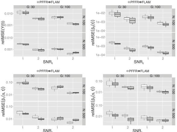
Simulation results. A graphical analysis of results (Figure 1) shows that the accu-racy of estimates for the functional effects as well as the prediction of the response using boosting is quite similar to that obtained when estimating the models with PFFR. The reliMSE depends mainly on the signal-to-noise ratio SNRε and the
num-G: 30 G: 100 ● ● ● 0.001 0.010 0.001 0.010 N: 100 N: 500 1 2 1 2 SNRε reliMSE(Y(t)) PFFR FLAM G: 30 G: 100 ● ● ● ● ● ● 1e−04 1e−03 1e−02 1e−04 1e−03 1e−02 N: 100 N: 500 1 2 1 2 SNRε reliMSE ( β0 ( t )) PFFR FLAM G: 30 G: 100 ● ● ● ● ● 0.01 0.10 0.01 0.10 N: 100 N: 500 1 2 1 2 SNRε reliMSE ( β1 ( s , t )) PFFR FLAM G: 30 G: 100 ● ● ● 0.01 0.10 0.01 0.10 N: 100 N: 500 1 2 1 2 SNRε reliMSE ( β2 ( s , t )) PFFR FLAM
Figure 1 Simulation results. The upper left panel shows the reliMSE for the prediction of the response, the upper right panel the reliMSE for the smooth intercept and the two lower panels show the reliMSE for the two
functional effects for all combinations of sample sizeN, number of grid pointsGand signal-to-noise ratio
SNRε.
Source:Authors’ own.
ber of observation points per curveG. As expected, the estimates and predictions are better for higher signal-to-noise ratio, more observations per curve and a higher num-ber of observed curves. The estimates ofˇ2(s, t) are generally better than the estimates
ofˇ1(s, t), which can be explained by the more complex bimodal shape of the latter.
As the reliMSE is similar for PFFR and FLAM, showing no preference for one of the two methods, one can assume that the new boosting algorithm is up to the standard
of the benchmark for those cases where the benchmark is applicable, while consider-ably extending the class of possible models. The computation time of the models in all the considered settings and for both algorithms ranges from some seconds up to 10 minutes. To compute the computation time for the FLAM, we parallelized the 10-fold bootstrap on 10 cores. For the relatively small data situations considered in the simu-lation (small samples size, few observations per curve, only two effects), PFFR is faster, but FLAM scales better for a growing number of observations and more covariates and is faster for the setting withN = 500 andG =100 (see online appendix B). 6 Applications
In this section, we present analyses for scalar-on-function and function-on-scalar regressions, giving exemplary choices of transformation functionsand base-learners forhj(xi) to illustrate some possibilities of the generic model (2.1). Online appendix
C contains an additional example for function-on-function regression, together with a comparison with the PFFR approach of Scheiplet al.(2014). In addition to base-learners for scalar and functional covariates and their interactions, the three examples require robust (median) regression, variable selection and the handling of missing values and spatially correlated functional residuals.
6.1 Function-on-scalar regression: viscosity
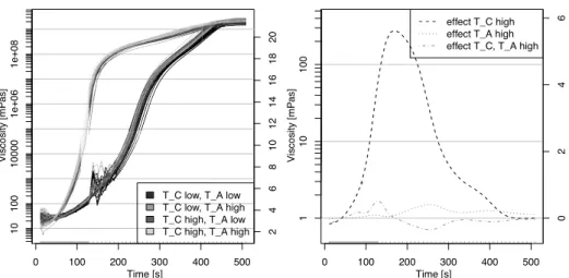
In the fabrication of cars, casting is an important production technology. For this process the curing of the material, in our example resin, in the mould is crucial. To determine factors that affect curing, the viscosity of the resin is measured over time in an experiment varying five binary factors (Wolfgang Raffelt, Technical Univer-sity of Munich, Institute for Carbon Composites). The ideal viscoUniver-sity-curve should have low values in the beginning and then increase quickly. This corresponds to low viscosity during filling of the mould and a rapid hardening. Following a fractional factorial design, 16 factor combinations were tested with 4 replications per experi-mental setting. Due to technical reasons the measuring method has to be changed in a certain range of viscosity. As the time-point for the change of measuring method is at 109 seconds for some curves and at 129 seconds for others, there are missing values in those curves with the earlier change point due to the smaller frequency for the second method. After the change of method some curves show large amounts of measurement error. In Figure 2 the observed viscosity curves are plotted on a log-scale in micropascal. For the modelling, main effects and interactions of first order for the five experimental factors are of interest, resulting in 15 potential effects. The estimates should be robust because of the apparent measurement error problems in some curves. All in all it is necessary to estimate a robust (median) regression model, incorporating model selection and accommodating missing values. A FLAM can deal with all of these problems: Median regression is obtained by using the absolute loss, variable selection is achieved by stability selection, and missing values are dealt with by setting the corresponding weights to zero.
●●●●●●●●●●●●●●●●●●●●●●●●●●●●●●●●●●●●●●●●●●●●●●●●●●●●●●●●●●●●●●●●●●●●●●●●●●●●●●●●●●●●●●●●●●●●●●●●●● 0 100 200 300 400 500 Time [s] Viscosity [mP a s] 10 100 1 0000 1e+06 1 e+08 2468 1 0 1 2 1 4 16 18 20
T_C low, T_A low T_C low, T_A high T_C high, T_A low T_C high, T_A high
●●●●●●●●●●●●●●●●●●●●●●●●●●●●●●●●● ●●●●●●●●●●●●●●●●●●●●●●●●●●●●●●●●●● ●●●●●●●●●●●●●●● 0 100 200 300 400 500 Time [s] Viscosity [mP a s] 1 10 100 02 46 effect T_C high effect T_A high effect T_C, T_A high
Figure 2 Viscosity over time and estimated coefficient functions. On the left hand side the viscosity measures are plotted over time with temperature of tools (T C) and temperature of resin (T A) colour-coded. On the right hand side the coefficient functions are plotted.
Source:Authors’ own.
In the first step a smooth intercept, all main effects and all interaction terms of first order are included in the model as smooth effects over time. To estimate such a model we need a base-learner for an effect of the formxˇ(t), wherexis a dummy variable for a factor or an interaction andˇ(t) is the smooth coefficient function over time. Such an effect is obtained by setting bj(x) =(1 x) andbY(t)= Y(t), whereY(t)
is a vector of cubic B-splines evaluated att. The smooth intercept is represented by settingb1(x) =(1). In order to get more stable estimates and reduce the necessary
number of boosting iterations, we include an intercept term in each base-learner. After fitting the model, the intercept-part is subtracted from each coefficient function and added to the global intercept. The penalty matrixPjfor the linear term in the dummy
variable is0so that the linear term is unpenalized, and the penalty matrixPY isDD
with second-order difference matrixD, yielding P-splines for the time-varying effects (Eilers and Marx, 1996).
The optimal stopping iteration is determined by 10-fold bootstrapping over curves. In the resulting model, all main effects and most of the interaction effects are selected. Most base-learners contribute very small effects to the prediction of the viscosity and are selected quite rarely. To obtain a parsimonious model only containing important effects we conduct stability selection (Shah and Samworth, 2013). We set the per-family-error-rate to 2 and the expected number of terms in the model to 5. For the 16 possible base-learners this results in a cutoff value of 0.63. Using a total of 100 subsamples, the effects for temperature of tools (T A), temperature of resin (T C) and their interaction are selected into the model, yielding
medianlog(visi(t))|T Ai,T Ci
where visi(t) is the viscosity of observationiat timet, T Ai and T Ci are the
temper-atures of resin and of tools, respectively, each coded as -1 for the lower and 1 for the higher temperature. The interaction T ACi is 1 if both temperatures are in the higher
category and -1 otherwise. The estimated coefficients for this model are shown in Figure 2 on the right hand side.
Temperature of tools (T C) has a very strong influence. For higher temperature of tools the resin has lower viscosity in the beginning, but from about 40 seconds onwards it cures faster. For the temperature of the resin (T A), the effect is similar but much smaller, i.e., the resin cures faster for higher temperatures. If both temperatures are in the higher category the viscosity curves have the desired shape (low in the beginning and rapid increase). The other factors seem to have no or a very small influence on the curing process. This is good news for the production process, as these parameters do not have to be controlled precisely.
6.2 Scalar-on-function regression: spectral data of fuels
In this application, the aim is to predict the heat value of fossil fuels using spectral data (Fuchset al., 2015, Siemens AG). The dataset was obtained in a laboratory and contains the heat value in megajoule (MJ), percentage of humidity and two spectra types with different wavelength ranges for 129 fossil fuel samples. One spectrum is ultraviolet-visible (UV-VIS), measured at 1335 wavelengths, the other a near infrared spectrum (NIR), measured at 2307 wavelengths. The observation points along the wavelength are non-equidistant for both spectra, with larger distances for higher wavelengths.
The aim is to predict the heat value using information obtainable as measurements in a power plant, i.e., using only the spectral data. To use more information, we com-pute the derivatives of both spectra as further functional covariates. As the humidity cannot be measured automatically in a power plant, it should not be used directly for the prediction of the heat value. But it is possible to predict the humidity using the spectral data and then to use predicted humidity as additional variable. To predict the humidity we use a scalar-on-function regression model with both spectra and both derivatives as covariates. For this dataset the humidity can be predicted quite accu-rately, with the relative mean squared error (relMSE) determined by 50-fold bootstrap being about 10%. Through the predicted humidity the information contained in the spectra is used in a non-linear way for the model of the heat value. Figure 3 shows a histogram of the heat value (top left panel), whose distribution is skewed towards higher values. The scatterplot of heat value against predicted humidity (Figure 3 top right) shows that low heat values all occur for rather low humidity values, but for the low humidity values there are high heat values as well.
For this application, we want to estimate a scalar-on-function regression model that predicts the heat values as precisely as possible. Two spectra, their derivatives and the predicted humidity are available as predictors and can be used to specify models with different covariate effects. The most complex model contains the functional effects of the two spectra and their derivatives, the effect of the predicted humidity and the interaction effects of the predicted humidity with the four functional variables.
Heat value [MJ] Frequency 10 15 20 25 30 0 5 10 20 30 1 2 3 4 5 6 7 10 15 20 25 30 Predicted humidity [%] Heat v a lue [MJ] ● ● ● ● ● ● ● ● ● ● ● ● ● ● ● ● ●● ● ● ● ● ● ● ● ● ● ● ● ● ●● ● ● ● ● ● ● ● ● ● ● ● ● ● ● ● ● ● ● ● ● ● ● ● ● ● ● ● ● ● ● ● ● ● ● ● ● ● ● ●● ● ● ● ● ● ● ● ● ● ● ●● ● ●● ● ● ● ● ● ● ● ● ●● ● ● ● ● ● ● ● ● ● ● ● ● ● ● ● ● ● ● ● ● ● ● ● ● ● ● ● ● ● ● ● ● 300 500 700 900 −3 −2 −1 0 1 Wavelength [nm] UV−VIS 1000 1500 2000 2500 −1.5 −1.0 −0.5 0.0 0 .5 Wavelength [nm] NIR
Figure 3 Spectral data of fossil fuels. The colouring of all plots is according to the heat value in MJ, with red meaning low heat value and yellow meaning high heat value. The histogram at the top left can be used as a legend. The scatter plot at the top right shows the heat value depending on the predicted humidity. The lower panel shows the UV-VIS and the NIR spectra.
Source:Authors’ own.
The functional variables are denoted byxki,k=1, . . . ,4, and the predicted humidity
byzi,i= 1, . . . ,129. Then we can write the model as E(Yi|xi, zi)=ˇ0+ 4 k=1 xki(sk)ˇk(sk)dsk+f(zi)+ 4 k=1 xki(sk)˛k(sk, zi)dsk, (6.1)
whereYiare the heat values,ˇk(sk) are the coefficients of the main functional effects,
skare the respective wavelengths,f(zi) is the smooth effect of the predicted humidity
and˛k(sk, zi) are the interaction effects of the functional covariates with the predicted
humidity.
To estimate the full model (6.1), linear effects of functional variables, a smooth effect of a scalar variable and interactions between them are needed. The effect of a functional covariate x(s) over the domain s∈S is modelled asSx(s)ˇ(s)ds. The
integral can be approximated numerically as a weighted sum over (s1, . . . , sR), the
grid of observation points inS, by using adequate integration weights(s), yielding
Sxi(s)ˇ(s)ds≈ Rr=1(sr)x(sr)ˇ(sr) (Wood, 2011). Then we compute the basis as
bj(x(s)) =[ ˜x(s1)· · ·x˜(sR)] ⎡ ⎢ ⎣ j(s1) .. . j(sR) ⎤ ⎥ ⎦, (6.2)
where ˜x(s)=(s)x(s) and j(s) is a vector of B-splines evaluated at s. The penalty
matrixPjis a squared difference matrix. The smooth effectf(zi) of the scalar covariate
upon a scalar response is a standard problem and is estimated by P-splines, i.e.,
bj(z)=j(z) with difference penalty Pj. An interaction term between a functional
and a scalar variable can be computed as a tensor-product basis of the basis for the functional covariate and the basis for the scalar covariate yielding
bj(x(s), z) =bj1(x(s))⊗bj2(z),
withbj1defined as in (6.2) and thebj2(z) defined likebj(z) above. The penalty matrix
Pj for the interaction can be computed from the marginal penalties as described for
(2.2). As there is a scalar response, the basisbY(t) over the domain of the response is 1.
In order to assess the predictive power of the models we use 50-fold bootstrap and evaluate the MSE as well as the relative MSE (relMSE), which is defined as
relMSEo = i∈Io
(Yi−Yˆi)2 i∈Io(Yi −
¯
Y)2, o=1, . . . ,50,
where Io is the index set of the out-of-bag sample for bootstrap-fold o, i.e., the
validation sample, and ¯Y is the mean of the response in the learning sample. The MSE corresponds to the numerator, MSEo= i∈Io(Yi −Yˆi)2. The optimal stopping
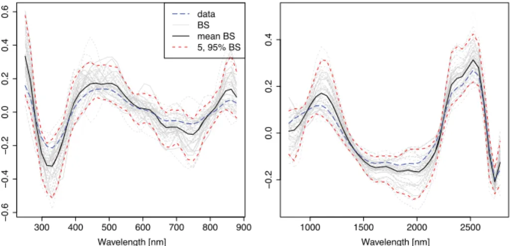
iteration is determined at the minimal mean MSE over all bootstrap samples. The predictive power of model (6.1) (fullmodel) is compared to the smaller models with all main effects ((d)spec H2O), with all functional effects ((d)spec), with both spectra (spec) and with the NIR spectra (NIR). The relMSE and the MSE for these are plotted in Figure 4. The NIR model is worse than the other models. As the model with both spectra has MSE and relMSE values close to those of the more complex models, we keep that model. The relMSE values of around 10% indicate adequate prediction of the heat values. The coefficient estimates (Figure 5) on the entire dataset (long-dashed blue lines) are plotted together with the estimates calculated on the 50 bootstrap folds (gray lines), the mean coefficient function over the bootstrap sam-ples (black lines) and point-wise 5% and 95% values over the estimated coefficient functions on the bootstrap samples (dashed red lines). The estimates are quite stable having a similar form and size over the bootstrap-samples. High values of the UV-VIS spectrum for the lowest wavelengths and low values for wavelengths of about 300
● ●
● ●
full (d)spec H2O (d)spec spec NIR
3
4567
MSE
full (d)spec H2O (d)spec spec NIR
0.10
0.15
0.20
0.25
relMSE
Figure 4 Predictive power. MSE and relMSE for models with different effects: the model with all effects (full), with all the main effects ((d)spec H2O), the effects of both spectra and their derivatives ((d)spec), the effects of both spectra (spec) and the effects of the NIR spectrum (NIR).
Source:Authors’ own.
300 400 500 600 700 800 900 −0.6 −0.4 −0.2 0.0 0 .2 0.4 0 .6 Wavelength [nm] data BS mean BS 5, 95% BS 1000 1500 2000 2500 −0.2 0.0 0 .2 0.4 Wavelength [nm]
Figure 5 Estimated coefficient functions. Coefficient estimates for the effects ˆˇj(sj),j=1,2, of the two
spectra. The gray lines show the estimates in the 50 bootstrap folds, the black line gives the mean estimated coefficient over the bootstrap folds, the dashed red lines point-wise 5% and 95% values; the long-dashed blue lines give the estimated coefficients for the model on the whole dataset.
Source:Authors’ own.
to 400 nm are associated with higher heat values. A higher spectrum in the lower wavelengths of the NIR spectrum (approximately 1000 to 1200 nm) as well as in the area of 2200 to 2600 nm are associated with a higher heat value. For the highest wavelengths and the wavelength between 1400 and 2100 nm the effect is negative, i.e., higher values in the spectrum imply lower heat values.
7 Discussion
In this article we introduced the functional linear array model (FLAM), a generic model class for functional data measured on a common grid with potential missings.
The response can be scalar or functional. The FLAM has a modular structure: the transformation function allows us to choose which feature of the conditional distri-bution of the response to model and the additive predictor allows the specification of a variety of covariate effects. We take advantage of the Kronecker product structure of the design matrix to achieve computational efficiency using linear array models. The optimization problem in (4.1) could be solved by a variety of algorithms. We decided to use a boosting approach for estimation as it is well suited to the modular structure of the model class. New base-learners can easily be implemented to adapt the modelling framework even further if new kinds of covariate effects are needed in a given problem at hand, as shown by the interaction effect between a scalar and a functional covariate in the spectral data example or the smooth spatially correlated residuals in the model for the Canadian weather data. Our current implementation includes base-learners for quite a number of common effects of scalar, functional and grouping variables and their interactions. Another attractive feature of boosting is its capability to deal with many covariate effects and to facilitate variable selection, as illustrated with the viscosity data.
Considering other general frameworks for functional regression, the mixed model based approach by Scheipl et al. (2014) and the Bayesian wavelet-based approach by Meyer et al. (2013) (and earlier work by each group), some advantages and drawbacks of FLAMs become visible. Our boosting framework is more flexible in allowing to model more general features of the response than the mean and handling the case of a large number of potential covariates. The modular framework easily allows the extension of the model class by specifying new covariate effects or loss functions. For the case of mean regression, these other two approaches naturally allow for inference as a by-product of the mixed models/Bayesian modelling frame-work. We handle the lack of formal inference using the bootstrap as illustrated with the spectral data. A table summarizing the characteristics of the three approaches is given in the online appendix D.
We are considering several future extensions to our framework. It is straightforward to implement further base-learners for additional covariate effects. One possibility would be a non-linear functional effectSf(X(s), s)ds, withfa smooth unknown function (e.g., M ¨ulleret al., 2013; McLean et al., 2014), where the basis and penalty specification of McLean et al. (2014) could be directly translated to a new base-learner. Another is to use a different set of basis functions in the estimation of linear functional effects. For instance, one could use the eigenfunctions of the es-timated covariance function as basis functions forbY(t), as is commonly done in the
context of functional principal component analysis (e.g., Scheiplet al., 2014). Another interesting future direction would be to use boosting for functional regression models that cannot be written as linear array models. This would allow for responses observed on irregular grids and for functional effects whose integration limits depend on the current observation point of the response. For instance, if functional response and covariate are observed over time, the histor-ical functional linear model (Malfait and Ramsay, 2003; Harezlak et al., 2007)
(Y(t)|X =x)=tt−ıx(s)ˇ(s, t)dscan be of interest, where only lagged past values of the functional covariate are used to model the current value of the response.
Acknowledgements
We acknowledge support from the German Research Foundation through Emmy Noether grant GR 3793/1-1 (SB, FS, SG). Special thanks to Benjamin Hofner for his advice on stability selection. Thanks to Wolfgang Raffelt for providing us with the viscosity data and to the Siemens AG for the spectral data of fossil fuels. We thank the referees and the editor for their useful comments.
References
Brockhaus S (2014)FDboost: boosting functional regression models. R package version 0.0-7. Available at http://r-forge.r-project.org/ projects/fdboost/.
B ¨uhlmann P and Hothorn T (2007) Boosting algo-rithms: regularization, prediction and model fitting (with discussion). Statistical Science, 22, 477–505.
B ¨uhlmann P and Yu B (2003) Boosting with the L2 loss: regression and classification. Journal of the American Statistical Association,98, 324–39.
Cardot H, Crambes C and Sarda P (2005) Quantile regression when the covariates are functions. Nonparametric Statistics, 17, 841–56.
Chen K and M ¨uller H-G (2012a) Conditional quantile analysis when covariates are func-tions, with application to growth data. Journal of the Royal Statistical Society: Se-ries B (Statistical Methodology),74, 67–89. Chen K and M ¨uller H-G (2012b) Modeling re-peated functional observations. Journal of the American Statistical Association, 107, 1599–609.
Crainiceanu CM, Reiss P, Goldsmith J, Huang L, Huo L, and Scheipl F (2014) refund: re-gression with functional data. R package version 0.1-11. Available at http://CRAN.R-project.org/package=refund.
Currie ID, Durban M and Eilers PHC (2006) Gen-eralized linear array models with applica-tions to multidimensional smoothing. Jour-nal of the Royal Statistical Society: Series B (Statistical Methodology),68, 259–80. Di C-Z, Crainiceanu CM, Caffo BS and
Punjabi NM (2009) Multilevel functional
principal component analysis. The Annals of Applied Statistics,3, 458–88.
Eilers PHC and Marx BD (1996) Flexible
smoothing with B-splines and penalties (with comments and rejoinder). Statistical Science,11, 89–121.
Fenske N, Kneib T and Hothorn T (2011) Identifying risk factors for severe child-hood malnutrition by boosting additive
quantile regression. Journal of the
American Statistical Association, 106, 494–510.
Ferraty F, Rabhi A and Vieu P (2005) Conditional quantiles for dependent functional data with application to the climatic El Ni ˜no phenomenon.Sankhy ¯a: The Indian Journal of Statistics,67, 378–98.
Ferraty F and Vieu P (2006) Nonparametric
functional data analysis. Springer Series in Statistics. Springer, New York. Theory and practice.
Ferraty F and Vieu P (2009) Additive prediction and boosting for functional data. Com-putational Statistics & Data Analysis, 53, 1400–13.
Ferraty F, Mas A and Vieu P (2007)
Non-parametric regression on functional data: inference and practical aspects. Australian & New Zealand Journal of Statistics, 49, 267–86.
Ferraty F, Van Keilegom I and Vieu P (2012) Regression when both response and predic-tor are functions. Journal of Multivariate Analysis,109, 10–28.
Friedman JH (2001) Greedy function approxi-mation: a gradient boosting machine. The Annals of Statistics,29, 1189–232.
Fuchs K, Scheipl F and Greven S (2015) Penal-ized scalar-on-functions regression with interaction term. Computational Statistics & Data Analysis,81, 38–51.
Gertheiss J, Maity A and Staicu A-M (2013) Variable selection in generalized functional linear models.Stat,2, 86–101.
Goldsmith J, Bobb J, Crainiceanu CM, Caffo B and Reich D (2011) Penalized functional regression. Journal of Computational and Graphical Statistics,20, 830–51.
Greven S, Crainiceanu CM, Caffo B and Reich D (2010) Longitudinal functional principal component analysis. Electronic Journal of Statistics,4, 1022–54.
Harezlak J, Coull BA, Laird NM, Magari SR and Christiani DC (2007) Penalized solutions to functional regression problems. Com-putational Statistics & Data Analysis,51, 4911–25.
Hofner B, Hothorn T, Kneib T and Schmid M (2011) A framework for unbiased model selection based on boosting. Journal of Computational and Graphical Statistics, 20, 956–71.
Hothorn T, Kneib T and B ¨uhlmann P (2013) Conditional transformation models. Jour-nal of the Royal Statistical Society: Series B (Statistical Methodology),76, 3–27. Hothorn T, B ¨uhlmann P, Kneib T, Schmid M
and Hofner B (2014)mboost: model-based boosting. R package version 2.3-0. Available at http://CRAN.R-project.org/ package=mboost.
Ivanescu AE, Staicu A-M, Scheipl F and Greven S (2014) Penalized function-on-function reg-ression. Computational Statistics. In press, DOI 10.1007/s00180-014-0548-4.
James GM and Silverman BW (2005) Functional
adaptive model estimation. Journal of
the American Statistical Association, 100, 565–76.
James GM, Wang J and Zhu J (2009) Functional linear regression that’s interpretable. The Annals of Statistics,37, 2083–108.
Koenker R (2005) Quantile regression.
Cam-bridge: Cambridge University Press.
Kr ¨amer N (2006) Boosting for functional
data. In Alfredo R and Maurizio V (eds),
COMPSTAT: Proceedings of the 17th International Conference on Computa-tional Statistics, pp. 1121–28. Heidelberg: Physica-Verlag.
Malfait N and Ramsay JO (2003) The historical functional linear model. Canadian Journal of Statistics,31, 115–28.
Malloy EJ, Morris JS, Adar SD, Suh H, Gold DR and Coull BA (2010) Wavelet-based func-tional linear mixed models: an application to measurement error-corrected distributed lag models. Biostatistics,11, 432–52. Marx BD and Eilers PHC (1999) Generalized
linear regression on sampled signals and curves: a P-spline approach.Technometrics, 41, 1–13.
McLean MW, Hooker G, Staicu A-M, Scheipl
F and Ruppert D (2014) Functional
generalized additive models. Journal of Computational and Graphical Statistics,23, 249–69.
Meinshausen N and B ¨uhlmann P (2010) Stability selection. Journal of the Royal Statistical Society: Series B (Statistical Methodology), 72, 417–73.
Meyer MJ, Coull BA, Versace F, Cinciripini P and Morris JS (2013) Bayesian function-on-function regression for multi-level functional data. Technical report, The Selected Works of Jeffrey S. Morris. Avail-able at http://works.bepress.com/jeffrey s morris/52.
Morris JS (2015) Functional regression anal-ysis. Annual Review of Statistics and its Applications,2. In press.
Morris JS and Carroll RJ (2006) Wavelet-based functional mixed models. Journal of the Royal Statistical Society: Series B (Statistical Methodology),68, 179–99.
M ¨uller H-G and Stadtm ¨uller U (2005) General-ized functional linear models. The Annals of Statistics,33, 774–805.
M ¨uller H-G and Yao F (2008) Functional additive models. Journal of the American Statistical Association,103, 1534–44.
M ¨uller H-G, Wu Y and Yao F (2013)
Con-tinuously additive models for nonlinear functional regression. Biometrika, 100, 607–22.
Nelder JA and Wedderburn RWM (1972) Gener-alized linear models. Journal of the Royal Statistical Society: Series A (Statistics in Society),135, 370–84.
R Core Team (2014) R: a language and
en-vironment for statistical computing. R
Foundation for Statistical Computing,
Vienna, Austria. R 3.1.0. Available at
http://www.R-project.org/.
Ramsay JO and Dalzell CJ (1991) Some tools for functional data analysis (with discussion). Journal of the Royal Statistical Society: Series B (Statistical Methodology), 53, 539–72. With discussion and a reply by the authors.
Ramsay JO and Silverman BW (2005)Functional data analysis. New York: Springer-Verlag. Reiss PT and Ogden RT (2007) Functional
prin-cipal component regression and functional partial least squares. Journal of the Amer-ican Statistical Association,102, 984–96. Reiss PT, Huang L and Mennes M (2010) Fast
function-on-scalar regression with penal-ized basis expansions. The International Journal of Biostatistics,6, 1–30.
Scheipl F, Staicu A-M, and Greven S (2014)
Functional additive mixed models.
Journal of Computational and Graph-ical Statistics. In press, DOI 10.1080/ 10618600.2014.901914.
Schmid M and Hothorn T (2008) Boosting
additive models using component-wise P-splines.Computational Statistics & Data Analysis,53, 298–311.
Sexton J and Laake P (2012) Boosted coefficient models. Statistics and Computing, 22, 867–76.
Shah RD and Samworth RJ (2013) Variable
selection with error control: another look
at stability selection. Journal of the Royal Statistical Society: Series B (Statistical Methodology),75, 55–80.
Staicu A-M, Crainiceanu CM, Reich DS and
Ruppert D (2012) Modeling functional
data with spatially heterogeneous shape characteristics.Biometrics,68, 331–43. Tutz G and Gertheiss J (2010) Feature extraction
in signal regression: a boosting technique for functional data regression. Journal of Computational and Graphical Statistics, 19, 154–74.
Wood SN (2006) Generalized additive models: a introduction with R. Boca Raton, Florida: Chapman & Hal/CRC.
Wood SN (2011) Fast stable restricted maximum likelihood and marginal likelihood estima-tion of semiparametric generalized linear models. Journal of the Royal Statistical Society: Series B (Statistical Methodology), 73, 3–36.
Xiao L, Li Y and Ruppert D (2013) Fast bivariate P-splines: the sandwich smoother. Journal of the Royal Statistical Society: Series B (Statistical Methodology),75, 577–99. Yao F, M ¨uller H-G and Wang J-L (2005)
Functional linear regression analysis for longitudinal data. The Annals of Statistics, 33, 2873–903.
Zhu H, Brown PJ and Morris JS (2011) Robust, adaptive functional regression in functional
mixed model framework. Journal of the
American Statistical Association, 106, 1167–79.
Zhu H, Yao F and Zhang HH (2014) Structured functional additive regression in reproduc-ing kernel hilbert spaces. Journal of the Royal Statistical Society: Series B (Statistical Methodology),76, 581–603.