ARTFSC – Average Relative Term Frequency Sentiment Classification
Kranti Ghag
1, and Ketan Shah
21Information Technology Department , MET’s SAKEC, Mumbai University,Mumbai, India.
[email protected]
2Information Technology Department, SVKM’s NMIMS MPSTME, Mumbai, India.
[email protected]
ABSTRACT
Sentiment Classification refers to the computational techniques for classifying whether the sentiments of text are positive or negative. Statistical Techniques based on Term Presence and Term Frequency, using Support Vector Machine are popularly used for Sentiment Classification. This paper presents an approach for classifying a term as positive or negative based on its average frequency in positively tagged documents in comparison with negatively tagged documents. Our approach is based on term weighting techniques that are used for information retrieval and sentiment classification. It differs significantly from these traditional methods due to our model of logarithmic differential average term distribution for sentiment classification. Terms with nearly equal distribution in positively tagged documents and negatively tagged documents were classified as a Senti-stop-word and discarded. The proportional distribution of a term to be classified as Senti-stop-word was determined experimentally. Our model was evaluated by comparing it with state of art techniques for sentiment classification using the movie review dataset.
Indexing terms/Keywords
Sentiment Classification, Term Weighting, Term Frequency, Term Presence, Document Vectors.
Academic Discipline And Sub-Disciplines
Computer Science and Engineering.
SUBJECT CLASSIFICATION
Text Mining, Natural Language Processing, Sentiment Classification.
TYPE (METHOD/APPROACH)
Theory and Experimental Analysis.
Council for Innovative Research
Peer Review Research Publishing System
Journal:
INTERNATIONAL JOURNAL OF COMPUTERS & TECHNOLOGY
Vol 12, No. 6
[email protected]
I.
INTRODUCTION
The web which is massively increasing resource of information has changed from read only to read write. Organizations now provide opportunity to the user to express their views on the products, decisions and news that are released [1]. Users can express their emotions as well can comment on the earlier user sentiments. Understanding consumer opinion for a product as well as for competitor’s products is important for an organization to take crucial decisions. Large amount of sentiment data is generated by various users for different features of products and services. Automatically processing this sentiment data needs to be handled systematically.
Sentiment Analysis involves extracting, understanding, classifying and presenting the emotions and opinions expressed by the users. Sentiment Classification generally involves classifying the polarity of a piece of text or classifying its subjectivity [2]. Polarity of a term, sentence, paragraph or document is classified as positive or negative [3]. At a deeper level of granularity it also involves identifying intensity such as moderately positive or strongly negative [4]. Some work has also focused on extracting the mood or emotion such as joy, surprise or disgust [5]. G. Paltoglou and M. Thelwall systematically attempted to classify two emotions on scale of five intensities, leading to a combination of twenty-five classes [6]. The later part of subjectivity classification focused on identifying whether the term, sentence, paragraph or document is sentimental i.e. subjective or is informative i.e. objective. Lin, He and Everson have also worked on extracting only subjective part from a given document before classifying its polarity [7].
Sentiment analysis techniques can be broadly classified as supervised learning and unsupervised learning techniques [8]. Many unsupervised learning techniques use existing lexical resources (like WordNet) and language specific sentiment information (like sentiment seed words, their Synonyms and antonyms) to construct and update sentiment lexicons. [9], [10]. Very few sentiment lexicons are domain specific whereas most of these are generalized. Cross Domain lexicons were methodically extended to adapt for other related domains if the sentiment classes for one domain are available [11]. Supervised learning techniques constructed sentiment model trained with the help of tagged reviews. As these reviews are collection of domain-wise tagged set, the model constructed served well for specific domains [12]. It was also noted in our survey that most of the research in Sentiment Analysis has focused on supervised learning techniques such as Naïve-Bayes, Maximum-Entropy and Support Vector Machine (SVM) [13]. It was also marked that SVM was popularly used technique for Sentiment Classification.
A set of documents is used as training set to the classifier. These documents are represented as vectors. Every term in the document is an element in the vector in SVM approach for text mining. Term Presence and Term Frequency are two popular techniques for Information Retrieval when representing documents as vectors [8]. In Term Presence technique an element can take a binary value. This element is set to one if the term is present in document otherwise set to zero if the term is not present in document. In Term Frequency technique an element in the document vector is a non-negative integer that is set to count of the given term in a document.
For Sentiment Classification the training dataset consists of reviews tagged as positive and negative. All reviews tagged positive are called positively tagged documents whereas all reviews tagged negative are called negatively tagged documents. Every element in the vector represents a term that occurred in some document/s of training set. Each element of vector has two counts associated with it. One count is number of times of occurrence of that term (element) in positively tagged documents and other is number of times of occurrences in negatively tagged documents.
Our approach is based on traditional term weighting functions. In traditional approaches the vectors are processed to identify and sequence index terms. Some of these techniques are adapted for sentiment classification [3] [14]. These methods utilize combination of overall frequency count of term and proportional presence count distribution. Although our approach is based on traditional techniques of Information Retrieval, we examine whether addressing sentiment classification as special case of information retrieval can improve classification accuracy.
Accordingly we have attempted to adapt the model for sentiment classification, considering the similarities and differences with information retrieval techniques. In this paper a term was classified as positive if its average frequency in positively tagged documents was more than negatively tagged documents and vice versa. This can be calculated using document vectors. The ith element of each vector that was constructed from positively tagged documents contributed to positivity of ith term and similarly ith element of each vector that was constructed from negatively tagged documents contributed to negativity of the same term.
Traditional approaches suppress the term that occurs in maximum document. Sentimentally oriented words may be densely distributed across reviews. A user may comment on various aspects or features so different sentiment words may occur more frequently in may reviews. This indicates frequency should be given importance but biased reviews may have more frequency of the term. Such reviews should be suppressed.
Our approach handles both the problem mentioned above. It differs significantly from traditional approaches on the basis of usage pattern of term presence and term count vectors. We focus on average frequency count distribution based on proportional frequency count distribution and proportional presence count distribution whereas traditional approaches such as delta TFIDF and other term weighting techniques rely on combination of overall frequency count of term and proportional presence count distribution.
The rest of the paper is organized as follows. Sentiment Classification techniques are surveyed in section 2. Section 3 focuses on the proposed model for Sentiment Classification. Experimental setup is discussed in section 4. Results are presented in section 5. Concluding remarks and future scope are put forth in section 6.
II. PRIOR WORK
Pang, Lee and Vaithyanathan laid the foundation of harnessing supervised machine learning techniques for Sentiment Classification. They are also the pioneers for extracting, transforming and tagging 2000 reviews of the popular movie review dataset. Naive Bayes, Maximum Entropy classification, and Support Vector Machines algorithms were applied on unigrams and bigrams features and their weights, extracted from this movie dataset [15]. They concluded that sentiment analysis problem needs to be handled in a more sophisticated way as compared to traditional text categorization techniques. SVM classifier applied on unigrams produced best results unlike information retrieval where bigrams generate remarkable accuracy as compared to unigrams
Mullen and Collier used SVMs and expanded the feature set for representing documents with favorability measures from a variety of diverse sources [16]. They introduced features based on Turney’s semantic orientation and Osgood’s Theory of Semantic Differentiation, using WordNet to derive the values of potency, activity and evaluation of adjectives [17] [18]. Their results showed that using a hybrid SVM classifier that uses as features the distance of documents from the separating hyper plane, with all the above features produces the best results.
Zaidan, Eisner, and Piatko introduced “annotator rationales”, i.e. words or phrases that explain the polarity of the document according to human annotators [19]. By deleting rationale text spans from the original documents they created several contrast documents and constrained the SVM classifier to classify them less confidently than the originals. Using the largest training set size, their approach significantly increased the accuracy on movie review data set.
Prabowo and Thelwall [20] proposed a hybrid classification process by combining in sequence several ruled-based classifiers with a SVM classifier. The former were based on the General Inquirer lexicon by lin, Wilson, Wiebe and Hauptmann [21] and the MontyLingua part-of-speech tagger by Liu [22] and co-occurrence statistics of words with a set of predefined reference words. Their experiments showed that combining multiple classifiers can result in better effectiveness than any individual classifier, especially when sufficient training data isn’t available.
Bruce and Wiebe made an effort to manually tag sentences as subjective or objective by different judges and the resultant confusion matrix was analyzed [23]. 14 articles were randomly chosen and every non-compound sentence was tagged. Also a tag was attached to conjunct of every compound sentence. Authors then attempted to identify if pattern exists in agreement or disagreement between human judges. Authors observed that manual tagging suffered due drawback of biased nature of human beings during tagging phase.
Dave, Lawrence and Pennockused a self tagged corpus of sentiments [24] available on major websites such as Amazon and cnet as training set. Naïve Bayes classifier was trained and refined using the above corpus. The classifier was then tested on other portion of self-tagged corpus. The sentences were parsed to check semantic correctness and then tokenized. Techniques such as co- allocation substrings and stemming were applied for generalisation of tokens. When pre-processed, N-grams (bi-gram and tri-gram) improved the results as compared to unigram. They also applied smoothing so that non-zero frequencies were available. Score were then assigned to features.
Zhang constructed computational model that explored reviews linguistics properties to judge its usefulness [25]. Support Vector Regression (SVR) algorithm was used for classification. In contrast to major studies which filter out subjective information in any review or are not considered important, Zhang claimed that the quality of review was reasonably good if it was a good combination of subjective and objective information.
Wang and Dong encoded semantic information and grammatical knowledge into a lower dimension vector to represent text for the purposes of sentiment classification [26]. Grammatical knowledge-embedding representation methods were used to provide extra information for the classification algorithm. This reduced the space complexity. Longer text contained more information about the semantic orientation features. Sometimes longer text contained subjective information that had contradictory sentiments.
Ghosh and Iperrotis found that reviews with combination of objective and subjective sentences had more impact on sales of a product as compared to reviews with purely subjective sentences [27]. Random forest based classifier was used to classify reviews. The impact of subjectivity, information, readability and linguistic correctness in reviews affected in influencing sales and perceived usefulness. Li and Liu obtained stable clustering for opinion clustering by applying a TF-IDF weighting method, voting mechanism and importing term scores [28].
Yu, Liu and Huang attempted to identify hidden sentiment factors in the reviews [29]. Bag of words approach was used for sentiment identification in the review. Along with sentiment identification, product sales prediction methods were also proposed.
Lin, Everson and Ruger preprocessed reviews to extract words and noise such as punctuation, numbers, and non-alphabet characters were removed [30]. Stemming was applied so that the related terms fall in same clusters, thus reducing the vocabulary classes. MPQA and appraisal lexicons were merged stemmed and cleaned to form a new lexicon which was used to classify the document irrespective of the domain.
Kumar and Ahmad proposed a preliminary prototype named ComEx Miner System for mining experts in virtual communities [31]. They constructed a collaborative interest group known as the virtual community which grouped researchers with similar interests to facilitate collaborative work. The expertise from the virtual community was retrieved using sentiment analysis of each group member’s blog & comments received on it. Authors with top ranks were identified based on the ranks that there blogs received.
Hamouda and El-taher developed a corpus using different machine learning algorithms such as decision tree, support vector machines and naive bayes for Arabic Facebook news pages [32]. They constructed corpora for supportive comments, attacking comments, and neutral comment for different posts. They claimed that best result was obtained by the support vector machine classifier with 73.4% of accuracy on their test set.
93.75% of the synonymous sets in SentiWordNet are ignored as they have a stronger objective tendency than positive and negative [33]. Hung and Lin re-evaluated these objective words in SentiWordNet based on their presence in positive and negative sentences. Apart from traditional pprocessing and document classification, an additional step that may re-assign a sentiment polarity to objective word was incorporated. They also marked that concluding sections of a review were strongly sentimentally oriented, which could be used for dimensionality reduction.
TFIDF is a popular statistical technique to index the term as per their importance. TFIDF is based on documents and term vectors that represent term frequency as well as term presence [34] [35]. Term presence could be constructed if term frequency vector is available but vice-versa is not possible.
(1) Where,
wi = ith term. d = document.
d(i) = TFIDF of term wi in document d.
TF(wi,d) = Term Frequency of term wi in document d.
and IDF(wi) = Inverse Document Frequency.
TFIDF of term wi in document d can be computed using “(1)”. Term frequency TF(wi,d) is count of a term wi in document d.
Larger value of a Term Frequency indicates its prominence in a given document. Terms present in too many documents were suppressed as these tend to be stop words. This suppression was handled by the second component IDF.
(2)
Where,
IDF(wi) = Inverse Document Frequency.
wi = i th
term.
|D| = the total count of documents.
DF(wi) = count of documents that contain term wi.
If a term is present in all the documents then numerator equals denominator in “(2)”. As a result of this IDF(wi)= log 1
which is zero. But if term occurred in relatively less number of document then DF(wi) < |D|. As a result IDF(wi) = log (>1)
which is a positive integer. Term presence vector was used for calculation of IDF.
In connection with the occurrences of rare words, different variations of TFIDF scores of words, indicating the difference in occurrences of words in different classes (positive or negative reviews), have been suggested by Paltoglou and Thelwall [14]. They surveyed many term weighting techniques as well proposed “smart” and “BM25” term weighting techniques for sentiment classification.
TFIDF identified important terms in given set of documents but as per Martineau and Finin top ranked index terms were not the top ranked sentimentally polarized terms [3]. They constructed vectors to classify a term based on term frequency vector as well as term presence vectors. Unlike TFIDF which used single term presence vector, two vectors were separately constructed for presence in positively tagged documents and negatively tagged documents.
(3)
Where,
Vtd = Polarity of term t in document d.
Ctd = count of a term t in document d.
|Nt| = count of negatively tagged documents with term t.
|Pt| = count of positively tagged documents with term t.
More importance was given in “(3)” to terms that occurred frequently. The later part of the model i.e. log (|Nt|/|Pt|)
contributed to polarity of a term. Term presence count of a term was number of documents that term was present. log (|Nt|/|Pt|) component returned a negative value if a term occurred in more number of positively tagged documents as
compared to negatively tagged documents and vice-versa. If a term was present in equal number of positive and negative document then this component returned zero. Since this value was multiplied with Ctd, resulting Vtd value was also
grounded. These terms were classified as stop words.Delta TFIDF returned a negative value if the term was classified as positive and vice-versa.
It considered overall count of terms in all documents ignoring the frequency distribution of terms across positively and negatively tagged documents. For example if a term was present in more number of negatively tagged documents as compared to positively tagged document, term was classified as negative. Although the term was present in less number of positively tagged documents, its frequency count in these positively tagged documents may be more which contributed to Ctd part. This incorrectly boosted the Vtd value.
Ctd being frequency count of terms over all the documents did not correctly relates to second part of the model that dealt
with distribution of presence.
To calculate polarity of ith term summation of ith element of the vectors was taken in which log (|Nt|/|Pt|) was common. Sum
of Ctd which was always a positive number acted as a boosting factor.
III. INTRODUCING AVERAGE RELATIVE TERM FREQUENCY SENTIMENT
CLASSIFIER (ARTFSC)
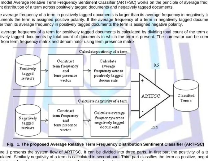
Our model Average Relative Term Frequency Sentiment Classifier (ARTFSC) works on the principle of average frequency count distribution of a term across positively tagged documents and negatively tagged documents.
If the average frequency of a term in positively tagged documents is larger than its average frequency in negatively tagged documents the term is assigned positive polarity. If the average frequency of a term in negatively tagged documents is larger than its average frequency in positively tagged documents the term is assigned negative polarity.
The average frequency of a term for positively tagged documents is calculated by dividing total count of the term across positively tagged documents by total count of documents in which the term is present. The numerator can be computed and from term frequency matrix and denominator using term presence matrix.
Fig. 1. The proposed Average Relative Term Frequency Distribution Sentiment Classifier (ARTFSC) Figure 1 presents the system flow of ARTFSC. It can be divided into three parts. In first part the positivity of a term is calculated. Similarly negativity of a term is calculated in second part. Third part classifies the term as positive, negative or neutral based on its proportion of positivity and negativity calculated in previous steps.
In the first part term presence vector and term frequency vector are constructed in “(6)” and “(7)” for positively tagged documents using “(4)” and “(5)”.
(4)
Where,
TFP=Term Frequency Matrix for Positively tagged documents t = term d = document
TFP[i][j] = cij = count of term i in document j
Where,
TPP = Term Presence Matrix for Positively tagged documents. t = term. d = document.
TPP[i][j] = pij = presence of term i in document j
= 1 if term i is present in document j otherwise 0.
Using the term frequency and presence matrix, frequency of term in positively tagged documents and number of positive documents that contain term t can be computed as follows.
(6)
Where,
Pctd = Frequency of term t in positively tagged documents.
ctj = count of term t in jth document.
(7)
Where,
Pt = Number for positively tagged documents with term t.
ptj = presence of term t document j
In “(8)” average frequency of the terms is calculated by using the vectors in “(6)” and “(7)” of positively tagged documents. This value contributes of the positivity of the terms. This step helps in reducing the impact of spam reviews and noise if any. Even if few biased reviews exist, their frequencies are suppressed (although not eliminated) by denominator of “(8)”.
(8) Where,
Post = Positivity of term t.
Pctd = Frequency of term t in positively tagged documents.
Pt = Number for positively tagged documents with term t.
Similarly in second part the negatively tagged documents are represented as document vectors i.e. in form of term presence vector and term frequency vector. Negativity of the terms is calculated using average frequency of term in negatively tagged documents, vectors, as in “(9)”.
(9) Where,
Negt = Negativity of term t.
Nctd = Frequency of term t in negatively tagged documents.
Nt = Number for negatively tagged documents with term t.
If positivity of a term is larger than negativity of the same term than the term is classified as positive. Conversely, if negativity of a term is larger than positivity of the same term then the term is classified as negative in the third part using “(10)” and “(11)”. A term is classified as neutral if its positivity equals negativity.
(10)
Where,
LDPt = Logarithmic differential Polarity.
Post = Positivity of term t.
1 > 0
Polt= 0 if LDPt = 0 (11)
-1 < 0
Where,
Polt = Polarity of term t.
LDPt = Logarithmic differential Polarity.
If negativity of a term was zero the model would have been affected by divide by zero error. So we added a small value 0.001 to Negt i.e. denominator part. As a result, the term was classified as positive if positivity of term was nonzero and
neutral if positivity of the term was also zero.
Similarly if Post =0 and Negt is not equal to zero then the term should be classified as negative. This is accomplished by
adding a negligible value 0.001 to the numerator.
Stop-words are handled while computing Post and Negt, in “(8)” and “(9)”. If a term frequently occurred in many positive
and negative documents then Post approximately equals Negt. Thus LDPt = log 1 = 0 and Polt would be computed zero
using “(10)” and “(11)”. These are classified as neutral terms.
Our model handles specialized class of stop-words called as senti-stop-words. The terms whose positivity equals negativity are classified as neutral using “(10)” as log 1 equals zero.
There might be Senti stop-words whose positivity and negativity might are not exactly evenly distributed so we varied parameters in experiment 1 to further improve our model. Senti-stop word differs from stop word depending on its distribution across documents of both classes.
IV. EXPERIMENTS CONDUCTED
Pang and Lee’s movie dataset with 1000 positively tagged text documents and 1000 negatively tagged text document were used in all the experiment. These review text files size varied from 1KB to 15 KB. Number of words per document varied from 17 to 2678.
A list of terms that occurred in the documents was prepared. A term is entered only once in this term list. A document vector was constructed for every document. Every ith element in this vector was count of ith term in this document. If a term in term list was not present in the document the count associated with that term was set to zero. These vectors were used to calculate term polarity for the terms in the term list. Polarity was calculated using proposed ARTFSC model as well as Delta TFIDF model described in section 3 and 2 respectively.
A term was classified either as positive or negative or neutral.The terms that occurred in only one document were ignored.A document was classified by our model as positive if total number of positive terms in the document were more than negative terms. Similarly a document was classified as negative if total number of negative terms in the document were more than positive terms. If a document was originally tagged as positive & also classified as positive then it contributed to True Positive in confusion matrix. If a document was originally tagged as negative & also classified as negative then it contributed to True Negative. If a document was originally tagged as positive but classified as negative then it contributed to False Negative. If a document was originally tagged as negative but classified positive then it contributed to False Negative.
A. Experiment 1
Experiment 1 was conducted to determine that a term t should be classified as Senti-stop-word if LDPt equals zero or it
was within a specified range. For this accuracy was computed using, 10 Fold Cross Validation (10 fold CV), varying the range of LDPt between 0 to 1 at step of 0.1 and simultaneously 0 to -1 at step of -0.1.
To calculate accuracy dataset was divided in 10 parts. At every fold this 10% dataset was used for testing and remaining 90% dataset was used for training the classifier. Confusion matrix was constructed as well as accuracy was calculated at every fold and then averaged to form the accuracy of the model.
B. Experiment 2
10 Fold Cross Validation (10 fold CV) technique [4] was used to calculate accuracy of ARTFSC and Delta TFIDF. Dataset was divided in 10 parts. At every fold this 10% dataset was used for testing and remaining 90% for training the classifier. LDPt range was now and for all further experiments was set to -0.6 to 0.6 as determined in experiment 1 for a term to be
classified as neutral. Confusion matrix was constructed as well as accuracy was calculated at every fold and then averaged to form the accuracy of the model at that value of LDPt.
C. Experiment 3
Accuracy was calculated using 10% of the dataset as training set and remaining 90% as the test set. Training dataset was incremented by 10% and remaining was used as test data in further iterations till 90% data was used for training and 10% for testing. Accuracy was calculated at every repetition.
D. Experiment 4
Accuracy was calculated using the entire dataset for training set as well as for testing
V. RESULTS AND DISCUSSION
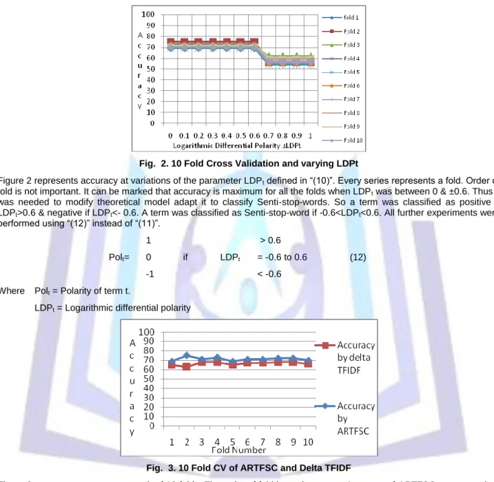
Fig. 2. 10 Fold Cross Validation and varying LDPt
Figure 2 represents accuracy at variations of the parameter LDPt defined in “(10)”. Every series represents a fold. Order of
fold is not important. It can be marked that accuracy is maximum for all the folds when LDPt was between 0 & ±0.6. Thus it
was needed to modify theoretical model adapt it to classify Senti-stop-words. So a term was classified as positive if LDPt>0.6 & negative if LDPt<- 0.6. A term was classified as Senti-stop-word if -0.6<LDPt<0.6. All further experiments were
performed using “(12)” instead of “(11)”.
1 > 0.6
Polt= 0 if LDPt = -0.6 to 0.6 (12)
-1 < -0.6
Where Polt = Polarity of term t.
LDPt = Logarithmic differential polarity
Fig. 3. 10 Fold CV of ARTFSC and Delta TFIDF
Figure 3 represents accuracy at each of 10 folds. The order of fold is not important. Accuracy of ARTFSC was more than Delta TFIDF in all folds. The accuracy at every fold was averaged for comparison. The average accuracy of all folds of ARTFSC was 71.3% and that of Delta TFIDF was 66.5%.
Figure 4 represents accuracy of delta TFIDF and ARTFSC when the training dataset is incremented by 10% for all iteration and remaining data is used for testing. For any good classifier the accuracy should increase when training data is increased. Accuracy of ARTFSC as well as delta TFIDF increases as training data is incremented. Accuracy of ARTFSC was more delta TFIDF overall
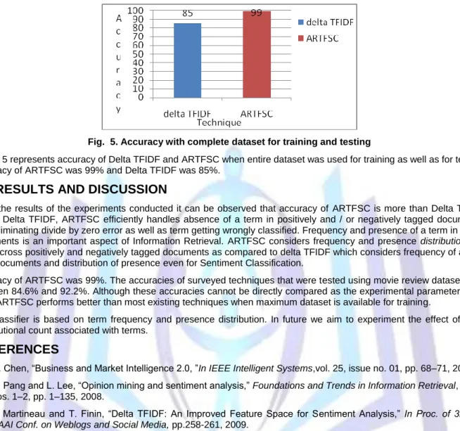
Fig. 5. Accuracy with complete dataset for training and testing
Figure 5 represents accuracy of Delta TFIDF and ARTFSC when entire dataset was used for training as well as for testing. Accuracy of ARTFSC was 99% and Delta TFIDF was 85%.
VI. RESULTS AND DISCUSSION
From the results of the experiments conducted it can be observed that accuracy of ARTFSC is more than Delta TFIDF. Unlike Delta TFIDF, ARTFSC efficiently handles absence of a term in positively and / or negatively tagged documents, thus eliminating divide by zero error as well as term getting wrongly classified. Frequency and presence of a term in all the documents is an important aspect of Information Retrieval. ARTFSC considers frequency and presence distribution of a term across positively and negatively tagged documents as compared to delta TFIDF which considers frequency of a term in all documents and distribution of presence even for Sentiment Classification.
Accuracy of ARTFSC was 99%. The accuracies of surveyed techniques that were tested using movie review dataset were between 84.6% and 92.2%. Although these accuracies cannot be directly compared as the experimental parameters may vary, ARTFSC performs better than most existing techniques when maximum dataset is available for training.
Our classifier is based on term frequency and presence distribution. In future we aim to experiment the effect of other distributional count associated with terms.
REFERENCES
[1] H. Chen, “Business and Market Intelligence 2.0, ”In IEEE Intelligent Systems,vol. 25, issue no. 01, pp. 68–71, 2010. [2] B. Pang and L. Lee, “Opinion mining and sentiment analysis,” Foundations and Trends in Information Retrieval, vol. 2,
nos. 1–2, pp. 1–135, 2008.
[3] J. Martineau and T. Finin, “Delta TFIDF: An Improved Feature Space for Sentiment Analysis,” In Proc. of 3rd Int’l AAAI Conf. on Weblogs and Social Media, pp.258-261, 2009.
[4] L. Lee and B. Pang, “Seeing Stars: Exploiting Class Relationships for Sentiment Categorization with Respect to Rating Scales,” In Proc. of Ann. Meeting Assoc. Computational Linguistics, pp. 115-124, 2005.
[5] E. Cambria, R. Speer, C. Havasi, and Amir Hussain, “SenticNet: A Publicly Available Semantic Resource for Opinion Mining,” In Proceedings of AAAI Conf. on Commonsense Knowledge, pp. 14-18, 2010.
[6] G. Paltoglou and M. Thelwall, “Seeing Stars of Valence and Arousal in Blog Posts,” In IEEE Trans. on Affective Computing, vol. 04, issue no. 01, pp. 116-123, 2013.
[7] C. Lin, Y. He, and R. Everson, “Sentence subjectivity detection with weakly-supervised learning,” In Proc. of 5th Int’l Joint Conf. on Natural Language Processing, pp. 1153–1161, 2011.
[8] E. Cambria, B. Schuller, Y. Xia, and C. Havasi, “New Avenues in Opinion Mining and Sentiment Analysis,” In IEEE Intelligent Systems, vol.28, no.2, pp. 15-21, 2013.
[9] S. Baccianella, A. Esuli, and F. Sebastiani, ” SentiWordNet 3.0: An Enhanced Lexical Resource for Sentiment Analysis and Opinion Mining,” In Proc. of 7th Int’l Conf. on Language Resources and Evaluation, pp 2200-2204, 2010. [10] A. Neviarouskaya, H. Prendinger, and M. Ishizuka, "SentiFul: A Lexicon for Sentiment Analysis," In IEEE Trans. On
Affective Computing, vol. 02, issue no. 01, pp. 22-36, 2011.
[11] Bollegala, D. Weir, and J. Carroll, "Cross-Domain Sentiment Classification using a Sentiment Sensitive Thesaurus," Knowledge and Data Engineering, IEEE Transactions, vol.25, issue no.08, pp. 1, 0
[12] R. Xia and C. Zong, “A POS-based Ensemble Model for Cross-domain Sentiment Classification,” In Proc. of 5th Int’l Joint Conf. on Natural Language Processing, pp. 614–622, 2011.
[13] K. Ghag and K. Shah, "Comparative analysis of the techniques for Sentiment Analysis," In Proc. of Int’l Conf. on Advances in Technology and Engineering, pp. 1-7, 2013.
[14] G. Paltoglou and M. Thelwall, “A study of Information Retrieval weighting schemes for sentiment analysis,” In Proc. of 48th Annual Meeting of the Association for Computational Linguistics, pp. 1386-1395, 2010.
[15] B. Pang, L. Lee, and S. Vaithyanathan, ”Thumbs up? sentiment classification using machine learning techniques,” In Proc. of Conf. on Empirical Methods in Natural Language Processing, pp 79-86, 2002.
[16] T. Mullen and N. Collier, ”Sentiment analysis using support vector machines with diverse information sources,’ In Proc. of Conf. on Empirical Methods in Natural Language Processing,” pp 412–418, 2004.
[17] Charles E. Osgood, George J. Suci, and Percy H. Tannenbaum. The measurement of meaning, 2nd ed.. University of
Illinois Press Urbana, 1967.
[18] P. D. Turney, “Thumbs up or thumbs down? semantic orientation applied to unsupervised classification of reviews,”
In Proc. of the 40th Annual Meeting on Association for Computational Linguistics ACL, pp 417–424, 2002.
[19] O.F. Zaidan, J. Eisner, and C.D. Piatko, “Using Annotator Rationales to Improve Machine Learning for Text Categorization,” In Proc. of Conf. of North American Chapter of the Association for Computational Linguistics, pp 260–267, 2007.
[20] Rudy Prabowo and Mike Thelwall,”Sentiment analysis: A combined approach,” Journal of Informetrics,3(2):143–157,
2009.
[21] Wei-Hao Lin, Theresa Wilson, Janyce Wiebe, and Alexander Hauptmann, ”Which side are you on? identifying perspectives at the document and sentence levels,” In Proceedings of the Conferenceon Natural Language Learning ,2006.
[22] Hugo Liu., “MontyLingua: An end-to-end natural language processor with common sense”. Technical report,MIT, 2004.
[23] R. F. Bruce and J. M. Wiebe, “Recognizing Subjectivity: A Case Study in Manual Tagging,” In Natural Language Engineering, ACM, vol. 05, issue 02, pp 187-205, 1999.
[24] K. Dave, S. Lawrence, and D. M. Pennock, “Mining the Peanut Gallery: Opinion Extraction and Semantic Classification of Product Reviews,” In Proc of the 12th Int’l Conf. on World Wide Web, pp 519 - 528, 2003.
[25] Z. Zhang, "Weighing Stars: Aggregating Online Product Reviews for Intelligent E-commerce Applications," In IEEE Intelligent Systems, vol. 23, issue no.05, pp.42-49, 2008.
[26] J. Wang and A. Dong, “A Comparison of Two Text Representations for Sentiment Analysis,” In Proc. of Int’l Conf. on Computer Application and System Modeling, pp V11-35–V11-39, 2010.
[27] Ghose and P. G. Ipeirotis, "Estimating the Helpfulness and Economic Impact of Product Reviews: Mining Text and Reviewer Characteristics," In Knowledge and Data Engineering, IEEE Transactions, vol.23, issue no.10, pp. 1498-1512, 2011.
[28] G. Li and F. Liu, “A Clustering-Based Approach on Sentiment Analysis,” In Proc. of Int’l Conf. on Intelligent Systems and Knowledge Engineering, pp 331-337, 2011.
[29] X. Yu, Y. Liu, X. Huang, and A. An, "Mining Online Reviews for Predicting Sales Performance: A Case Study in the Movie Domain," In Knowledge and Data Engineering, IEEE Transactions, vol.24, issue no.04, pp. 720-734, 2012. [30] Lin, Y. He, R. Everson, and S. Ruger, "Weakly Supervised Joint Sentiment-Topic Detection from Text," In Knowledge
and Data Engineering, IEEE Transactions, vol.24,issue no.06, pp. 1134-1145, 2012.
[31] A. Kumar and N. Ahmad, “ComEx Miner: Expert Mining in Virtual Communities”, In International Journal of Advanced
Computer Science and Applications, vol.03, issue no 06, pp 54-65, 2012.
[32] A. Hamouda and F. El-taher, "Sentiment Analyzer for Arabic Comments System," International Journal of Advanced Computer Science and Applications, vol. 04, issue no.03, pp 99-103, 2013
[33] C. Hung and H. Lin, "Using Objective Words in SentiWordNet to Improve Word-of-Mouth Sentiment Classification," In IEEE Intelligent Systems, vol.28, no.2, pp. 47-54, 2013.
[34] G. Salton and M. McGill, “Introduction to modern Information Retrieval,” McGraw-Hill, pp. 105-107 & 205,1983. [35] J. Han and M. Kamber, “Data Mining Concepts and Techniques,” Morgan Kaufmann Publishers, 02nd edition, pp.