University of Kentucky University of Kentucky
UKnowledge
UKnowledge
Theses and Dissertations--Computer Science Computer Science 2019
Rule Mining and Sequential Pattern Based Predictive Modeling
Rule Mining and Sequential Pattern Based Predictive Modeling
with EMR Data
with EMR Data
Orhan AbarUniversity of Kentucky, [email protected]
Digital Object Identifier: https://doi.org/10.13023/etd.2019.330
Right click to open a feedback form in a new tab to let us know how this document benefits you. Right click to open a feedback form in a new tab to let us know how this document benefits you. Recommended Citation
Recommended Citation
Abar, Orhan, "Rule Mining and Sequential Pattern Based Predictive Modeling with EMR Data" (2019). Theses and Dissertations--Computer Science. 85.
https://uknowledge.uky.edu/cs_etds/85
This Doctoral Dissertation is brought to you for free and open access by the Computer Science at UKnowledge. It has been accepted for inclusion in Theses and Dissertations--Computer Science by an authorized administrator of UKnowledge. For more information, please contact [email protected].
STUDENT AGREEMENT: STUDENT AGREEMENT:
I represent that my thesis or dissertation and abstract are my original work. Proper attribution has been given to all outside sources. I understand that I am solely responsible for obtaining any needed copyright permissions. I have obtained needed written permission statement(s) from the owner(s) of each third-party copyrighted matter to be included in my work, allowing electronic distribution (if such use is not permitted by the fair use doctrine) which will be submitted to UKnowledge as Additional File.
I hereby grant to The University of Kentucky and its agents the irrevocable, non-exclusive, and royalty-free license to archive and make accessible my work in whole or in part in all forms of media, now or hereafter known. I agree that the document mentioned above may be made available immediately for worldwide access unless an embargo applies.
I retain all other ownership rights to the copyright of my work. I also retain the right to use in future works (such as articles or books) all or part of my work. I understand that I am free to register the copyright to my work.
REVIEW, APPROVAL AND ACCEPTANCE REVIEW, APPROVAL AND ACCEPTANCE
The document mentioned above has been reviewed and accepted by the student’s advisor, on behalf of the advisory committee, and by the Director of Graduate Studies (DGS), on behalf of the program; we verify that this is the final, approved version of the student’s thesis including all changes required by the advisory committee. The undersigned agree to abide by the statements above.
Orhan Abar, Student Dr. Ramakanth Kavuluru, Major Professor Dr. Mirosław Truszczyński, Director of Graduate Studies
Rule Mining and Sequential Pattern Based Predictive Modeling with EMR Data
DISSERTATION
A dissertation submitted in partial fulfillment of the requirements for the degree of Doctor of Philosophy in the College of Engineering at the
University of Kentucky By
Orhan Abar Lexington, Kentucky
Director: Dr. Ramakanth Kavuluru, Associate Professor of Biomedical Informatics Co-Director: Dr. Jinze Liu, Associate Professor of Computer Science
Lexington, Kentucky 2019
ABSTRACT OF DISSERTATION
Rule Mining and Sequential Pattern Based Predictive Modeling with EMR Data Electronic medical record (EMR) data is collected on a daily basis at hospitals and other healthcare facilities to track patients’ health situations including conditions, treatments (medications, procedures), diagnostics (labs) and associated healthcare operations. Besides being useful for individual patient care and hospital operations (e.g., billing, triaging), EMRs can also be exploited for secondary data analyses to glean discriminative patterns that hold across patient cohorts for different pheno-types. These patterns in turn can yield high level insights into disease progression with interventional potential. In this dissertation, using a large scale realistic EMR dataset of over one million patients visiting University of Kentucky healthcare facili-ties, we explore data mining and machine learning methods for association rule (AR) mining and predictive modeling with mood and anxiety disorders as use-cases. Our first work involves analysis of existing quantitative measures of rule interestingness to assess how they align with a practicing psychiatrist’s sense of novelty/surprise corre-sponding to ARs identified from EMRs. Our second effort involves mining causal ARs with depression and anxiety disorders as target conditions through matching methods accounting for computationally identified confounding attributes. Our final effort in-volves efficient implementation (via GPUs) and application of contrast pattern mining to predictive modeling for mental conditions using various representational methods and recurrent neural networks. Overall, we demonstrate the effectiveness of rule min-ing methods in secondary analyses of EMR data for identifymin-ing causal associations and building predictive models for diseases.
KEYWORDS: NLP, Machine Learning, Deep Learning, Association Rule Mining, Contrast Sequential Rule Mining, Causal Association
Author’s signature: Orhan Abar
Rule Mining and Sequential Pattern Based Predictive Modeling with EMR Data
By Orhan Abar
Director of Dissertation: Ramakanth Kavuluru
Co-Director of Dissertation: Jinze Liu
Director of Graduate Studies: Mirosław Truszczyński
To my parents Yeter and Mehmet, my wife Tugba and daughter Erva, and my brothers and sisters.
ACKNOWLEDGMENTS
While completing this dissertation, I have received great deal of support and assis-tance. First of all, I would like to express my deepest appreciation to my adviser Dr. Ramakanth Kavuluru for his invaluable contribution, suggestions, experience, and patience. I would like to extend my sincere thanks to my committee members: Dr. Richard Charnigo, Dr. Jinze Liu, and Dr. Dakshnamoorthy Manivannan for par-ticipating in my committee.
I gratefully acknowledge the help of Mehmet Bakal. I also had great pleasure of working with Dr. Gregory Heileman for my final year of study. I would like to thank the ministry of national education of Turkey for their full financial support. Finally, I would like to thank my family for all their relentless support during my studies.
TABLE OF CONTENTS
Acknowledgments . . . iii
Table of Contents . . . iv
List of Tables . . . vi
List of Figures . . . vii
Chapter 1 Introduction . . . 1
1.1 What is an EMR? . . . 1
1.2 Applications of EMRs . . . 2
1.3 Overview of this Dissertation . . . 3
Chapter 2 Related Work and Background . . . 7
2.1 Healthcare Cost and Utilization Project . . . 7
2.2 Association Rule Mining . . . 8
2.3 Term Frequency-Inverse Document Frequency . . . 10
2.4 Odds Ratio . . . 11
2.5 Inter-Rater Reliability Scores . . . 12
2.6 Sequential Contrast Pattern Mining . . . 14
2.7 Recurrent Neural Network (RNN) . . . 15
2.7.1 Vanilla Long Short Term Memory (V-LSTM) . . . 16
2.7.2 Gated Recurrent Unit (GRU) . . . 17
Chapter 3 On Interestingness Measures for Mining Statistically Significant and Novel Clinical Associations from EMRs . . . 19
3.1 Introduction . . . 19
3.1.1 Notions of Statistical Strength, Novelty, & Interestingness . . 20
3.1.2 Our Contributions . . . 20
3.2 AR Mining from Visits Data . . . 21
3.2.1 Clinical Dataset Used . . . 22
3.2.2 Generating Association Rules . . . 23
3.3 Assessing Interestingness Measures for Association Rule (AR) Ranking 24 3.3.1 Additional Interestingness Measures . . . 24
3.3.2 Domain Expert Novelty Assessments . . . 25
3.3.3 Comparison of Interestingness Measures . . . 27
3.4 Quantitative & Qualitative Analysis of Novel Rules . . . 29
3.5 Concluding Remarks . . . 31
Chapter 4 Toward Causal Association Rule Mining . . . 33
4.2 Clinical Dataset Used . . . 36
4.3 CAR Mining From Patient Data . . . 38
4.3.1 Generating Confounders . . . 38
4.3.2 Causal Association Rules . . . 39
4.4 Experiments and Results (Quantitative & Qualitative Analysis of CARs) 44 4.4.1 Causality Scores . . . 45
4.4.2 Domain Expert Assigned Plausibility Scores . . . 46
4.4.3 Comparison of Scores . . . 48
4.5 Conclusion . . . 50
Chapter 5 Predictive Modeling through Sequential Patterns and Recurrent Neural Network (RNNs) . . . 52
5.1 Related works . . . 53
5.2 The EMR Database and Cohort Selection . . . 56
5.3 Methods . . . 58
5.3.1 Support Counting on GPUs and Parallel Reduction . . . 58
5.3.2 Creating Sequential Pattern Based Database . . . 59
5.3.3 Input Representations . . . 61
5.3.4 RETAIN Model . . . 64
5.3.5 DeepCare Model . . . 65
5.3.6 Two Level Hierarchical LSTM Model . . . 67
5.3.7 Combining Our Model with V-LSTM . . . 68
5.4 Results and Discussion . . . 69
5.4.1 Experimental Setup . . . 69
5.4.2 Models . . . 70
5.4.3 Comparing the Results of Models . . . 71
5.5 Conclusion . . . 76
Chapter 6 Conclusion . . . 78
Abbreviations . . . 80
Bibliography . . . 83
LIST OF TABLES
2.1 List of International Classification of Diseases, Clinical Modification, 9th
revision (ICD-9-CM) codes related to depressive disorders . . . 8
2.2 List of ICD-9-CM codes related to anxiety disorders . . . 9
2.3 2 × 2 Contingency Table for Rule E ⇒Y . . . 11
2.4 2×2 Contingency table for the assessment of IRR . . . 12
2.5 The agreement level of IRR measures . . . 14
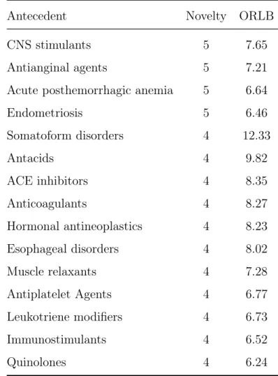
3.1 Antecedents with novelty ≥4 and ORLB ≥5 . . . 30
4.1 List of ICD-9-CM codes related to targeted disorders . . . 38
4.2 2×2 Contingency table for a ruleE ⇒Y on FD . . . 42
4.3 The list of criteria to create FD . . . 46
4.4 Statistics for CARs . . . 46
4.5 Scores assigned by raters for CARs . . . 47
4.6 IRR scores for raters . . . 48
4.7 Scores assigned by raters for CARs . . . 48
4.8 Rater graded scores . . . 49
5.1 List of variables and possible values to generate database variations.N/S used as value when there is no limitation specified. . . 56
5.2 Classes for BMI and age of a patient . . . 57
5.3 Positive and negative class sizes for each cohort . . . 58
5.4 Sequence ordering criteria . . . 60
5.5 The EMR database statistics used for predictive modeling for depressive disorders . . . 70
5.6 Comparison of the results of models with different input representations: the concatenated MPEmb version versus original version. Mean is taken over the differences from model performances on all 32 cohorts. . . 72
5.7 Comparison of results for original V-LSTM model without demographics with the V-LSTM model using ConCat Embedding across all 32 cohorts 73 5.8 Comparison of results for original Doctor AI model with Doctor AI model using ConCat embedding across all 32 cohorts . . . 74
5.9 Comparison of results for original RETAIN model with RETAIN model using ConCat embedding across all 32 cohorts . . . 75
5.10 Comparison of results for original DeepCare model with DeepCare model using ConCat embedding across all 32 cohorts . . . 76
5.11 Comparing results using washout period: 6 months, max-CVG: 12 months, prediction horizon window: 12 months, and min patient visit size: 30, with our hierarchical and the combined models. . . 77
LIST OF FIGURES
2.1 Number of ICD-9-CM codes for each CSS classes . . . 7
2.2 Sequential Contrast Pattern Mining Scheme . . . 15
2.3 LSTM structure . . . 16
2.4 GRU structure . . . 18
3.1 Interestingness measure profiles with novelty-statistical strength trade-offs 26 4.1 Number of visits and patient to the UKY hospital and affiliated clinics for each year . . . 37
4.2 Forest plot of top 10 exposures for depressive disorders . . . 49
4.3 Forest plot of top 10 exposures for anxiety disorders . . . 50
4.4 Average score for related percentage for anxiety disorders and depressive disorders . . . 51
5.1 Patient visit history . . . 56
5.2 Unfolding parallel reduction steps . . . 59
5.3 Sequence of sequential patterns encapsulating a patient’s visit history . . 60
5.4 Example ordered TSCP based on patterns in Figure 5.3 . . . 61
5.5 Transformation to the multi-hot representation . . . 61
5.6 EMR embedding layer and mean pooling . . . 62
5.7 Concatenate embedding layer with mean pooling for input representation 63 5.8 The RETAIN longitudinal EMR modeling architecture . . . 64
5.9 C-LSTM structure used in DeepCare model . . . 66
5.10 2-level hierarchical SCP based neural architecture for predictive modeling through longitudinal EMRs . . . 68
Chapter 1 Introduction
Increased digitization of data from various facets of our daily lives (including shop-ping runs, fitness activities, hospital visits, and social media interactions) necessitates new methodological advances in collecting, integrating, and mining extremely large datasets. Many data mining algorithms have been proposed during the past three decades in order to extract useful information from these large datasets. Such algo-rithms are currently used in fields such as chemistry, finance, e-commerce, biomedicine, and healthcare. In particular, the healthcare field has seen a major surge of appli-cations of data mining mostly due to the deluge of digital data captured through electronic medical records (EMRs). However, this area poses significant challenges due to the high dimensionality (tens of thousands of variables), inherent errors, pri-vacy concerns, and missing values. Our main goals are to leverage this EMR data to identify interesting associations between different biomedical variables of interest (potentially leading to new insights and hypotheses) and to build predictive models to identify high risk patients for chronic conditions. Next, we discuss the various patient attributes available in EMRs considered for this dissertation.
1.1 What is an EMR?
An EMR is a digital record that gets generated for each visit a patient makes to a healthcare facility (e.g., hospital, emergency room, diagnostic lab, private clinic). As such, each patient, as they go through a healthcare system, generates a trail (specif-ically, a temporally ordered sequence) of EMRs, one per visit. An EMR contains patient demographic information including the name of the patient, their gender, and age. Basic variables such as height and weight (hence body mass index (BMI)) and smoking status may also be recorded. More importantly, depending on the visit, an EMR may also have the following elements.
• At least one diagnosis code assigned from the standard terminology – inter-national classification of diseases: clinical-modification standards (ICD-9/10-CM). These codes represent different conditions the patient has been diagnosed with during the visit.
• Depending on the nature of the visit, EMRs may also contain procedure codes from the current procedure terminology (CPT) standard for any procedures
performed (e.g., surgery) during the visit.
• If diagnostic lab tests (e.g., lipid panel) are done, values measured for differ-ent biomarkers (e.g., cholesterol) may be recorded typically using the logical observation identifiers, names, and codes (LOINC) terminology.
• Any medications administered during the visit or prescribed for subsequent usage will also be recorded via a standard terminology such as the national drug code (NDC).
• Besides these structured variables, free text is often included (especially for in-patients) in the form of admission notes, progress notes, pathology/radiology reports, and discharge summaries. Intuitively, the free text notes are expected to contain case-specific elaborate details that are not captured in any of the structured sources covered earlier (e.g., observed side affects, social variables including employment/marital status).
1.2 Applications of EMRs
As the digital encapsulations of a patient’s health related events, EMRs are essential in improving the operational side of delivering patient care. EMRs are instrumental in maintaining continuity of care as patients go through different providers within a healthcare system. For instance, they can be crucial in ensuring patients obtain prescriptions that do not interfere with their existing medications. On the fiscal side, EMRs (esp. the structured codes) are also critical in determining what the patient or their insurance firm ought to be charged for the services the healthcare facility or the physician has provided.
Due to recent rapid adoption of EMRs among many facilities and better linking of records between different clinics that belong to larger systems, massive EMR datasets are being curated for millions of patients. If the healthcare system covers a reason-ably sized neighborhood, one could argue that, the chronological aggregation of a patient’s EMRs constitutes their longitudinal EMR (LEMR). Although there may be occasional visits to non-local clinics, given how insurance policies are tailored to mini-mize co-pay and other out-of-pocket expenses for in-network visits, patients are likely to limit most of their visits to a single healthcare system. The only exception to this assumption is when patients move permanently to a different location, which is easy to spot in their record based on the duration from their last visit to an in-network
through the healthcare system. Both visit-level EMRs and patient-level LEMRs are hence becoming goldmines for deriving insights across populations (as opposed to their main purpose: individual patient care). With the evolution of data science as a discipline and the rise of precision medicine initiatives for targeted therapies, (L)EMRs are being repurposed for disease phenotype discovery, predictive modeling, computational drug discovery and repositioning, cohort selection, and causal asso-ciation mining. This secondary data analyses of EMR data for deriving insights at the patient population level is the main focus of this thesis. Next, we present a brief overview of this dissertation.
1.3 Overview of this Dissertation
This dissertation focuses on (1). assessing the potential of data mining approaches for extracting statistically significant and causal associations from EMRs; (2). predicting chronic conditions from LEMRs using recent advances in contrast pattern mining and deep neural networks. Although current approaches have been shown to obtain promising results, developing new approaches and/or cleverly configuring existing ones may create more predictive power and improve the quality of the outcomes as outlined in the following chronological introduction to the main ideas behind this dissertation.
• Interestingness measures for association rule mining (ARM): Over the past two decades, ARM has received significant attention from both the data mining and machine learning communities. While data mining researchers focus on designing efficient algorithms to mine rules from large datasets, the learning community has explored applications of rule mining to classification. A major problem with rule mining algorithms is the explosion of rules even for moderate sized datasets making it extremely difficult for end users to identify both statis-tically significant and potentially novel rules that could lead to interesting new insights and hypotheses. Researchers have proposed many domain independent interestingness measures using which, one can rank the rules and potentially glean useful rules from the top ranked ones. However, these measures have not been fully explored for rule mining in clinical datasets owing to the relatively large sizes of the datasets often encountered in healthcare. Additionally, limited access to domain experts creates another obstacle for the review/analysis.
In the first part of this dissertation, using an EMR dataset of 3.25 million visits to UKHealthcare clinics, we studied the trade-off between rule novelty and
statisti-cal significance using dozens of interestingness measures proposed in the literature and also a few additional measures we devised for this study. The rules we studied are of the form E ⇒ Y where E (antecedent) and Y (consequent) are item sets formed from unique clinical variables: diagnoses, medications, procedures, and labs. Typically (including in our analysis), Y is a singleton and in biomedicine it is set to a medical/mental condition of interest. Here, we limited our analysis to only medications and diagnoses in our initial work and our consequent of choice is depressive disorders. The assessment of novelty of rules is conducted by a prac-ticing psychiatrist (Dr. Rayapati) of UKHealthcare. Our results not only surface new interesting associations for depressive disorders but also indicate classes of interestingness measures that weight rule novelty and statistical strength in con-trasting ways, offering new insights for end users in identifying interesting rules. The details of the methods used and results of this work are published in ACM BCB 2016 (Abar et al., 2016) and are presented in Chapter 3.
• Toward causal association rule (CAR) mining: Although association rules of the form E ⇒ Y are interesting for further exploration, they may only indi-cate correlations that may be spurious. In fields such as biomedicine, it is more meaningful to identify causal association rules, where the antecedent E can be thought of as an event (e.g., taking a medication) that maybe causing the con-sequent Y (e.g., a condition, potentially as a side effect). Causal inference in biomedicine is a highly nuanced subject but most definitions of causality have a set of shared guidelines formulated by English epidemiologist Austin Bradford Hill in 1965. An obvious guideline is temporal precedence of E with respect of Y. So mining at patient-level LEMRs (the chronological EMR history) is a prerequisite. Additionally, the association must hold after accounting for potential confounding attributes, variables that may influence E and Y leading to a spurious correlation between the pair. Other guidelines involve establishing/identifying the existence of an actual plausible biomedical mechanism through which the causal association manifests and evidence through experiments (e.g., randomized controlled trials). Given our sandbox is the retrospective observational data in EMRs, we cannot account for all requirements needed for causality. But, we can account for con-founders and ensure temporal precedence. With circumspection, we hence qualify our effort as moving “toward” CAR mining. Intuitively, however, CARs form a smaller and manageable high confidence hypothesis space compared with the full set of associations curated from EMRs.
A major challenge for CAR mining even in the retrospective setup is that all confounders are not known ahead of time besides the common ones such as gender, age, and race. Furthermore, approaches that rely on learning Bayesian networks (BNs) automatically from data do not scale to datasets with large variable spaces such as those encountered here. CAR mining is a more practical alternative for observational studies but has not been fully explored in current literature. In this dissertation, using an LEMR dataset of over 900,000 patient records with more than four million patient visits to the UKY medical center and affiliated clinics, we studied the causal effects involving diagnoses and medications, and patient demographics on two mental conditions: depressive disorders and anxiety disorders. The process of generating CARs starts with computational confounder detection. Next, using these confounders, we generate the so called “fair” datasets (FDs) that consist of matched LEMR pairs to calculate the strength of possible CAs. Then, rules with 95% CI-based odds-ratio lower bounds (ORLBs) greater than one, as calculated from the FDs, are selected as CARs. Finally, we compare these ORLB based causality rankings against expert judgments which are obtained from two practicing psychiatrists to assess the utility of our method. We identify interesting CARs and also find that the causality ratings produced by our method align with those assigned by the domain experts. Full details of this effort and corresponding findings are presented in Chapter 4.
• Predictive modeling with contrast patterns and neural networks: One in four Americans and three in four Americans aged 65 and older suffer from multiple chronic conditions leading to 71% of total healthcare spending in the U.S. Both in terms of sheer suffering and high out-of-pocket expenses, patients with multiple chronic conditions form a subgroup that are deservedly getting attention from the research and health services communities. Once diagnosed with such conditions, patients are usually on corresponding medications for the rest of their lives. Also, multiple chronic comorbidities greatly compromise immunity and can make people highly susceptible to acute infections that can rapidly lead to multiple organ failure. Thus, being able to predict such conditions well before they manifest fully can be of immense preventative and interventional value, which is clearly something all stakeholders — patients, doctors, healthcare facilities, insurance providers, and health policymakers — can get behind.
Because LEMRs represent patient trajectories through the healthcare system, we can use supervised machine learning methods that take as input a prefix of a
pa-tient’s LEMR and predict their future conditions. This can be further simplified, if we formulate it as estimating the probability of first diagnosis of a particular chronic condition in the future, predicted at different time horizons. In this dis-sertation, this is the line of work pursued for depressive disorders as the target condition group using different neural-network based representations of LEMRs. Unlike prior efforts that only employ recurrent neural network (RNN) variants, we also employ sequential contrast patterns (SCPs) derived from LEMRs and use RNN based sequence compositions on top of SCPs. By carefully varying washout periods, future time horizons, maximum inter-visit gaps, and minimum numbers of visits, we first examine the performance of existing LEMR based predictive mod-eling methods for different variants of LEMR input encoding. Next, we choose a particular cohort of patients (diagnosed with depressive disorders) with a washout period of six months, a one year maximum inter-visit gap, and with at least 30 vis-its made to UKHealthCare facilities. Using this data, we predict the first diagnosis of depressive disorders with a one year time horizon. We apply our novel model-ing approach that hierarchically composes SCPs and SCP sequences usmodel-ing RNNs. Our results show that a hybrid model that combines a conventional RNN with our SCP-based RNN produces the best predictive performance. These models, their variants, and results are presented in Chapter 5.
Chapter 2 Related Work and Background
In this chapter, we will describe background concepts that are essential to the rest of the dissertation.
2.1 Healthcare Cost and Utilization Project
The HCUP (Healthcare Cost and Utilization Project, n.d.) aims to generate health-care related datasets and software tools to build national data resources. Diagnosis and procedure classification via HCUP is carried out through its clinical classification software (CCS), which is used to group various diagnosis codes in this dissertation. HCUP has been created by the Agency for Healthcare Research and Quality (AHRQ), a federal organization that oversees and guides health services and care delivery as-pects at the national level. The purpose of developing CSS is to generate clinically
0 50 100 150 200 250 300 0 200 400 600 800 1,000 1,200 1,400 1,600 CSS class Num b er of ICD-9-CM co de
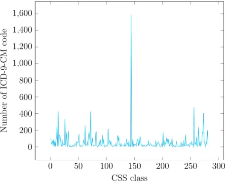
Figure 2.1: Number of ICD-9-CM codes for each CSS classes
meaningful classification of ICD and CPT codes. Instead of using a single code, using a group of codes related to same diagnosis or procedure is more beneficial in statistical studies to obtain high level estimates as opposed to estimates for all suble variants created originally for billing purposes. For example, ICD-9-CM consists of more than
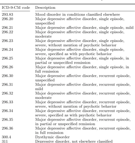
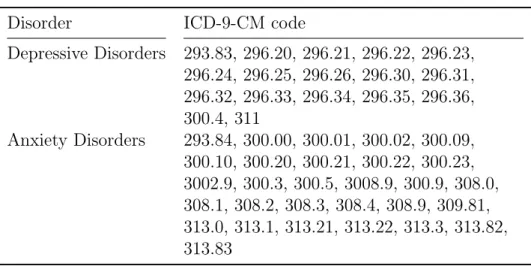
14,000 diagnosis codes and these codes can be classified into 282 different classes us-ing CSS’ classification system. Figure 2.1 shows the number of ICD-9-CM codes in each CSS classe. While some classes are small, some have a large number of ICD-9-CM codes. For instance, class 144 (multi-level CSS category 18) “Residual codes; unclassified; all E codes” has 1589 different ICD-9-CM codes which is the class with highest number of codes while class 55 (multi-level CSS category 5.3.2) “Oppositional defiant disorder” has exactly one code. Tables 2.1 and 2.2 presents ICD-9-CM codes and descriptions related to depressive disorders and anxiety disorders respectively.
Table 2.1: List of ICD-9-CM codes related to depressive disorders ICD-9-CM code Description
293.83 Mood disorder in conditions classified elsewhere 296.20 Major depressive affective disorder, single episode,
unspecified
296.21 Major depressive affective disorder, single episode, mild 296.22 Major depressive affective disorder, single episode,
moderate
296.23 Major depressive affective disorder, single episode, severe, without mention of psychotic behavior 296.24 Major depressive affective disorder, single episode,
severe, specified as with psychotic behavior
296.25 Major depressive affective disorder, single episode, in partial or unspecified remission
296.26 Major depressive affective disorder, single episode, in full remission
296.30 Major depressive affective disorder, recurrent episode, unspecified
296.31 Major depressive affective disorder, recurrent episode, mild
296.32 Major depressive affective disorder, recurrent episode, moderate
296.33 Major depressive affective disorder, recurrent episode, severe, without mention of psychotic behavior 296.34 Major depressive affective disorder, recurrent episode,
severe, specified as with psychotic behavior
296.35 Major depressive affective disorder, recurrent episode, in partial or unspecified remission
296.36 Major depressive affective disorder, recurrent episode, in full remission
300.4 Dysthymic disorder
311 Depressive disorder, not elsewhere classified
2.2 Association Rule Mining
LetI be the union of all medications and diagnoses and any other biomedical variables that are of interest for each patient. For our purposes, a set E ={i1, . . . , ik} ⊆ I is
called a clinicalitem set withk items and a patient visit transaction T = (pid, vid, I)
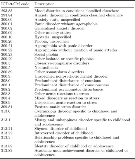
Table 2.2: List of ICD-9-CM codes related to anxiety disorders ICD-9-CM code Description
293.83 Mood disorder in conditions classified elsewhere 293.84 Anxiety disorder in conditions classified elsewhere 300.00 Anxiety state, unspecified
300.01 Panic disorder without agoraphobia 300.02 Generalized anxiety disorder 300.09 Other anxiety states 300.10 Hysteria, unspecified 300.20 Phobia, unspecified
300.21 Agoraphobia with panic disorder
300.22 Agoraphobia without mention of panic attacks 300.23 Social phobia
300.29 Other isolated or specific phobias 300.3 Obsessive-compulsive disorders 300.5 Neurasthenia
300.89 Other somatoform disorders
300.9 Unspecified nonpsychotic mental disorder 308.0 Predominant disturbance of emotions 308.1 Predominant disturbance of consciousness 308.2 Predominant psychomotor disturbance 308.3 Other acute reactions to stress 308.4 Mixed disorders as reaction to stress 308.9 Unspecified acute reaction to stress 309.81 Posttraumatic stress disorder
313.0 Overanxious disorder specific to childhood and adolescence
313.1 Misery and unhappiness disorder specific to childhood and adolescence
313.21 Shyness disorder of childhood 313.22 Introverted disorder of childhood
313.3 Relationship problems specific to childhood and adolescence
313.82 Identity disorder of childhood or adolescence 313.83 Academic underachievement disorder of childhood or
adolescence
a given database is denoted as the visit database V. A visit transaction (pid, vid, I)
is said to support an item set E if E ⊆I and the support of E in the databaseV is defined as:
support(E,V) = |{vid: (pid, vid, I)∈ V, E ⊆I}|. (2.1) An item set is deemedfrequent if its support is greater than a given minimum support
σ. Thus, the set of frequent item sets with respect to σ is defined as:
F(V, σ) ={E :support(E,V)≥σ}. (2.2)
Next, an Association Rule (AR) is a rule of the form E ⇒ Y where E and Y are item sets andE∩Y =∅. The confidence of an association rule E ⇒Y denoted by
conf(E ⇒Y,V) = support(E∪Y)
models the probabilityP(Y|E)and establishes the association of the consequent item setY with the antecedent item setE. Beside minimum support for item sets, we can establish a minimum confidence γ for ARs and define a stronger notion of frequent and confident ARs over a visit databaseV as the set
R(V, σ, γ) = {E ⇒Y :E∪Y ∈ F(V, σ), conf(E ⇒Y)≥γ}, (2.4) which consists of confidence thresholded ARs obtained from frequent item sets.
2.3 Term Frequency-Inverse Document Frequency
Term Frequency - Inverse Document Frequency (TF-IDF) (Robertson, 2004) is a commonly used statistical method in information retrieval. This is simple yet powerful formula measures the relationship of the term with a given document in corpus. Higher TF-IDF value indicates that the term have strong relationship with a given document. TF-IDF consist of two numerical values; Term Frequency (TF) and Inverse document frequency (IDF). TF-IDF value of a term for a given document in a corpus is defined as:
T F −IDF(ti, d,C) = T F(ti, d)×IDF(ti,C) (2.5)
First value, TF, calculated as the number of occurrence of a term in a specific docu-ment in other word frequency of the term. TF value is defined as:
T F(ti, d) =f requency(ti, d) (2.6)
Second value, IDF, is used to distinguish more meaningful words in a document. For instance, articles “the”, “a”, and “an” tend to occur in every text document in the corpus even if it has no meaning by itself. The idea is to give higher values to the word occurs in less documents to increase the importance of the document specific words. The basic and most commonly used formula to calculate IDF for a document collection and a term, is defined as
IDF(ti,C) = log N ni (2.7)
In order to calculate IDF of the term ti in a corpus C, in equation (2.7), ni is the
number of documents contains the term, ti, where {ti : d ∈ C, ti ∈ d} and d
2.4 Odds Ratio
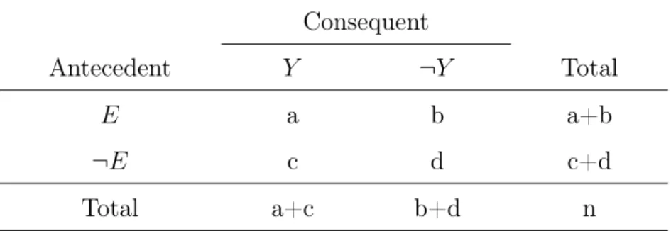
Odds Ratio (OR) (Morris and Gardner, 1988) is a commonly used statistical mea-surement to calculate the association of the exposure, a disease or medication, and the outcome, a medical condition. Table 2.3 shows a 2×2 contingency table for an AR. In this table, calculating OR gives the association between antecedent and conse-quent where antecedent means a exposed disease or medication as well as conseconse-quent corresponds to an another medical condition to relate. OR of an AR is calculated as
OR(E ⇒Y) = a×d
b×c, (2.8)
where E ⇒ Y is an AR and a, b, c, and d are the values appear in the Table 2.3. An association between the exposure and the outcome is decided according to the OR value calculated. There are three different possible values of the calculation. If
OR= 1, there is no association between the exposure and the outcome because odds of the outcome for the exposure is equal to odds of the outcome for not exposure. If OR > 1, there is a positive association between the exposure and the outcome as well as the odds of the outcome significantly increases when it is exposed to the antecedent. If OR <1, the odds of the outcome is lower for the exposure.
Consequent
Antecedent Y ¬Y Total
E a b a+b
¬E c d c+d
Total a+c b+d n
Table 2.3: 2 ×2 Contingency Table for Rule E⇒Y
Calculating the OR is not always enough to ascertain the association between the antecedent and the consequent. Therefore, we will also calculate the Confidence Interval (CI) to estimate the precision of OR. In order to calculate CI, we will first calculate Standard Error (SE). The formula to calculate SE for ln(OR)is defined as:
SE(ln(OR)) = r 1 a + 1 b + 1 c + 1 d. (2.9)
as: ORLB(E ⇒Y) = e ln(OR)−1.96×SE(ln(OR)) (2.10) and ORU B(E ⇒Y) = e ln(OR) + 1.96×SE(ln(OR)) (2.11) Equation 2.10 and Equation 2.11 show how to apply SE value to OR after calculating SE shown in Equation 2.9. These formulas, ORLB and ORUB, are calculated for the 95% confident interval. One of the advantages of using SE other than strengthening association is to avoid misjudgment caused by very small a, b, c, or d values.
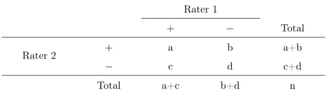
2.5 Inter-Rater Reliability Scores
Many studies in biomedical domain involve observational rating scores from multiple people to demonstrate robustness of the annotation and the corresponding computa-tional methodology. When there is more than one rater, the assessment of inter-rater reliability (IRR) is required to measure the degree of consistency among raters (Hall-gren, 2012). IRR score shows the degree of homogeneity or consensus between the ratings given by the raters. There are a number of statistical measures to assess IRR in the medical domain including Cohen’s Kappa (McHugh, 2012; Cohen, 1960; Cohen, 1968), Spearman’s Rho (Mukaka, 2012), and Gwet’s AC1Wongpakaran et al., 2013; Gwet, 2014. We will start by creating a 2×2 contingency table as shown in Table 2.4 to explain how each measure is calculated.
Table 2.4: 2×2 Contingency table for the assessment of IRR
Rater 1
+ − Total
Rater 2 + a b a+b
− c d c+d
Total a+c b+d n
One of the most frequently used statistics to assess IRR is Cohen’s Kappa also called kappa statistic first introduced in (Cohen, 1960). Cohen’s Kappa symbolized
byκ and ranges between -1 and +1. κ value is calculated as: κ= P(a)−P(e) 1−P(e) (2.12) where P(a) = a+d n , (2.13) and P(e) = (a+c)x(a+b) n + (b+d)x(c+d) n n (2.14)
Another measure to assess IRR, which is frequently used in biomedical domain is the Spearman’s Rho (Spearman, 1904) symbolized by ρ orrs. The value of ρ ranges
from -1 to +1. In order to calculate ρ, first we rank each ratings separately from lowest to highest. Then, for each data pair rank differences are calculated as di.
Finally, ρ is calculated as:
ρ= 1− 6 n P i=1 d2 i n3−n (2.15)
Gwet’s AC1 is also used for the assessment of IRR in biomedical data and was first introduced in (Gwet et al., 2002). As with Cohen’s kappa, Gwet’s AC1 uses probabilistic measurements to calculate IRR score which ranges between -1 and +1. This score is introduced to overcome some issues with κ which can produce different IRR values for same percent of agreement level. Additionally, κ is hard to interpret and unstable. Gwet’s AC1 score is calculated as:
Gwet0s AC1 = P(a)−P(γ)
1−P(γ) (2.16)
where P(a) is calculated as in Equation 2.13 andP(γ) is calculated as:
P(γ) = 2q(1−q) (2.17) with
q = (a+c) + (a+b)
2n . (2.18)
According to the value calculated by an IRR measurement, 1 means that the degree of consistency among the raters is perfect while below and equal to 0 mean that there is no agreement. Level of agreement can be classified in six groups which are shown in Table 2.5.
Table 2.5: The agreement level of IRR measures
Value Agreement Level
≤0 No Agreement 0.01-0.20 None to Slight 0.21-0.40 Fair 0.41-0.60 Moderate 0.61-0.80 Substantial 0.81-1.00 Almost Perfect
2.6 Sequential Contrast Pattern Mining
Contrast pattern mining (CPM) was first introduced by Dong and Li (1999) to find patterns contrasting multiple datasets or classes within a dataset. The idea is to find patterns that feature more prominently in one class when compared with other classes. For classification, we choose to compare two classes in an EMR dataset where positive class includes patients with user defined target condition and negatives class includes the rest of the patients. To apply contrast pattern mining approaches, let I be the union of all medical codes that can be used for patients. For our purposes, a pair wj consists of a set of items and visit order indexwj ={(i1, i2, ..., il), tj} where {i1, i2, ..., il} ⊆ Iforl >0and a setW ={w1, w2, ...wj, ..., wk−1, wk}is an ordered list item sets where tk−1 < tk, which includes k pairs from k different patient visits. The
set of all medical transactions in a given database is denoted as a sequential EM R
database. The positive sequential database, EM Rp, is that includes all transactions
that contain z and the negative sequential database ,EM Rn, is that includes all
transactions missingzwherezis the desired medical code that we are using as output. In this study, we only consider medical items that occur before z, and if there are multiple occurrences of z with m days difference, we will use the first occurrence of that output code. If there are multiple occurrences of z and there are more than m
days between two occurrences, we create a new transaction using the medical items occurring withz in the same visit and after as a new transaction.
After creating two databases, we start mining all SCPs. Here, we consider 2 conditions: frequency and relative risk. A set s ={s1, s2, ..., sm} is m SP for m >0
includes m items each sm ∈ I where sm−1 ∈ wi, sm ∈ wj, i < j, and j −1 > α, .
Support of s defined as:
EM R Data P reparation EM Rp F(EM Rp, σ) EM Rn RR(s, EM Ra, EM Rb, β) output
Figure 2.2: Sequential Contrast Pattern Mining Scheme
A pattern is frequent if its support is greater than a given support threshold σ for
EM Rb orEM Ra. Hence, the frequency condition for a sequence s with respect toσ
is defined as:
F(EM Rp, σ) ={s :support(s, EM Rp)≥σ} (2.20)
To find all contrast patterns we first calculate relative risk as:
RR(s, EM Rp, EM Rb) =
support(s, EM Rp)/|EM Rp|
support(s, EM Rn)/|EM Rn|
. (2.21)
To find all SCPs, we will extract patterns which satisfy frequency condition for the positive dataset and then a separate relative risk condition: we consider SPs which are β times more likely to feature in the positive class. Therefore, all SCPs with respect to the relative risk condition are defined as:
SCP(F(EM Rp, σ), EM Rb,β) =
{s:s∈F(EM Rp, σ) & RR(s, EM Rp, EM Rn)≥β}
(2.22)
where β is the relative risk threshold for a sequence.
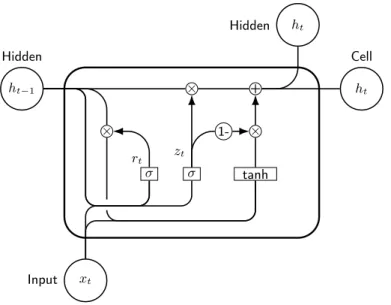
2.7 Recurrent Neural Network (RNN)
When sequential data is used, the order of each item in the sequence is important. For instance, we read sentences word by word in order to make sense of it and if we change the order, the sentence might become unintelligible or actually mean new things that the original sentence does not communicate. An RNN is a neural network with cyclical connections that naturally composes sequential information. Here, hidden layer of the
σ σ tanh σ × + × × tanh ct−1 Cell ht−1 Hidden xt Input ct Cell ht Output ht Hidden ft i t ot Figure 2.3: LSTM structure
current state is calculated by using the previous hidden layer and the current input and this value is the summary of the information given until that point. Formula to calculate the hidden layer of the current state is given as:
ht =tanh(W xt+bx+U ht−1 +bh) (2.23)
where U ∈ Rp×p and W ∈ Rp×m are the parameters matrices, while b{x,h} ∈ Rp are
the related bias vectors with m being the embedding dimension of each word and p
being hidden layer size. Herext is the input vector for current word (or any element
in the sequence) and ht is the hidden layer output of current state, and ht−1 is the hidden layer representation from the previous time step. There are two important variants of RNN used in the deep learning (DL) field.
2.7.1 Vanilla Long Short Term Memory (V-LSTM)
One well known RNN variant we employ in our studies is a standard LSTM, which we hencerforth term V-LSTM. The hidden unit of a V-LSTM model contains an input gate, output gate, and forget gate as shown in Figure 2.3. These gates have a value ranging from 0 and 1 and each gate has a specific role to improve the performance. Input gate controls how much of the new data will be used in current cell, forget gate decides what portion of the previous cell state is needed to be retained, and finally output gate decides how much information from current output will be sent to the next cell. More formally, a V-LSTM is specified as:
it=σ(Wixt+Uiht−1+bi) (2.24) ft =σ(Wfxt+Ufht−1+bf) (2.25) ot=σ(Woxt+Uoht−1+bo) (2.26) ˜ ct =tanh(Wcxt+Ucht−1+bc) (2.27) ct =σ(ftct−1+itc˜t) (2.28) ht=tanh(ct)ot (2.29)
Here, Equations 2.24, 2.25, and 2.26 show the input, forget, and output functions respectively. Equation 2.27 and 2.28 show memory cell equations using input and forget gate. Finally, equation 2.29 calculates the hidden layer of the current V-LSTM unit. it,ft, andotare the input, forget, and output gates respectively. For embedding
dimension of m, and hidden layer size p, U{i,f,o,c} ∈ Rp×p and W{i,f,o,c} ∈ Rp×m are
the parameter matrices while b{i,f,o,c} ∈ Rp are the related bias vectors. Also, σ()
is the sigmoid function and tanh() is the hyperbolic tangent function. Here, xt is
the input vector, ct is the memory cell, and ht is the hidden layer of related LSTM
unit. Our intuition in the context of LEMRs is to represented all structured codes just as one would embed words in a sentence. However, at each time step, there is an entire EMR instead of a single word. To handle this, an EMR can be represented by the simple average of embeddings of all constituent codes. Alternatively, different classes of codes (e.g., diagnoses, medications) can be averaged separately and then concatenated to come up with the fix dimensional embedding for an EMR. This latter approach leads to longer representations due to the separation of different types of codes.
2.7.2 Gated Recurrent Unit (GRU)
Another frequently used variation of the RNN model we employ is the GRU, which contains 2 gates: reset gate and update gate. This model provides comparable pre-diction power while the structure is simpler than the LSTM model. Figure 2.4 shows
× + ht Hidden ht−1 Hidden ht Cell xt Input σ σ tanh × 1-× zt rt
Figure 2.4: GRU structure
the structure of GRU and the formal description is as follows:
zt =σ(Wzxt+Uzht−1+bz) (2.30)
rt=σ(Wrxt+Urht−1+br) (2.31)
˜
ht =tanh(Whxt+rtUhht−1 +bh) (2.32)
ht =ztht−1+ (1−zt)h˜t (2.33)
Equations 2.30, 2.31, 2.32, and 2.33 show how to calculate the reset gate(r), the update gate (z), the intermediate memory unit (˜h), and the hidden layer output (h) respectively, where U{i,f,o,c} and W{i,f,o,c} are the parameter matrices while b{i,f,o,c}
are the related bias vectors. The purpose of training is to learn these matrices and bias vectors. Because of the simpler architecture, GRUs tend to be faster. The representation of EMRs to be processed by GRUs is the same as explained for LSTMs in the previous section.
Chapter 3 On Interestingness Measures for Mining Statistically Significant and Novel Clinical Associations from EMRs
Association rule mining has received significant attention from both the data mining and machine learning communities. While data mining researchers focus more on de-signing efficient algorithms to mine rules from large datasets, the learning community has explored applications of rule mining to classification. A major problem with rule mining algorithms is the explosion of rules even for moderate sized datasets making it very difficult for end users to identify both statistically significant and potentially novel rules that could lead to interesting new insights and hypotheses. Researchers have proposed many domain independent interestingness measures using which, one can rank the rules and potentially glean useful rules from the top ranked ones. How-ever, these measures have not been fully explored for rule mining in clinical datasets owing to the relatively large sizes of the datasets often encountered in healthcare and also due to limited access to domain experts for review/analysis. For this chapter, using an EMR dataset of diagnoses and medications from over three million patient visits to the University of Kentucky medical center and affiliated clinics, we conduct a thorough evaluation of dozens of interestingness measures proposed in data mining lit-erature, including some new composite measures. Using cumulative relevance metrics from information retrieval, we compare these interestingness measures against human judgments obtained from a practicing psychiatrist for association rules involving the depressive disorders class as the consequent.
3.1 Introduction
Association rule mining (ARM (Agrawal and Srikant, 1994)) has emerged as an im-portant methodology to gain insights into large databases of transactions each of which contains a set of items. ARM first gained popularity for market-basket anal-ysis where each transaction consists of a set of products purchased by a customer. Using ARM, rules of the form E ⇒Y are extracted which indicate that a customer that buys a set of items E “tends” to buy items in Y in the same visit. ARs ob-tained for this domain have been used to better design product placement layouts in stores that encourage so called cross-selling among customers. Similar strategies are also being employed by online stores to dynamically generate product recommen-dations based on prior browsing/purchasing history. In the context of biomedicine
and healthcare, ARM has also been applied to EMR data for association analysis among biomedical and clinical variables (Brossette et al., 1998; Ordonez et al., 2006; Wright et al., 2010; Wright et al., 2013). Before we proceed further, we establish some primitives for ARM starting with the notion of a clinical item set.
3.1.1 Notions of Statistical Strength, Novelty, & Interestingness
Statistical significance and novelty are two important and complementary notions that make a rule desirable for further examination. Generally speaking, an AR is deemed statistically significant if its manifestation is not due to random chance. Statistical strength is a measure-specific notion that attributes a gradation or degree to the significance of the rule. Thus, we would at least want a rule to be statistically significant and also prefer for it to have high statistical strength. However, statistically significant ARs may not be meaningful or clinically relevant; even in cases when they are meaningful, they might be too obvious. For example, in our experiments, the association of antidepressants with depressive disorders is statistically significant but is very obvious to most end users. For ARM, the notion of novelty indicates the level of unexpectedness, surprise, or peculiarity associated with a rule. For example, the association between antidepressants and depressive disorders is considered not novel. For our current effort, to keep the terminology simple, novelty implicitly also includes the notion of clinical relevance or plausibility. In data mining literature (Geng and Hamilton, 2006; Shaharanee et al., 2011; Tan et al., 2002; Webb and Vreeken, 2014), “interestingness” has been used as an umbrella term to describe a combination of desirable rule properties including statistical strength and novelty and we employ the same usage for the rest of our chapter. Although novelty is sometimes considered a subjective measure, in this chapter we assess how various interestingness measures model novelty. Next we outline our main contributions.
3.1.2 Our Contributions
Prior results on applying ARM to clinical datasets (Wright et al., 2010; Wright et al., 2013) offer important insights but are based on relatively smaller datasets with a focus on rediscovering known associations already recorded in external knowledge bases. Hence they do not directly assess the novelty of the associations found. Fur-thermore, their evaluations consider only few interestingness measures (up to five) in their experiments and also limit the antecedent of an association to be a singleton. In our current effort
1. We use a dataset of diagnoses and medications from over 3 million patient visits to the UKY medical center and its affiliated clinics to obtain all ARs with singleton consequents and having minimum support 100 and minimum confidence 10%. We do not limit the rule antecedents to be singletons; they can be combinations of both diagnoses and medications.
2. We rank the specific set of rules withdepressive disorders as the consequent using over 40 different interestingness measures including most measures introduced in data mining literature (Geng and Hamilton, 2006) and a few new measures we introduce in this chapter.
3. We obtain manually assigned novelty scores (1 – 5) for the set of rules in the union of top 100 rules from rankings produced by all interesting measures using the help of a practicing psychiatrist (Dr. Rayapati, the domain expert of this effort). We combine these novelty scores and odds ratio lower bounds (from 95% confi-dence intervals) for these rules to compare against all interestingness measures and identify classes of measures that trade-off novelty and statistical strength in con-trasting ways. We also discuss the clinical plausibility of several novel associations identified in our analysis.
The central premise for all our work is to pick specific diseases of interest as conse-quents and identify groups of medications and other conditions (as antecedents) that are associated with them. The associations may themselves manifest due to comor-bidity situations (if antecedents are diseases). They can be indicative of treatment relations or side-effect/adverse-reaction scenarios (if the antecedents are medications). Combinations of medications and diseases as antecedents can represent more nuanced and specific scenarios with high statistical strength.
3.2 AR Mining from Visits Data
ARM has been explained in Section 2.2. From a biomedical perspective, we can filter ARs R(V, σ, γ) choosing interesting and meaningful consequents Y. For example, we can set Y ={NSCLC}, that is, a consequent with just one item, NSCLC, which corresponds to patient visits that had a diagnosis code for NSCLC.
As their name indicates, ARs are essentially associations (or correlations) and do not indicate causality, although they have been known to manifest when there is a causal relationship. ARs are also used as starting points to arrive at potential causal relations (Hill, 1965) using additional retrospective analyses involving confounding
factors (not all of which maybe recorded in a clinical database) or additional prospec-tive experiments such as randomized control trials (which may not be feasible in all situations) (Shadish et al., 2002). We emphasize that the scope of this chapter is assessing rule interestingness measures in the context of ranking large AR sets to enable discovery of interesting associations that can lead to novel hypotheses. Next we discuss the notions of statistical strength, novelty, and interestingness of rules generated by ARM. Here we primarily discuss the clinical dataset and methods used to extract ARs.
3.2.1 Clinical Dataset Used
Our dataset is extracted from all patient visits (≈ 3.25 million) during the ten year period 2004-2013 to the UKY medical center and its affiliated clinics. Each visit transaction consists of medications and diagnoses recorded during a particular patient visit∗. We also removed nearly 12,000 transactions that are very large (with 35 or more elements per visit). Although rare and in this case constituting only 0.3% of the full dataset, presence of such long transactions renders existing approaches to ARM impractical given they all rely on generating frequent item sets as an intermediate step. Thus we are still left with ≈ 3.25 million visits from around 572,000 unique patients. Thus, on average, each patient had about 5.66 visits during the decade. Given the ten year window of the study, we chose to treat different visits by the same patient as giving rise to different transactions. This way, the co-occurrences of medications and diagnoses are guaranteed to have the same time stamp in all our transactions.
The dataset has 11,877 unique ICD-9-CM codes and 1032 unique medication codes byCerner MultumTM Lexicon Plus codes which are also used by CDC for their medical care surveys. Current ARM approaches, even with the advent of “big data” approaches, do not scale well to thousands of unique items for patient visit databases with large transaction sizes especially if the minimum confidence and threshold are chosen to be small, which is critical to surface novel associations; high support and confidence rules may satisfy statistical strength requirements but tend to represent common knowledge for most end users. At lower thresholds, scalability issues mostly arise because of the combinatorial explosion of possible antecedent sets. Further-more, considering all unique codes may not offer enough statistical strength (due to sparsity) or yield informative rules (for manual AR interpretation). For example, ∗Although other variables such as procedures and labs are available, for computationally
researchers might be more interested in knowing statistically significant and novel associations of penicillins with other conditions rather than be subjected to a deluge of weak associations involving specific penicillins such as Amoxicillin, Ampicillin, and Dicloxacillin. However, sparsity issues may be overcome by working with much larger datasets compared to the dataset used in our current effort.
Given above scenarios, we group diagnosis and medication codes using conven-tional approaches. For diagnoses, we use ICD-9 code classes (Healthcare Cost and Utilization Project, n.d.) developed by the HCUP, an affiliate of the AHRQ in the US Department of Health and Human Services. These classes group related codes resulting in 282 classes for the 11,877 codes in our dataset. For example, the HCUP class for cancer of breast groups 13 different ICD-9 codes covering all female breast cancer codes, male breast cancer codes, and a code for personal history of breast cancer. We rolled-up the Multum medication codes using their class hierarchy which resulted in 150 classes (e.g., Penicillins). In each transaction, we then replaced the codes with the corresponding HCUP and Multum classes resulting in a total of 432 unique items (HCUP and Multum classes) populating 3.25 million transactions. 3.2.2 Generating Association Rules
Although there are several efficient implementations that extract frequent item sets (Han et al., 2000; Zaki, 2000), including those that work on big datasets using MapRe-duce (Moens et al., 2013), for our purposes the LCM Ver. 3 by Uno et al. (2005) that exploits a clever combination of bitmaps, prefix trees, and array lists worked best. We used a minimum support σ = 100 and confidence γ = 10% for singleton consequent rule generation. That is, in each AR, we require that the antecedent items and consequent co-occur at least 100 times in over 3 million transactions and at least 10% of the transactions that contain the antecedent set also include the consequent. This is in line with other efforts (Wright et al., 2010; Wright et al., 2013) on applying ARM to clinical datasets. LCM generated nearly 22 million rules for our dataset.
At this point, to evaluate interestingness measures for both statistical strength and novelty, we needed to pick a narrow focus. According to the National Comor-bidity Survey Replication (2001–2003), 68% of adults with mental disorders have medical conditions and 29% with medical conditions have mental disorders (Kessler et al., 2004). A February 2011 Robert Wood Johnson Foundation (RWJF) research synthesis report (Druss and Walker, n.d.) presents evidence that this subgroup of people with mental and medical disorder comorbidities are at significant risk for poor quality of care and high costs. Depressive disorders are one of the most common
mental disorders especially among adults and hence we picked the corresponding HCUP class for our focused study. The depressive disorders HCUP class has sixteen ICD-9 codes, which represent all variants of depression in . Our dataset has 54,923 transactions with a depressive disorder code. Post filtering all rules with depressive disorders as the consequent, we obtained 126,540 rules. Upon on manual observation, many of these rules had antidepressants as an element of the antecedent. Since the presence of this well known drug class that treats depression leads to uninteresting associations, we removed those rules with antidepressants as part of the antecedent, which resulted in 75,465 rules. These are the rules we ranked based on different interestingness measures.
3.3 Assessing Interestingness Measures for Association Rule (AR) Rank-ing
We ranked all the 75,465 rules with depressive disorders as the consequent class using nearly three dozen probability based objective interestingness measures from a recent survey by Geng and Hamilton (Geng and Hamilton, 2006, Table IV). This list includes popular measures such as confidence, lift, conviction, odds ratio, and information gain. Additionally, we added the χ2-measure as it is well known for studying statistically significant associations (Hämäläinen, 2011; Wright et al., 2010). We also introduced some new measures which we describe here.
3.3.1 Additional Interestingness Measures
To model novelty, we introduce the notion of AIRF for a given AR E ⇒ Y. Recall from Chapter 2,R(V, σ, γ) represents the set of ARs for the visit databases V satis-fying minimum support σ and confidenceγ. Let RY ⊆ R(V, σ, γ)be the set of rules with Y as the consequent from the full set of rules, assuming the databaseV,σ, and
γ are fixed. We define
AIRF(E ⇒Y) = P x∈E |RY| |{R: R∈RY ∧ x is in antecedent of R}| |E| .
Inverse rule frequency is analogous to inverse document frequency (IDF) in the TF-IDF term weighting scheme popular in information retrieval. The higher the AIRF of a rule E ⇒ Y, the fewer are the rules that contain elements of E as part of their antecedents – in this sense, rules with higher AIRF are expected to be
novel/peculiar. The rationale for AIRF follows from the justification for IDF (Robert-son, 2004).
Odds ratio (OR) is a well known measure for studying associations in epidemi-ology† and more specifically, the ORLB (Morris and Gardner, 1988) of the 95% confidence interval around sample OR is used as an important measure for assessing statistical significance or lack thereof. ORLB >1indicates a statistically significant association with higher values indicating stronger associations. Our new measures of interestingness for a ruleE ⇒Y include its AIRF,ORLB,
ORLB
log2(|E|+|Y|), and
AIRF ·ORLB
log2(|E|+|Y|), (3.1)
wherelog2(|E|+|Y|)indicates the length of the rule. (Note|Y|= 1 for our purposes and the expression equals 1 for singleton associations where additionally |E| = 1). Given ORLB indicates statistical strength and AIRF models novelty, we combined both in the product measure. Although we support longer rules with |E| > 1, very long rules are not interesting as they capture highly specific scenarios that are not amenable to reasonable interpretation and typically have low support as noted in prior efforts (Hämäläinen, 2011). At the same time we do not want to severely discount long rules. So to prefer smaller rules and dampen the effect of the length on overall interestingness score, we uselog2(|E|+|Y|)in the denominator of the two measures in equation 3.1.
3.3.2 Domain Expert Novelty Assessments
We used ORLB introduced in Section 3.3.1 as a proxy for statistical strength in our final assessment of all interestingness measures given it is routinely considered in biostatistics. The rationale for using ORLB over OR is that ORLB balances assurance that the result is not due to chance with the strength of the estimated effect, considering the variance of the estimator. However, we do not have a similar measure for novelty. Given it is unrealistic to have domain expert assessments on 75,000 rules we combined the top 100 rules from each of the rankings produced by all interesting measures discussed in this section. That is, given M is the set of all †For prospective studies, relative risk (RR) is a more intuitive measure of association strength,
but OR is a symmetric measure that is typically used for retrospective studies and approximates RR for rare outcomes (Rosner, 2015, Chapter 13.3). The advantage of OR over RR is that OR can be validly estimated whether random samples are drawn from the population as a whole, from exposure/risk factor strata, or from outcome strata.
0 0.2 0.4 0.6 0.8 1 0.6 0.8 1 Group–1 abcc Group–2 a a a aGroup–3 b a Group–4 b c Group–5 ab cd eff a Group–6 b c d N ovelty W eight(α) α N D C N + (1 − α ) N D C O
G1 :ORLB G1 :Lif t/Interest G1 :Leverage G1 :AddedV alue G1 :Relative Risk G1 :Certainty F actor
G1 :Y ule0s Q G1 :Y ule0s Y G1 :Conviction G1 :Laplace Correction G1 :Inf ormation Gain G1 :Sebag−Schhoenauer
G1 :Odd M ultiplier G1 :Example and CounterexampleRate G1 :Zhang G2(a) : (log(AIRF)∗ORLB)
G2(b) :Av. Conf idence G2(c) :Accuracy G2(c) :Least Contradiction G3(a) :Klosgen
G3(a) :Gini Index G3(a) :Linear Correlation Coef f icient G3(a) :ChiSquare G3(b) :Cosine
G4(a) :J−measure G4(b) :Jaccard G4(c) : 2W ay Support G5(a) :Rule Count G5(b) : 2W ay support V ariation G5(c) :P iatetsky−Shapiro
G5(d) :Specif icity G5(e) :AIRF∗ORLB G5(f) :Rule Support G5(f) :Recall
G6(a) :AIRF G6(b) :Collective Strength G6(c) :One W ay Support G6(d) :Loevinger
Figure 3.1: Interestingness measure profiles with novelty-statistical strength trade-offs
interestingness measures, human annotations are assigned to the set of rules
[
m∈M
Rank100m (RY), (3.2)
where Rankk
m indicates a function that returns the topk rules (without any
limita-tions on rule length) obtained by ranking using measure m. In addition to this, all singleton antecedents which had an ORLB > 1 were also presented to the domain expert. We did this because singleton associations (|E| = 1) are easier to inter-pret, relatively very few compared to longer rules, and ORLB > 1already indicates statistically significant association.
Novelty ratings were assigned on a scale of 1 to 5 (with 5 indicating most novelty) by a practicing psychiatrist from the university’s department of psychiatry. As we
our purposes includes plausibility. So a rating of 1 for a rule indicates it is a well-known association whose underlying mechanism is also reasonably understood. On the other hand a rating of 5 means it is a highly novel rule that is also clinically plausible although the details of the mechanism may not be as clear as for a rule with rating 1. This is to be expected given high novelty usually also implies that pertinent broad knowledge is lacking (see Section 3.4 for literature search based evidence for this). The assessments are informed by the physician’s general medical knowledge and experiences as a practicing psychiatrist. Besides the actual rules, no other information was provided to the physician, who was requested to provide additional qualitative feedback on associations that were deemed highly novel. We chose the top 100 rule set union from all measures in the interest of domain expert time needed for novelty assessment. This limit has resulted in over 550 rules and we believe choosing larger thresholds could help for future efforts.
3.3.3 Comparison of Interestingness Measures
Next we compare interestingness measures discussed in this section across two dimen-sions, statistical strength and novelty, using rule ORLBs and psychiatrist assigned novelty scores as corresponding proxies, respectively. Using each interestingness mea-sure, we rank all rules in equation 3.2 and any other singletons with anORLB > 1for the depressive disorders consequent. For reviewing convenience for the domain expert and subsequent analysis, we split all these rules into singleton and non-singleton an-tecedent rules. We ended up with a total of 231 singleton rules and 334 non-singleton rules each of which was assigned a novelty score (1–5).
The NDCG (Järvelin and Kekäläinen, 2002, Sections 2.2–2.3) is a popular rank quality metric in information retrieval (IR). It is typically used for search engines to measure thegain in terms of graded relevance of retrieved documents where relevant documents higher up in the ranking are given more weight compared with those that come later in the ranking. For interestingness measure comparison in our effort, we adapt NDCG to suit our purposes and compute normalized discounted cumulative novelty (NDCN) (from expert assigned scores) and normalized discounted cumula-tive ORLB ( NDCO) based on the rule ranking produced according to each measure. Instead of the relevance judgment score of a retrieved document, we used a rule’s novelty score (for NDCN) and ORLB (for NDCO). Besides this replacement of rele-vance scores with novelty and ORLB values, the exact expression used for NDCN and NDCO is identical to that of NDCG (Järvelin and Kekäläinen, 2002, Equation (2)). We then sorted all measures based on the corresponding NDCN and NDCO values to