UC Riverside
UC Riverside Electronic Theses and Dissertations
TitleDemand Forecasting in Power Distribution Systems Using Nonparametric Methods: Kernel Density Estimation and Mixture Density Networks Methods
Permalink https://escholarship.org/uc/item/5bg5q9ws Author Patel, Raj Publication Date 2019 Peer reviewed|Thesis/dissertation
UNIVERSITY OF CALIFORNIA RIVERSIDE
Demand Forecasting in Power Distribution Systems Using Nonparametric Methods: Kernel Density Estimation and Mixture Density Networks
A Thesis submitted in partial satisfaction of the requirements for the degree of
Master of Science in
Electrical Engineering by
Raj Deven Patel September 2019
Thesis Committee:
Dr. Hamidreza Nazaripouya, Co- Chairperson Dr. Hossein Akhavan Hejazi, Co- Chairperson Dr. Hamed Mohsenian-Rad
Dr. Nael Abu-Ghazaleh Dr. Ahmed Eldawy
Copyright by Raj Deven Patel
The Thesis of Raj Deven Patel is approved:
Co-Chairperson
Co-Chairperson
Table of Contents
1 ABSTRACT………..……….……1
2 INTRODUCTION………...…..……….3
3 LITERATURE REVIEW………...………6
3.1 Classification of Load Forecasts………...6
3.2 Point Forecasting………...7
3.3 Probabilistic Forecasting………...10
4 METHODOLOGY………..……….…….…14
4.1 Non- Parametric Model for Probability density estimation..……….…14
4.1.1 Kernel Density Estimation……….………...14
4.1.2 Estimation of smoothing parameters..……….……...………..16
4.1.3 Conditional Probability Estimator.……..………..…..………...17
4.2 Mixture Density Network Model for Conditional Probability Estimation……….………..…….…..…...18
4.2.1 Training and Prediction……….……….………..21
5 VALIDATION………23
5.1 Error Calculation………...23
5.2 Quantile Comparison…….…………..………...………23
5.3 Statistical Analysis Test………..………..…….24
6 RESULTS……….…....26
6.1 Simulation Step………..…...……26
6.2 Forecast………...…27
6.3 Performance………29
7 CONLCUSION……….……34
8 REFERENCES……….…...36
9 APPENDIX ………..40
9.1 MATLAB Code for Kernel Density Estimation..………...40
List of Figures and Tables
Figure 1 Example of Mixture Density Network….……….……….19
Figure 2 Gaussian Kernel density estimation for hour 24…….. ……….27
Figure 3 Actual v/s Forecasted Demand (500 hours shown) for a year using Kernel density estimation and Mixture Density Networks……….………...28
Figure 4 Actual v/s Forecasted Demand (500 hours shown) for a winter using Kernel density estimation and Mixture Density Networks………...28
Figure 5 Example of demand distribution at given time using
KDE…….……….……….………30
Figure 6 Example of demand distribution a given time for 3 Gaussian curves using Mixture Density Network……….……….30 Figure 7 A plot for percentage of errors from each method……...……….31 Figure 8 Q-Q Plot of Errors from the KDE vs Normal Distribution. ..……….…32 Figure 9 Q-Q Plot of Errors from MDN v/s Normal Distribution………..32 Table 1 Errors of Demand Estimation ……….…..29 Table 2 DM test Statistics …………..……….33
1. ABSTRACT
This thesis investigates the applications of non-parametric approaches for probabilistic demand forecasting in power distribution systems. This thesis develops two probabilistic short-term load forecasting models. We implement and evaluate two type of probabilistic forecasting methods namely: kernel density estimation and mixture density networks. In particular we are interested in the study of the features and (any) advantages of using machine learning approaches over the more traditional approaches in probabilistic demand forecasting.
This thesis gives a short-term load forecast of the residential demand with respect to the outside temperature using the probabilistic forecasting methods. The factors impacting the performance and accuracy of the forecasts are evaluated. The historical data for energy consumption generally has multiple seasonality’s associated with it. For more accurate demand forecasting, it is critical to take into account the different seasonality’s in the data and the effect of exogenous variables (temperature) while developing different models. Both the models are trained separately for yearly and seasonal datasets to study the effect of seasonality on forecasting.
Various tests are performed on the models to assess their statistical significance when compared to one another. The comparative assessment between Mixture Density Networks and Kernel Density Estimation also advances the knowledge of applying these techniques to STLF. The proposed approaches are compared with
other benchmark models like ARIMA (1,0,0) model and a neural network which are also trained separately for yearly and seasonal datasets.
2. INTRODUCTION
The problem of electric demand forecasting, also known as load forecasting has long been of interest and investigation by power system operators and utilities. The forecast of the peak demand over various spatiotemporal resolution/ aggregative levels and forecast of demand variations over different horizons from diurnal to seasonal, are examples of the load forecast that has been in use for long in standard operation and planning of the grid.
However, with the growth of renewable resources and a more diversified and complex environment for providing energy services the problem has now faced new dimensions and challenges. The permanence constraints are tighter, and applications are wider, requiring specific set of features. The forecast approaches do not cover all the desired needs, rather the practice is to develop and use tailored forecast methods for different purposes.
The short-term probabilistic forecast of the demand is a prime example of specialized approaches, where there is a growing need, interest, and applications in energy systems operations, particularly in the area of energy resource management. In probabilistic load forecasting, more information on the future load is given, such as possible deviation of the forecast from the expected value, the confidence in a particular forecast. This is in contrast to the conventional point forecasting where a single value (scalar or vector) is predicted at each given instance of the forecast.
Although point forecasting has the advantage of simplicity, both in development and use, it ignores the additional information that could give a clear picture of the demand. In contrast, probabilistic load forecasting presents more information on volatility of the demand. With the increasing uncertainties from both of power supply and demand sides, probabilistic load forecasts, in the form of density functions, have attracted increased attentions, due to their ability to provide more comprehensive information about the future than what point forecasts can do. Recently due to uncertainties in load and generation, stochastic optimization algorithms have been used significantly for solving power system scheduling problem.
The Probabilistic short-term forecasting of residential customers of course faces a great number of challenges as many factors are involved and impact the variability of demand. The demand is dependent on various external factors such as number of people present, different time of the day, temperature outside etc. If historical data is used, there are generally multiple seasonality’s attached to it. Nevertheless,
it is common to consider and/or model only a few (dominant) factors in producing forecasts, e.g. based on measurement availability, and treat the impact of other contributing factors in the forecast error.
In the probabilistic approaches for load forecasting, it is common to assume a particular parametric distribution on the available data to produce the forecast, however, such approaches will not only lead to more errors in a particular
application and removing part of the data information, but also are limited in validity and applicability.
Accordingly, this thesis aims at study of the application and permanence of non-parametric approaches for Short Term Load Forecasting problem We implement and evaluate two types of probabilistic non-parametric models which will forecast the customer demand. The two models implemented in this study are: kernel density estimation and mixture density networks. These two models are separately implemented and tested by using yearly as well as seasonal data. This study is performed on the residential customer dataset.
3. LITERATURE REVIEW
This section presents various forecasting approaches that have been used to forecast the electricity demand. This review focuses on basic understanding of the models and their applications.
3.1. Classification of Load Forecasts
In the context of load forecasting, one of the basic categorizations has been in terms of the horizon of application, i.e. Short-Term Load Forecasting (STLF), Mid-Term Load Forecasting (MTLF) and Long-Mid-Term Load Forecasting (LTLF). Short term load forecasts generally include one hour to one week ahead forecasts. The mid-term load forecasts include around 3 years ahead forecasts whereas long-term load forecasting includes around 10-20 years ahead forecasts. There is no single forecast that can cover all the desired needs of the user. A regular practice is to use different forecast methods for different purposes.
The classification of the forecast approaches is also dependent upon climate and different human activities. Climate in general refers to various natural occurrences like rains, winds, temperature etc. If the prediction is for a short period, in STLF out of all the mentioned occurrences, temperature has the most impact on the consumption of power out of all the other factors and thus most of the research available uses temperature information to create models [1]. Since the temperature cannot be predicted in advance for long periods, other factors also play a significant role in MTLF and LTLF.
3.2 Point Forecasting
The approaches in the current literature that are developed or applied in the context of STLF currently can be divided into point forecasting and probabilistic forecasting. Over the years, many techniques have been used in point forecasting like neural networks, ARIMA, SVR etc. In [2], authors perform a super short-term point forecasting using regression, neural network, ARMA and wavelet transform. Authors develop a new hybrid method to predict the solar output power which requires only historical solar power time series data. In [3], authors perform a univariate time series point load forecasting using four different methods: SVR, ARIMA, kNN and Random Forest. The authors conclude that the kNN and the Random forest algorithm outperforms the other algorithms.
Neural networks are widely used in both point and probabilistic forecasting. Over the years there have been many techniques which have used neural networks or artificial intelligence for short term prediction. In [5], a short-term load forecasting has been performed using an artificial neural network. As the load profile of the customers is different for weekdays and weekends, the neural networks are trained separately for better performance. The forecast results obtained by the authors are then compared to the actual data. The authors concluded that separate analysis for weekdays and weekends gives a better prediction with less forecasting error. A Feed-forward neural network can also be used for forecasting. This approach is generally used when dealing with a nonlinear and multivariate problems in large datasets [6]. The paper showed that artificial neural networks (ANNs) require large
amounts of data, without which, training is inadequate and can result in large errors. Nonetheless, when large datasets are available, the implementation of ANN algorithms always outperforms linear regression and achieves a very high forecasting performance.
A few analysts have showed quantitative case studies to look at and assess the different methods for STLF, bringing about empirical surveys. The authors in [7], focus on Artificial Intelligence with Short Term Load Forecasting. It has a critical analysis and review of about 40 journal papers. On extensive comparison, the authors found that there is a possibility of overfitting in ANN models which is a result of overparameterization or overtraining. This is one of the most common problems when working with neural network. In [8] two techniques have been implemented for demand forecasting namely Artificial neural network and linear regression. These two techniques were evaluated, and it was found that the artificial neural network performs better than the linear regression. However, further in [9], a similar forecast and comparison was performed when artificial neural network is compared with bagged tree regression. Bagged tree regression is a type of regression designed to improve the stability and accuracy of the algorithms used. It was found that the bagged trees regression performs better than the artificial neural network.
There are many different surveys which provide a summary for different forecasting techniques. Many other techniques like extrapolation, ARIMA, exponential smoothing, etc. can also be used for forecasting other than regression
and neural networks. Paper [10] lists and performs a survey on a wide range of techniques and concepts that could be used to model the system and perform demand predictions. It presents the different models used as well as future trends. A 2007 comparative analysis [11] shows a comparison between five different methods. These methods are: autoregressive integrated moving average (ARIMA) modeling, periodic AR modeling, an extension of Holt–Winters exponential smoothing for double seasonality, an alternative exponential smoothing formulation, and a principal component analysis (PCA). A 24-hour ahead forecasting is performed, and the five techniques are compared. The Holt-Winter exponential smoothing for double seasonality is found to perform the best.
The review papers discuss the various methods used in forecasting but in order to create a model it is required to know the dependence of our input data on external factors to establish a relationship. As discussed before, the weather plays an important role in estimating the total demand met to a greater degree of accuracy. In [12], the various factors that affect the accuracy of the forecasts were discussed in detail. These include weather data, time of the day, type of customer, economy of the country. The paper analyzed various statistical and AI techniques for short term load prediction. Another recent paper [13] also discusses the dependence of power data on weather data to perform short term load predictions using fuzzy logic.
3.3 Probabilistic Forecasting
Compared to point forecasting approaches there are less development and less abundance of studies on Probabilistic approaches for probabilistic load forecasting. In 2014, a research by Weron [14] offered a review of the electricity price forecasting which although is not demand forecasting but the research further helped in recognizing that there is very less amount of literature available on probabilistic forecasting. A comparison between point forecasting and probabilistic forecasting can be seen in [15]. This paper presents a comparative study on model selection for probabilistic load forecasting, using point and probabilistic error measures respectively. The authors of the paper concluded that the probabilistic forecasting performs better than the point forecasting by performing a pinball test. However, the results obtained only had a marginal difference between the point forecasting and probabilistic forecasting technique. Since the performance of point and probabilistic forecasting is almost the same, we can say this paper does not provide proper forecast using probabilistic approach.
There are mainly two types of techniques used in forecasting which are parametric and non-parametric approaches. The parametric approach relies on the underlying data distribution whereas, no prior information about the data distribution is needed in the non-parametric approach. One of the prime examples in parametric forecasting is quantile regression. Quantile regression is a type of regression analysis used in statistics and econometrics. In [18], the authors propose a practical methodology to generate probabilistic load forecasts by performing
quantile regression averaging on a set of sister point forecasts. One advantage of quantile regression is that the quantile regression estimates are more robust. The authors then compared the proposed approach with several benchmark methods and concluded that the proposed approach leads to a dominantly better performances measured by the pinball loss function and the Winkler score.
The probabilistic approaches generally employ a non-parametric approach as it does not require the prior knowledge of the data. In paper [16], a method using Gaussian process is designed for residential load forecasting. In this work, probabilistic and deterministic error metrics were evaluated, and several kernels were compared. The estimation of the kernel requires various bandwidth parameters which determine the smoothness and the width of the kernel. It is extremely important to select proper parameters, or the resulting PDF estimate may be incorrect. In [17], a probabilistic load forecasting algorithm considering contingency parameters is developed for the peak load forecasting. Using Anderson-Darling test toolbox in MATLAB and the historical data, the probabilistic distribution of the contingency parameters can be determined. The Monte-Carlo simulation is used to forecast the load scenarios based on the proposed algorithm. It was concluded that the developed algorithm can follow the real scenario with over 95% accuracy.
In a paper [20], a novel approach is proposed, which applies linear quantile regression technique to approximate unknown cumulative distribution of random variables in the hierarchy without any distributional assumptions. The distribution
of all aggregates are computed by using the empirical copulas in order to produce probabilistic coherent forecasts. By combining quantile regression and empirical copulas, the joint distribution of random variables is estimated, which simplifies the prediction procedure and makes it less complicated than the existing methods. Although novel, the training time for this approach is considerably high and thus might be too long to be acceptable.
Probabilistic load forecasting has gained widespread attention in recent years because it presents more uncertainty information about the future loads. In paper [22] a PLF method to leverage existing point load forecasts by modeling the conditional forecast residual is proposed. Specifically, the method firstly conducts point forecasting using the historical load data and related factors to obtain the point forecast. Then, this point forecast is used as an additional input feature to describe the conditional distribution of the residual on the point forecast. Conditional distribution helps to better understand the relationship between the power consumption by the users and the input feature. Finally, the point and the residual forecasts are integrated to produce the final forecast. This method significantly improves the accuracy of the forecast. Overall, it is evident that the probabilistic forecasting approach is a more powerful tool as compared with point forecasting. Also, in probabilistic forecasting, we prefer to use the non-parametric methods over the parametric methods because it requires no prior information about the data distribution.
This thesis develops a forecasting model based on probabilistic non-parametric methods to predict the daily aggregate consumption of a class of customers by estimating the conditional probability at a given time and temperature. These above-mentioned methods in the literature face a series of challenges in forecasting as there is no proper profile for consumption of electricity by the users. As known, the electricity consumption largely depends upon external factors which includes outside temperature and time of the day. To perform the prediction, historical data is needed through which we can estimate the conditional probability of the output power (demand) with respect to a given temperature for a given time of the day.
The methods mentioned in this paper allows a PDF to be estimated by kernel density estimation method and mixture density networks from a dataset without making any assumption on population properties. It is possible to create an effective model from the survey data that shows the temperature dependence. This thesis describes how to develop such models and use them for demand estimation.
4. METHODOLOGY
The conditional probability of the demand with temperature is estimated. Two models are created, implemented and compared. The first model is called kernel density estimation model and the second model is called a mixture density network model. These models provide the conditional probability of demand at any given temperature and time.
4.1 Non-Parametric Kernel Estimation Model for Probability density estimation
This method creates a model between the residential customer demand, temperature and the time of the day. It helps the estimation of the PDF without making any population property assumptions.
There is a variation in demand at any given time. This demand is random and can vary from day to day. The variation in demand for a residential customer depends mainly on the weather factors (majorly temperature). Thus, a bivariate PDF of demand and temperature can be used to describe the demand at a given time. In order to create a PDF, we make use of the method of Kernel Density Estimation.
4.1.1 Kernel Density Estimation
Kernel density estimation is a fundamental data smoothing problem where inferences about the population are made, based on a finite data sample. This kernel density estimation is for univariate data as well as bivariate data.
There are many different kernel density functions that can be used to estimate the PDF. Some of the kernel density functions include: uniform, triangular, triweight,
Epanechnikov, Gaussian etc. All these different kernel density functions have different tradeoffs such as the Epanechnikov kernel is optimal in a mean square error sense [32]. In this approach we use a gaussian kernel density function to estimate the PDF between temperature and demand.
For each hour we estimate a gaussian kernel density PDF as in [3] using (1):
f (p, T) = ∑ exp [(𝑝 − 𝑝(𝑡) 2ℎ𝑝2(𝑡)) − ( 𝑇 − 𝑇(𝑡) 2ℎ𝑡2(𝑡))] 𝑛 𝑖=0 2𝜋𝑛ℎ𝑝ℎ𝑡 (1) where
p(t) = power demand (from the data) T(t) = temperature (from the data)
hp(t) = Smoothing parameter for demand data
ht(t) = Smoothing parameter for temperature data
n = number of days
The Gaussian kernel density can be calculated as shown above. However, there is still a need to estimate the smoothing parameters for the data before we begin with estimation of the PDF.
4.1.2 Estimation of Smoothing Parameters (Bandwidth Selection)
The bandwidth or the smoothing parameters of the kernel has a very strong influence on the estimate of the PDF. In practice one can say that if the smoothing parameters are larger, we get a general and a smooth shaped PDF estimate whereas if the parameters are smaller, we get a PDF which may not be as smooth as the previous case, but it reveals all the local properties. The selected parameters can be validated once the PDF curve is obtained through cross validation. The initial smoothing parameters can be found by using [3] in (2) and (3): ℎ𝑝(𝑡) = 𝜎(𝑡)(1 − 𝜌2(𝑡))5⁄12(1 +𝜌 2(𝑡) 2 ) −1 6 ⁄ 𝑛−1⁄6 (2) ℎ𝑡(𝑡) = 𝜎(𝑡)(1 − 𝜌2(𝑡))5⁄12(1 +𝜌 2(𝑡) 2 ) −1 6 ⁄ 𝑛−1⁄6 (3) where
σp = standard deviation for demand at time t
σt = standard deviation for temperature at time t
ρ = correlation coefficient calculated at time t
Once all the smoothing parameters are calculated, (1) can be used to estimate the gaussian kernel density function.
Next, the limits for the demand are calculated. These limits are determined from the sample as shown below in (4) and (5):
𝑝𝑚𝑎𝑥 = min{𝑝𝑚𝑎𝑥(𝑡), 𝑝𝑎𝑣𝑔(𝑡) + 3.5𝜎𝑡(𝑡)} (5)
where
pmin(t) = minimum demand at time t
pmax(t) = maximum demand at time t
pavg(t) = average demand at time t
This method used in (4) and (5) calculates the limits based on standard deviation, assuming a normal distribution of the demand.
4.1.3 Conditional Probability Estimator (Demand Estimation)
Having the gaussian kernel density estimate of demand at any given temperature Tt, the conditional distribution is given as follows:
𝑓𝑡(𝑝 𝑇⁄ ) = 𝑐. 𝑓𝑡 𝑡(𝑝, 𝑇𝑡) (6)
where c is a constant calculated from the following condition
∑ 𝑓𝑡(𝑝 𝑇⁄ ) = 1𝑡 𝑃𝑚𝑎𝑥
𝑃𝑚𝑖𝑛
(7)
From the above given equations, we can calculate the conditional probability for any given time and temperature.
Once the distribution of demand at a given time and temperature is available, the expected demand can be calculated as the expectation of the conditional probability which is given as in (8):
𝑝̂ = 𝐸(𝑝 𝑇⁄ ) = ∫ 𝑝. 𝑓𝑡 𝑡(𝑝 𝑇⁄ ). 𝑑𝑝𝑡 𝑃𝑚𝑎𝑥
𝑃𝑚𝑖𝑛
(8)
4.2 Mixture Density Networks for Conditional Probability Estimation
The Mixture Density Networks can be implemented using neural networks where a custom layer of neurons is trained to learn the conditional probability density functions. The probability density of the target data is then represented as a linear combination of kernel functions in the form:
𝑓(𝑝 𝑡⁄ ) = ∑ 𝛼𝑖
𝑚
𝑖=1
(𝑡)∅𝑖(𝑝 𝑡⁄ ) (9)
where m = number of mixture components which is a user defined parameter p = target data/demand data
t = input data/temperature data
𝛼𝑖(x) = mixing coefficients
And ∅(𝑝 𝑡⁄ ) is the conditional density of the target vector for the ith kernel. Gaussian
kernel function has been used in this method to estimate the conditional probability which is obtained from (10):
∅
𝑖(𝑝 𝑡
⁄ ) =
1
√(2𝜋)𝜎
𝑖(𝑡)
2𝑒𝑥𝑝 {−
||𝑝 − 𝜇
𝑖||
22𝜎
𝑖(𝑡)
2}
(10)
Where 𝜇𝑖 represents the center of the ith kernel.
𝜎𝑖 is the variance of the ith kernel.
For any given value of t, the mixture model provides a general formalism for modelling an arbitrary conditional density function 𝑝(𝑝 𝑡⁄ ). We now take the various
parameters of the mixture model, namely the mixing coefficients 𝛼𝑖(t), the means
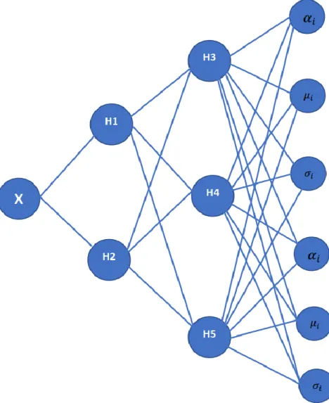
𝜇𝑖(t) and the variances 𝜎𝑖(t), to be general (continuous) functions of t. This is achieved by modelling them using the outputs of a conventional neural network which takes t as its input. The combined structure of a feed-forward network and a mixture model we refer to as a Mixture Density Network (MDN) is shown in figure 1 below [10].
In this approach we have a hidden layer of sigmoidal units and the output layer of linear units zj. The total number of network outputs are (c+2) *m instead of the
usual c outputs.
Now since 𝛼𝑖(x) represents the mixing coefficients (or the priori probability), it must satisfy the constraint:
∑ 𝛼𝑖(t) 𝑚
𝑖=1
= 1
(11)
This is achieved by introducing the softmax function to the network outputs
𝛼
𝑖=
exp(𝑧
𝑖𝛼
)
∑
𝑀𝑗=1exp(𝑧
𝑗𝛼)
(12)
Where 𝑧𝑖𝛼 is the corresponding network outputs. Since the variances are the scale parameters, they are represented as the exponentials of the corresponding network outputs.
𝜎𝑖 = exp(𝑧𝑖𝜎) (13)
The centers 𝜇𝑖 represent location parameters that are directly represented by the network outputs
The error function for the network is defined as the negative log likelihood function which is given as follows:
𝐸𝑞 = −log{∑𝛼 𝑖 𝑚
𝑖=1
(𝑡𝑞)∅𝑖(𝑝𝑞⁄ )} 𝑡𝑞 (15)
is the contribution of error from each pattern q. The total error is given as 𝐸 = ∑𝐸𝑞 (16) 4.2.1 Training and Prediction
From the input and the target data given, the goal is to predict the conditional probability of demand in kW at a given temperature and time. Thus, we need a total of 24 neural networks to predict the conditional density at any given hour based on temperature.
A neural network model is created according to the above conditions (13), (14) and (15) for hour 1. The temperature is taken as the input data and the demand in kW as the target data. Further the variances are now represented using an Exponential Linear Unit (ELU) model with an offset. ELU being a monotonic function with an offset never allows the variances of the distribution to be negative. Thus, we end up with the following transformation.
𝜎𝑖 = ELU(𝑧𝑖𝜎) + 1 (17) The neural network with 800 neurons, 2 layers and the 3 gaussian curves is then trained for 1000 epochs to predict the distribution parameters corresponding to the
target. These parameters are found to be optimal after many trial and errors methods by varying these parameters and training the neural network.
Similarly, all the remaining neural networks (23) for all other hours of the day are created and trained in a similar way. Once all the networks are trained and ready the conditional probability can be predicted.
The input data (temperature) is given as the input to the neural network. The neural network generates distribution parameters for the underlying gaussian curves. These parameters are then substituted in (7) and (8) to get the conditional density function. Since the maximum probability never exceeds one, the following condition must be satisfied.
∫𝑃𝑚𝑖𝑛𝑃𝑚𝑎𝑥𝑓(𝑝 𝑡⁄ ). 𝑑𝑝 = 1 (18)
The expected demand can be easily calculated as shown:
𝑝̂ = 𝐸(𝑝 𝑇⁄ ) = ∫ 𝑝. 𝑓𝑡 𝑡(𝑝 𝑇⁄ ). 𝑑𝑝𝑡 𝑃𝑚𝑎𝑥
𝑃𝑚𝑖𝑛
(19)
5. VALIDATION 5.1 Error Calculation
The Relative Root Mean Square Error (RRMSE) is used to measure the error over the given data by comparing the estimated demand with actual demand. The RRMSE is calculated as shown below in (20):
𝑅𝑅𝑀𝑆𝐸 = √∑ (𝑃(𝑡) − 𝑃̂(𝑡)) 2 𝑁 𝑡=1 ∑𝑁 𝑃2(𝑡) 𝑡=1 (20)
Where 𝑃(𝑡) is the actual demand and 𝑃̂(𝑡) is the predicted demand, t is time and N is the total number of hours.Further Mean Absolute Percentage Error was also calculated for the error evaluation. It is given as in (21):
𝑀𝐴𝑃𝐸 = 1 𝑁 ∑ | 𝑃(𝑡)−𝑃̂(𝑡) 𝑃(𝑡) | 𝑁 𝑡=1 (21)
The power has been predicted using both the methods mentioned above and the results are compared in the next section.
5.2 Quantile Comparison
For the comparison of error quantiles, a Q-Q plot of the errors from both the models is created. A Q-Q plot is a scatterplot created by plotting two sets of quantiles against each other. The steps to generate a Q-Q plot are straightforward. First, each data point needs to be given its own quantile. The set of intervals of the quantiles are chosen based on the data. Next, take a normal curve and add the
same interval of the quantiles that were chosen for the input data. Now, plot each of the point from first data set with respect to the point from normal curve in the given quantile range. Each y coordinate on this plot corresponds to one of the quantiles of the distribution plotted against the quantiles of the normal distribution. If both the sets are from the same distribution, we get a straight line for the Q-Q plot.
5.3 Statistical Analysis Test
The need for formal tests for comparing predictive accuracy is necessary but most methods have no considerations of the statistical significance. Such comparisons are incomplete. A statistical analysis of both the models is performed to determine which one of the models has a better performance. This test used in this analysis is called the Diebold- Mariano (DM) Test.
The essence of the DM approach is to take forecast errors as primitives, intentionally, and to make assumptions directly on those forecast errors. First, the residual (or errors) for both the methods should be calculated. Next, a differential is defined as the difference between square of the residuals from first and second method. Once the value of the differential is calculated, the values of DM statistic are then calculated based on the errors of the model as shown in (19). The models are scored against one another and the model which obtains the highest score is considered to outperform the other model. However, only two models can be compared at one time using this test.
𝐷𝑀 = 𝑑̅
√[γ+2 ∑ℎ−1𝑘=1 ] γ 𝑛
(22)
6. RESULTS
6.1 Simulation Setup
The research uses the dataset provided in GEFCOM12. The dataset consists of hourly observations of temperature in Fahrenheit and corresponding demand in Watts.
For these models a full year of data has been used for training the model. In case of kernel density estimation this historical data has been used to estimate the joint PDF of demand and temperature at any given time. This estimate is later used to calculate the forecasted demand using probability.
In case of mixture density networks, the temperature is given to the neural network as the input data and demand as the target data. The chosen neural network for the model has 800 neurons, 2 layers and 3 outputs for gaussian curves.
It is known that the demand profile for the customer depends on outside temperature and time of the day. However, we can also see the effect of seasonality. For instance, in summer the collective use of air conditioning can contribute to the overall demand, whereas in winter it could be due to the use of heaters. It is easier to capture this trend if the models are trained by keeping seasonality in mind. The consumption profile of customers is expected to be similar from seasons to season. A different model is created using both the methods to account for seasonality. These models use two years of seasonal data to train the models in each case.
The testing for the forecasts is performed for the next subsequent year when the whole year is taken into account whereas seasonal testing is performed on subsequent seasons of the subsequent year.
Reported Parameters for Joint Probability Kernel Density Estimation
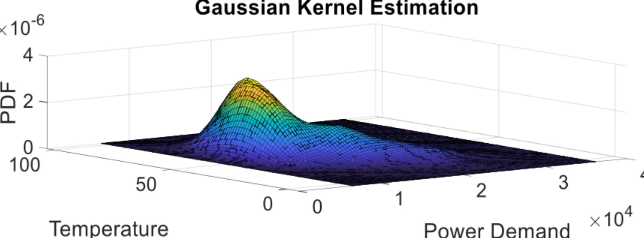
A joint PDF is estimated between demand and temperature for each hour of the day. A gaussian kernel density estimate can be found by using (1). In order to estimate the gaussian kernel density, smoothing parameters are also required. These parameters can be calculated from (2) and (3). The PDF is generated using gaussian kernel with parameters ℎ𝑝 = 1.49 and ℎ𝑡 = 7.7171 F. Figure 2 shows the implemented gaussian kernel for hour 24 using the reported parameters.
Figure 2: Gaussian Kernel density estimation for hour 24 6.2 Forecast
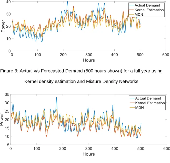
Figure 3 shows the actual and the forecasted demand for a whole year using the kernel density estimation model and mixture density function. The training of the model is performed for the whole previous year.
Figure 4 shows the actual and the forecasted demand for the winter month of the year using the kernel density estimation model and mixture density networks. The training of the model is performed for the winter seasons of the previous two years.
Figure 3: Actual v/s Forecasted Demand (500 hours shown) for a full year using Kernel density estimation and Mixture Density Networks
Figure 4: Actual v/s Forecasted Demand (500 hours shown) for a full winter using Kernel density estimation and Mixture Density Networks.
6.3 Performance
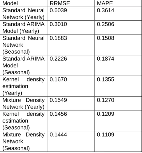
The estimation results were compared to the actual demands. Table 1 shows the RRMSE and MAPE values for both the models for yearly as well as seasonal training on data. The table compares the error values generated from the implemented model to the standard benchmark models in Matlab. A Neural network with 1000 neurons and ARIMA model (1,0,0) were implemented as a part of the benchmark.
TABLE 1: Errors of Demand Estimation
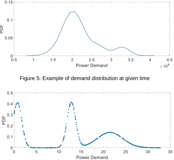
From (5) and (6), the conditional probability for any given time and temperature can be calculated. Figure 6 shows the conditional probability of power demand
Model RRMSE MAPE
Standard Neural Network (Yearly) 0.6039 0.3614 Standard ARIMA Model (Yearly) 0.3010 0.2506 Standard Neural Network (Seasonal) 0.1883 0.1508 Standard ARIMA Model (Seasonal) 0.2226 0.1874 Kernel density estimation (Yearly) 0.1670 0.1355 Mixture Density Network (Yearly) 0.1549 0.1270 Kernel density estimation (Seasonal) 0.1456 0.1209 Mixture Density Network (Seasonal) 0.1444 0.1109
with temperature at a particular given time of the day (For e.g. 8 pm) using the kernel density estimation method. Figure 6 shows an example of conditional distribution of demand with temperature at a particular time of the day with the assumption of 3 gaussian curves using Mixture Density Networks.
Figure 5: Example of demand distribution at given time
Figure 6: Example of demand distribution a given time for 3 Gaussian curves using Mixture Density Network
6.4 Analysis
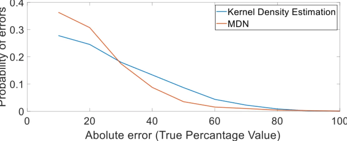
After the forecasts and error matrix is generated, it is seen in Table 1 that both the models perform better than the benchmark models. It is also seen from the table that the Mixture Density Network model performs better than the kernel density estimation method. However, it is not yet completely possible to determine which model performs better than the other. So, we perform some extra tests that help us understand the statistical significance of both the models. The following plot shows the distribution of probability of errors from both the implemented methods. These errors are plotted over the percentage values according to the ascending order.
Figure 7: A plot for Number of errors from each method Q-Q Plot
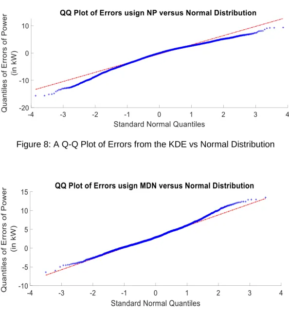
This test is performed to visualize the nature of the error. The nature of error (or noise) ideally is normal in nature (white noise). So ideally, errors from both the models must belong to the normal distribution. Although errors both the models
errors from the MDN follow a closer normal distribution than the errors from KDE model.
Figure 8: A Q-Q Plot of Errors from the KDE vs Normal Distribution
Diebold-Mariano Test
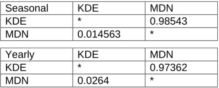
The above figures are still not enough to say that the mixture density network forecast is better than kernel density estimation forecast. The D-M test however gives the statistical analysis of the models as seen in the table below. On comparing both the models for yearly and seasonal dataset, we can see from the Mixture Density Network model outperforms the kernel density estimation model.
TABLE 2: DM test Statistics
Seasonal KDE MDN KDE * 0.98543 MDN 0.014563 * Yearly KDE MDN KDE * 0.97362 MDN 0.0264 *
7. CONCLUSION
The goal of this thesis was to perform probabilistic demand forecasting using non-parametric methods and compare them. The forecasting approaches implemented are based on the temperature dependence of the demand. While forecasting, temperature data is given as the input to the system to forecast the demand. The Non-parametric methods for probability estimation helps us in constructing models which have only temperature dependence. Since a non-parametric method is applied, there is no need for prior analysis of the data i.e., there is no need to make assumptions about the population. The kernel density estimation model and the mixture network density model were implemented under these methods. The Kernel Density Estimation method estimates the joint PDF between demand and temperature at any given time whereas the Mixture Density Networks estimates the distribution parameters for a Gaussian Kernel by using a neural network. We address several challenges in the implementation of the two models. We address the challenges of overfitting, range selection, training time, bandwidth selection, parameter selection for neural networks.
In kernel density estimation method, it is important to select proper range of inputs for power and temperature during the construction of the joint PDF. If we select a wide range of inputs, then our model may capture extra information for the joint PDF which is not desirable and if the input range is very narrow, there is a chance that the model does not capture the desired information for kernel density estimation. Another challenge in this method is the selection of bandwidth
parameters for kernel density estimation which determine the width of the estimated PDF.
In Mixture density networks method, there is a challenge of overfitting of data. This can be avoided by choosing the proper parameters for the neural networks. If we have too many neurons and layers, it can result in overfitting whereas too less of it can cause underfitting. These parameters also affect the training time of the networks. Since both the methods are data driven it ensure the portability of the methods.
During training of the neural networks, it was found that there is a trade-off between number of neurons, hidden layers and the overall accuracy. Also, it can be seen from the results that there is an improvement in the model accuracy when the seasonality is considered over the yearly dataset. This is because when seasonality is considered it is possible to capture the minute variations. In future, we can also implement and compare the same models on weekdays and weekends customer profiles separately.
Since there isn’t much work done on probabilistic demand forecasting using
mixture density networks, this research provides a foundation for the same. The current dataset has hourly observations for temperature and demand, it would be interesting to see how the accuracy of the models change with change in dataset and time intervals.
8. REFERENCES
[1] Tao Hong (2011), Short Term Electric Load Forecasting (Doctoral Dissertation)
[2] H. Nazaripouya, B. Wang, Y. Wang, P. Chu, H. R. Pota and R. Gadh, "Univariate time series prediction of solar power using a hybrid wavelet-ARMA-NARX prediction method," 2016 IEEE/PES Transmission and Distribution Conference and Exposition (T&D), Dallas, TX, 2016, pp. 1-5. [3] M. Majidpour, H. Nazaripouya, C. Chu, H. R. Pota, and R. Gadh, "Fast
Univariate Time Series Prediction of Solar Power for Real-Time Control of Energy Storage System ", in Forecasting, vol. 1, pp. 107-120, Sept. 2018.
[4] W. Charytoniuk, M.S. Chen, P. Kotas, and P. Van Olinda, “Demand Forecasting in Power Distribution Systems Using Nonparametric
Probability Density Estimation”, IEEE Transactions on Power Systems, Vol 14, No. 4, November 1999.
[5] Saurabh Singh, Shoeb Hussain, Mohammad Abid Bazaz (2017). “Short-term load forecasting using Artificial Neural Network.” Proceedings of the IEEE, 75, 1558–1573.
[6] Jonathan Schachter & Pierluigi Mancarella. (2014). “A Short-term Load Forecasting Model for Demand Response Applications”. 11th International Conference on the European Energy Market (EEM14).
[7] Hippert, H. S., Pedreira, C. E., & Souza, R. C. (2001). “Neural networks for short-term load forecasting: A review and evaluation.” IEEE Transactions on Power Systems, 16, 44–55.
[8] Sharad Kumar, Shashank Mihra, & Shashank Gupta. (2016). “Short Term Load Forecasting using ANN and Multiple Linear Regression”.
[9] Vasudev Dehalwar, Akhtar Kalam, Mohan Lal Kolhe, Aladin Zayegh. (2016). “Electricity load forecasting for urban area using weather forecast information”. 2016 IEEE International Conference on Power and Renewable Energy.
[10] Luis Hernandez, Carlos Baladr´ on, Javier M. Aguiar, Bel´ en Carro, Antonio J. Sanchez-Esguevillas, Jaime Lloret, and Joaquim Massana. “A Survey on Electric Power Demand Forecasting: Future Trends in Smart Grids, Microgrids and Smart Buildings”. IEEE Communications Surveys &
[11] Taylor, J. W., & McSharry, P. E. (2007). Short-term load forecasting methods: An evaluation based on European data. IEEE Transactions on Power Systems, 22, 2213–2219.
[12] Feinberg, E. A., & Genethliou, D. (2005). Load forecasting. In Applied mathematics for restructured electric power systems: optimization, control, and computational intelligence (pp. 269–285).
[13] P Mukhopadhyay, G. Mitra, S. Banerjee, & G. Mukherjee. (2017). “Electricity Load Forecasting Using Fuzzy Logic Short Term Load Forecasting Factoring Weather Parameter”.
[14] Rafal Weron. “Electricity price forecasting: A review of the state-of-the-art with a look into the future”. International Journal of Forecasting 30 (2014). [15] Jingrui Xie., and Tao Hong (2016). “Comparing Two Model Selection
Frameworks for Probabilistic Load Forecasting”. 2016 International Conference on Probabilistic Methods Applied to Power Systems.
[16] Mahmoud Shepero, Dennis van der Meer, Joakim Munkhammar and Joakim Widén. “Residential probabilistic load forecasting: A method using gaussian process designed for electric load data”, Appl Energy 218 (2018)159–172.
[17] Md Nasmus Sakib Khan Shabbir, Mohammad Zawad Ali, Muhammad Sifatul Alam Chowdhury, and Xiaodong Liang. “A Probabilistic for Peak Load Demand Forecasting”. 2018 IEEE Canadian Conference on Electrical & Computer Engineering (CCECE).
[18] Bidong Liu, Jakub Nowotarski, Tao Hong, and Rafał Weron. “Probabilistic Load Forecasting via Quantile Regression Averaging on Sister Forecasts.”. IEEE Transactions on Smart Grid, vol. 8, no. 2, March 2017
[19] Jingrui Xie; Tao Hong and Chongqing Kang. “From High-resolution Data to High-resolution Probabilistic Load Forecasts”. 2016 IEEE/PES Transmission and Distribution Conference and Exposition (T&D).
[20] Tianhui Zhao, Jianxue Wang and Tao Zhang (2019). “Day-Ahead Hierarchical Probabilistic Load Forecasting with Linear Quantile Regression and Empirical Copulas”. Volume 7, 2019 IEEE Access.
[21] Mehdi Rafiei, Taher Niknam, Jamshid Aghaei, Miadreza Shafie-Khah and João P. S. Catalão. “Probabilistic Load Forecasting Using an Improved
Machine”. IEEE TRANSACTIONS ON SMART GRID, VOL. 9, NO. 6, NOVEMBER 2018
[22] Yi Wang, Ning Zhang, Yushi Tan, Tao Hong, Daniel S. Kirschen and Chongqing Kang. “Combining Probabilistic Load Forecasts”. IEEE TRANSACTIONS ON SMART GRID, VOL. 10, NO. 4, JULY 2019.
[23] Hyndman, R. J., & Fan, S. (2010). “Density forecasting for long-term peak electricity demand.” IEEE Transactions on Power Systems, 25, 1142–1153. [24] Yi Wang, Qixin Chen, Ning Zhang and Yishen Wang. “Conditional Residual Modeling for Probabilistic Load Forecasting”. IEEE Transactions on Power Systems, vol. 33, no. 6, November 2018
[25] Khotanzad, A., & Afkhami-Rohani, R. (1998). ANNSTLF—Artificial neural network short-term load forecaster generation three. IEEE Transactions on Power Systems, 13(4), 1413–1422.
[26] Jingrui Xie., and Tao Hong (2016). “Comparing Two Model Selection Frameworks for Probabilistic Load Forecasting”. 2016 Interntional Conference on Probabilistic Methods Applied to Power Systems.
[27] Christopher M. Bishop, “Mixture Density Networks”. 1994
[28] Weron, R. (2006). Modeling and forecasting electricity load and prices a statistical approach. Wiley.
[29] Taylor, J. W., & McSharry, P. E. (2007). Short-term load forecasting methods: An evaluation based on European data. IEEE Transactions on Power Systems, 22, 2213–2219.
[30] Feinberg, E. A., & Genethliou, D. (2005). Load forecasting. In Applied mathematics for restructured electric power systems: optimization, control, and computational intelligence (pp. 269–285).
[31] Khotanzad, A., & Afkhami-Rohani, R. (1998). ANNSTLF—Artificial neural network short-term load forecaster generation three. IEEE Transactions on Power Systems, 13(4), 1413–1422
[32] “Kernel Density Estimation”. [Online]. Available: https://en.wikipedia.org/wiki/Kernel_density_estimation
[33] T. Hong, P. Pinson, and S. Fan, “Global energy forecasting competition 2012,” Int. J. Forecast., vol. 30, no. 2, pp. 357–363, 2014.
[34] “A Hitchhiker’s Guide to Mixture Density Networks.” [Online]. Available: https://towardsdatascience.com/a-hitchhikers-guide-to-mixture-density-networks-76b435826cca.
[35] “Mixture-Density-Networks-for-distribution-and-uncertainty-estimation.” [Online]. Available: https://github.com/axelbrando/Mixture-Density-Networks-for-distribution-and-uncertainty-estimation.
9. APPENDIX
9.1 MATLAB CODE FOR NONPARAMETRIC PROBABILITY DENSITY ESTIMATION
Read the temperature and the power data for the entire training duration. Let the data be of the univariate time-series form where for each temperature observation, a corresponding reading for power in kW is available.
Once we have the data available, we use it to determine the smoothing parameters using the following function which takes power data, temperature data and the number of days as the input and produces the smoothing parameters for power and temperature as the output respectively.
function [hp, ht]= smoothing_parameters(class, temp,days) i=1; i1=1; h=1; count=1; a=1; for count=1:24 gg=zeros(days,1); ggg=zeros(days,1); a=1; for i=count:24:length(class) gg(a) = temp(i,2);
ggg(a) = class(i,2); a=a+1; end cc = corr2(gg,ggg); cc(isnan(cc))=0; hp(count,1) = count; ht(count,1) = count; sdp = std(ggg); sdt = std(gg); hp(count,2) = (sdp)*((1-(cc^2))^(5/12))*(1+((cc^2)/2))*(days^(-1/6)); ht(count,2) = (sdt)*((1-(cc^2))^(5/12))*(1+((cc^2)/2))*(days^(-1/6)); end for i=count:24:length(class) gg(a) = temp(i,2); ggg(a) = class(i,2); a=a+1; end cc = corr2(gg,ggg); cc(isnan(cc))=0; hp(count,1) = count; ht(count,1) = count;
sdp = std(ggg); sdt = std(gg);
hp(count,2) = (sdp)*((1-(cc^2))^(5/12))*(1+((cc^2)/2))*(days^(-1/6)); ht(count,2) = (sdt)*((1-(cc^2))^(5/12))*(1+((cc^2)/2))*(days^(-1/6)); end
Next, we use the parameters to generate a gaussian kernel using the following function
function [f,x]=gaussiankernel3(class,hp,ht,temp) %Gaussian Kernel Density Estimation
for j=4:27 gg(:,1) = class(1:end,j); gg(:,2) = temp(1:end,j); [f{j-3},x{j-3}] = ksdensity(gg,"Bandwidth",[hp(j-3,2) ht(j-3,2)]); % figure ksdensity(gg,"Bandwidth",[hp(j-3,2) ht(j-3,2)]); title('Gaussian Kernel Estimation')
xlabel('Power Demand') ylabel('Temperature') zlabel('PDF')
end end
The following function is used to generate the limits for demand function [max1,min1] = maxmin1(class)
i1=1; h=1; count=1; a=1; for count=1:24 for i=count:24:length(class) ggg(a) = class(i,2); a=a+1; end pmin = min(ggg); pavg = mean(ggg); pmax = max(ggg); sdp = std(ggg); min1(count,2) = min(pmin,(pavg-sdp)); max1(count,2) = max(pmax,(pavg+sdp)); min1(count,1) = count; max1(count,1) = count; end
This function takes inputs as the PDF function generated using the gaussian kernel and the limits for demand as the input and generates the constant for conditional probability at different temperature matrix as the output.
function[const temp] = condtn(pout,xin,max1,min1) count =0; for i=1:30 for j=1:24 minval = min1(j,2); maxval = max1(j,2); ans=abs((minval)-xin{j}(:,1)); [mval index] = min(ans);
[mxval indexm] = min(abs((maxval)-xin{j}(:,1))); sm=0; for k = index:30:indexm sm = sm + pout{j}(k+count); end temp(j,i) = xin{j}(index+count,2); condt(j,i) = sm; end count = count+1; end
const = 1./condt;
The following function generates the expected power demand model
corresponding to the constant of conditional probability generated at different temperatures. function [np]=npw1(pout,xin,max1,min1,const1) for count = 1:30 for k =1:24 minval = min1(k,2); maxval = max1(k,2); ans=abs((minval)-xin{k}(:,1)); [mval index] = min(ans);
[mxval indexm] = min(abs((maxval)-xin{k}(:,1))); b=count-1; j=1; for i=index:30:indexm g(j) = pout{k}(i+b); p(j) = xin{k}(i+b,1); h(j) = xin{k}(i+b,1); j=j+1; end p=p';
g=g'; h=h'; w=g.*const1(k,count); plot (h,w); tempval=p.*w; np(k,count) = sum(tempval); end end
Once the model is generated, we can use it predict and calculate the performance on new test data.
function [class_error] = cerror(class,temp1,temp2,np) for count=1:24 tmpvar=0; j=0; b=count-1; for i=1:length(temp1) if (i>24) index = mod(i,24); else index = i;
end if (index==0) index =24; end val = temp1(i,2); ans1=abs((val)-temp2(index,:)); [mxval indexm] = min(ans1);
tmpvar(i) = class_mean*np(index,indexm); temperature(i) = temp2(index,indexm); aa(i) = np(index,indexm); end %Calculate RMSE tot=0; tot1=0; for i=1:length(class) a= isnan(tmpvar(i)); if (a==0) tt=(class(i,3)-tmpvar(i))^2; dt=class(i,3)^2; tot=tot+tt; tot1=tot1+dt; end
end
class_error = tot/tot1;
class_error = sqrt(class_error);
9.2 CODE FOR PROBABILITY ESTIMATION USING MIXTURE DENSITY NETWORKS
Let the data be of the univariate form where we have temperature observation for each hour for all days and a corresponding reading for power in kW is available. We need to generate 24 separate neural networks corresponding to each hour of the day. Implementation of one such network is shown below
from __future__ import absolute_import, division, print_function import numpy as np
import tensorflow as tf
import tensorflow.keras as K
from keras.models import Sequential from keras import utils as np_utils
from tensorflow_probability import distributions as tfd
from tensorflow.keras.layers import Input, Dense, Activation, Concatenate
from tensorflow.keras.callbacks import EarlyStopping, TensorBoard, ReduceLROnPlateau
from sklearn.model_selection import train_test_split from sklearn.preprocessing import MinMaxScaler import xlrd
import numpy as np
##This function is the MDN function realization class MDN(tf.keras.Model):
def __init__(self, neurons=100, components = 2): super(MDN, self).__init__(name="MDN") self.neurons = neurons
self.components = components
self.h1 = Dense(neurons, activation="relu", name="h1") self.h2 = Dense(neurons, activation="relu", name="h2")
self.alphas = Dense(components, activation="softmax", name="alphas") self.mus = Dense(components, name="mus")
self.sigmas = Dense(components, activation="nnelu", name="sigmas") self.pvec = Concatenate(name="pvec")
x = self.h1(inputs) x = self.h2(x) alpha_v = self.alphas(x) mu_v = self.mus(x) sigma_v = self.sigmas(x)
return self.pvec([alpha_v, mu_v, sigma_v]) def nnelu(input):
return tf.add(tf.constant(1, dtype=tf.float32), tf.nn.elu(input))
def gnll_loss(y, parameter_vector):
alpha, mu, sigma = slice_parameter_vectors(parameter_vector) gm = tfd.MixtureSameFamily( mixture_distribution=tfd.Categorical(probs=alpha), components_distribution=tfd.Normal( loc=mu, scale=sigma)) log_likelihood = gm.log_prob(tf.transpose(y))
tf.keras.utils.get_custom_objects().update({'nnelu': Activation(nnelu)}) #Defining model parameters and training the data
no_parameters = 3 components = 2 neurons = 300 opt = tf.train.AdamOptimizer(1e-3) mdn1= MDN(neurons=neurons, components=components) mdn1.compile(loss=gnll_loss, optimizer=opt)
x_train, x_test, y_train, y_test = train_test_split(x_data, y_data, test_size=0.1, random_state=42)
x_train = np.array(x_train).reshape((-1, 1)) x_test = np.array(x_test).reshape((-1, 1))
history1=mdn1.fit(x=x_train, y=y_train, epochs=1000, validation_data=(x_test, y_test))
#To predict the new parameters for the test data y_pred = mdn1.predict(np.array(x_test))
Now these parameters are exported to MATLAB to estimate the conditional probability.
for i=1:length(alpha) pmx=pmax(hr,1)/1000; pmn=pmin(hr,1)/1000; %pmx to pmn =1
p = @(x,m,s) exp(-((x-m).^2)/(2*s.^2)) / (s*sqrt(2*pi)); c(i,1) = integral(@(x) p(x, mus(i,1), sigma(i,1)), pmn, pmx); c(i,2) = integral(@(x) p(x, mus(i,2), sigma(i,2)), pmn, pmx);
%Prediction
p1 = @(x,m,s) (x.*exp(-((x-m).^2)/(2*s.^2)) / (s*sqrt(2*pi))); c1(i,1) = integral(@(x) p1(x, mus(i,1), sigma(i,1)), pmn, pmx); c1(i,2) = integral(@(x) p1(x, mus(i,2), sigma(i,2)), pmn, pmx);
pred_pwr(i,hr) = (alpha(i,1)*c1(i,1)) + (alpha(i,2)*c1(i,2)); end Error Calculation nm = tst_pwr-pred_pwr; nm = nm.^2; dn = data1_tst_NN.^2; nnerror = sum(nm(:))/sum(dn(:)); nnerror = sqrt(nnerror);
j=1; for i=1:365 for k=1:24 pp(j,1) = data1_tst_NN(i,k); pp_pr(j,1) = pred_pwr(i,k); j=j+1; end end