Cuts
Yuri Boykov and Marie-Pierre Jolly Imaging and Visualization Department
Siemens Corporate Research
755 College Road East, Princeton, NJ 08540, USA
[yuri,jolly]@scr.siemens.com
Abstract. An N-dimensional image is divided into “object” and “back-ground” segments using a graph cut approach. A graph is formed by connecting all pairs of neighboring image pixels (voxels) by weighted edges. Certain pixels (voxels) have to be a priori identified as object or backgroundseeds providing necessary clues about the image content. Our objective is to find the cheapest way to cut the edges in the graph so that the object seeds are completely separated from the background seeds. If the edge cost is a decreasing function of the local intensity gra-dient then the minimum cost cut should produce an object/background segmentation with compact boundaries along the high intensity gradient values in the image. An efficient, globally optimal solution is possible via standard min-cut/max-flow algorithms for graphs with two terminals. We applied this technique to interactively segment organs in various 2D and 3D medical images.
1
Introduction
Many real world applications can strongly benefit from algorithms that can re-liably segment out objects in images by finding their precise boundaries. One important example is medical diagnosis MR or CT where the images are used by the doctor to investigate specific organs of interest. 4D medical images contain-ing information about 3D volumes movcontain-ing in time are also available nowadays. There is simply too much information in these datasets; the doctors need seg-mentation tools to be able to concentrate on relevant parts of these images. Precise segmentation of organs would allow accurate measurements, simplify visualization and, consequently, make the diagnosis more reliable.
There are a large number of contour based segmentation tools that were developed for 2D images in the past: snakes (e.g. [17,3]), deformable templates (e.g. [25]), methods computing the shortest path (e.g. [18,6]) and others. Most of these algorithms cannot be easily generalized to images of higher dimensions. To locate a boundary of an object in a 2D image these methods rely on lines (“1D” contours) that can be globally optimized, for example, using dynamic programming [1,23,10]. In 3D images the object boundaries are surfaces and the standard dynamic programming or path search methods cannot be applied di-rectly. Computing an optimal shape for a deformable template of a boundary S.L. Delp, A.M. DiGioia, and B. Jaramaz (Eds.): MICCAI 2000, LNCS 1935, pp. 276–286, 2000.
c
becomes highly untracktable even in 3D, not to mention 4D or higher dimen-sional images. Gradient descent optimization or variational calculus methods [3,4] can still be applied but they produce only a local minimum. Thus, the seg-mentation results may not reflect the global properties of the deformable contour model. An alternative approach is to segment each of the 2D slices of a 3D vol-ume separately and then glue the pieces together [3]. The major drawback of this approach is that the boundaries in each slice are independent. The segmen-tation information is not propagated within the 3D volume and the result can be spatially incoherent. In [19] a 3D hybrid model is used to smooth the results and to enforce coherence between the slices. In this case the solution to the model fitting is computed through gradient descent and, thus, may get stuck at a local minimum.
Alternatively, there are many region based techniques for image segmenta-tion: region growing, split-and-merge, and others (see Chapter 10 in [14]). The general feature of these methods is that they build the segmentation based on information inside the segments rather than at the boundaries. For example, one can grow the object segment from given “seeds” by adding neighboring pixels (voxels) that are “similar” to whatever is already inside. These methods can eas-ily deal with images of any dimensions. However, the main limitation of many region based algorithms is their greediness. They often “leak” (i.e. grow segments where they should not) in places where the boundaries between the objects are weak or blurry.
Ideally, one would like to have a segmentation based on both region and contour information. There are many attempts to design such methods. Numer-ical optimization is the main issue here. General schemes [26] use variational approach leading to a local minimum. In some special cases of combining re-gion and contour information [5,16] a globally optimal segmentation is possible through graph based algorithms. The main problem in [5] and [16] is that their techniques are restricted to 2D images.
Here we present a new method for image segmentation separating an object of interest from the background based on graph cuts. Formulating the segmenta-tion problem as a two terminal graph cut problem allows for a globally optimal efficient solution in a general N-dimensional setting. Our method has some fea-tures of both contour and region based algorithms and it addresses many of their limitations. First of all, our method directly computes the segmentation boundary by minimizing its cost. The only hard constraint is that the boundary should separate the object from the background. At the same time our technique incorporates region information. It is initialized by certain object (and bound-ary) seeds. There is no prior model of what the boundary should look like or where it should be located. The method can be applied to images of any dimen-sions. It can also directly incorporate some region information (see Section 4). Our algorithm strongly benefits from both “contour” and “region” sides of its nature. The “region” side allows natural propagation of information throughout the volume of an N-dimensional image while the “contour” side addresses the “leaks”.
It should be noted that graph cuts were used for image segmentation before. In [24] the image is optimally divided into K parts to minimize the maximum cut between the segments. In this formulation, however, the segmentation is strongly biased to very small segments. Shi and Malik [21] try to solve this problem by normalizing the cost of a cut. The resulting optimization problem is NP-hard and they use an approximation technique. In [2,15,12] graph cuts are applied to minimize certain energy functions used in image restoration, stereo, and other early vision problems. In fact, the optimization scheme that we use in our algorithm is very similar to [12] and [2]. The main contributions of our paper is a new concept of object/background segmentation where a cut must separate the corresponding seed points.
Our method can generate one or a number of isolated segments for the ob-ject (as well as for the background). Depending on the image data the method automatically decides which seeds should be grouped into a single object (or background) segment. Our approach also allows effective interaction with a user. Initially, the object and background seeds can be specified manually, automat-ically, or semi-automatically. In the interactive mode, the user can click in the image to select pixels using a “paint brush” and assign to either the object of interest or the background. After reviewing the corresponding segmentation, the user can specify additional object and background seeds depending on the observed results. To incorporate these new seeds the algorithm can efficiently adjust the current segmentation without recomputing the whole solution.
Interactive segmentation is becoming more and more popular to alleviate the problems inherent to fully automatic segmentation which seems to never be perfect. Our user interface turns out to be identical to the one proposed by Griffin at al. [13] in the sense that seeds are marked on the image to impose hard constraints about the object and the background. The difference between their work and ours lies in the underlying segmentation scheme. They use a hierarchical clustering technique instead of graph cuts. Since the segmentation is only region-based, there is no provision to smooth the boundary or minimize its length. Intelligent paint [20] is also region-based. The image is partitioned into small homogeneous regions using a watershed scheme. The user can click the mouse button to select a region where the growing process (paint flow) starts. Other interactive segmentation systems are edge-based. With intelligent scissors [18] and live wire [7], the user draws contours interactively to outline an object of interest in the image. The system computes the best path (sequence of pixels in the image) from the current mouse position to the last mouse button click position according to some energy function based on image gradient. Flickneret al.[8] have used the same concept but the contour is parametrized by a spline to produce a smooth contour without outlining all the little nooks of the digitized contour. Vehkom¨aki et al. [22] propose to presegment the image by grouping contour fragments to partition the image into closed cycles. Then, when the user moves the mouse (s)he effectively selects the boundaries between those partitions.
In the next section we explain our segmentation algorithm. Section 3 gives a number of examples where we apply our technique to medical images. In Sec-tion 3.1 we show that extracting a single closed contour in a 2D image is a simple special case of our technique. We also demonstrate that with a few simple and intuitive manipulations a user can always segment an object precisely as (s)he wants. More general examples of multiple objects and 3D volumes are consid-ered in Sections 3.2 and 3.3, respectively. Information on possible extensions and future work is given in Section 4.
2
Segmentation Technique
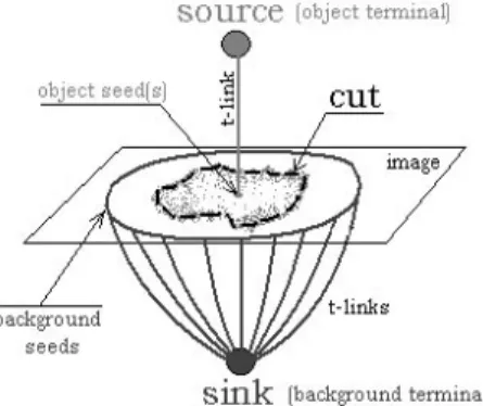
In this section we provide some technical details about our segmentation tech-nique. To segment an image we create a graph with nodes corresponding to pixels (voxels) of the image. There are two additional terminal nodes: an “object” ter-minal (a source) and a “background” terter-minal (a sink). The source is connected by edges to all nodes identified as object seeds and the sink is connected to all background seeds. For convenience, all edges from the terminals are referred to as t-links. We assign an infinite cost to all t-links between the seeds and the terminals.
Pairs of neighboring pixels (voxels) are connected by weighted edges that we calln-links(neighborhood links). Any kind of neighborhood system can be used. Costs of n-links can be based on local intensity gradient, Laplacian zero-crossing, gradient direction, and other criteria (e.g. [18]). The only technical restriction is that the edge costs should be non-negative. Our simplest implementation incorporates undirected n-links {p, q} between neighboring pixels pand q (see (a) below) with costw{p,q}=f(|Ip−Iq|) whereIpandIq are intensities at pixels pandqandf(x) =K·exp(−xσ22) is a non-negative decreasing function.
Such weights encourage segmentation boundaries in places with high intensity gradient. In some examples we also use directed links (p, q) and (q, p) between pixels pand q(see (b)). The weights can be defined asw(p,q)=max(0, f(|Ip− Iq|) +h·(Ip−Iq)) where the gradient direction is incorporated. A positive h forces dark pixels to stay inside the segmentation boundary and bright pixels to stay outside. A negativehwould achieve the opposite effect.
The general graph structure is now completely specified. Some examples are shown in Figure 2. We draw the segmentation boundary between the object and the background by finding the minimum cost cut on this graph. A cut is a subset of edges that separates the source from the sink. The cost of the cut is the sum of its edge costs1. Due to infinite cost of t-links to seeds, a minimum cut
1In case of directed edges the cost of the cut is the sum of severed edges (p, q) where
nodepis left in the part of the graph connected to the source andq is in the part connected to the sink.
is guaranteed to separate the object seeds from the background seeds. Note that locations with high intensity gradient correspond to cheap n-links. Thus, they are attractive choices for the optimal segmentation boundary. The minimum cut can be computed exactly in polynomial time using well known algorithms for two terminal graph cuts, e.g. max-flow [9] or push-relabel [11].
It is important that the algorithm efficiently adjusts the segmentation to in-corporate any additional seeds that the user might interactively add. We use a max flow algorithm to determine the minimum cut corresponding to the optimal segmentation. When a new seed is added to the image, the corresponding t-link is added to theresidualgraph that was left at the end of the previous cut compu-tation. Then, a new optimal cut can be efficiently obtained without recomputing the whole solution2. Deleting a seed from the image is equivalent to adding a t-link to the opposite terminal. Thus, it can also be efficiently implemented.
(a) Segmentation of a single object in a 2D image. A cut corresponds to a closed contour separating an object seed from background seeds.
(b) Segmentation of multiple objects in a 3D image. The cut separates the ob-ject seeds from the background seeds and creates two isolated object seg-ments.
Fig. 1.Examples of graphs for segmentation of 2D and 3D images.
3
Examples
In this section we consider a number of examples that illustrate how our method can be used to segment medical images. Section 3.1 shows the simplest 2D ex-periments and explains the main intuitions about our technique. Segmentation of multiple objects is discussed in Sections 3.2. 3D volume segmentation is ad-dressed in Section 3.3.
3.1 Single Object in 2D Images
In this section we show an example of the simplest application for our technique. The goal is to segment an object from the background in a given 2D image. We
assume that the object appears as one connected blob. The user places object seeds and background seeds to define areas that should be separated by the segmentation.
In Figure 2(a-d) we show the segmentation results for a 2D cardiac MR image. Our interface allows a user to enter seeds with a brush controlled through a mouse. The size of the brush can be changed. Throughout the paper we indicate object and background seeds by bright red and blue colors, respectively. The pixels that the algorithm assigned to the object segment are highlighted in red and background pixels appear bluish. In Figure 2(a) there is only one object segment. In fact, our algorithm is guaranteed to generate a single object segment when the object seeds form one connected group. The segmentation boundary defines a contour with the smallest cost among all contours separating the red (object) seeds from the blue (background) seeds. The computation time on a Pentium II, 333Mhz, for the segmentation of the 128×128 image shown in (a) is 50 milliseconds.
The example in Figure 2(a) shows that in a simple 2D setting our method can be used to extract a single closed contour which is what snakes, deformable templates, or shortest path search algorithms are used for. However, parts (b-d) of the same figure demonstrate the flexibility of our user interface combined with the graph cut segmentation. Our method provides a very simple and intuitive way to adjust the segmentation to the user liking. For example, in (a) the object segment covers only a blood pool. If the user wants to outline the epicardium, as shown in (b), it is enough to draw a few object seeds in the myocardium. Alternatively, if the user wants to get an accurate measurement of the endo-cardium as in (c), (s)he might have to add a few object seeds in the area of low contrast in the blood pool and a few background seeds in the myocardium. Our technique also allows the user to exclude internal parts of the object from the segmentation. For example, if the user wants to exclude papillary muscles from a volume measurement then (s)he can add background seeds inside these muscles as shown in (d). It should be noted that (b-d) are obtained directly from (a) by adding new seeds and the extra running time is negligible.
Figure 2(e) shows a segmented CT image of the liver. The original data is 512×512 pixels and the initial segmentation takes 1 to 2 seconds. Additional correcting seeds are processed in 100 to 200 milliseconds. This examples high-lights the use of directed n-links. When undirected n-links are used as in Figure 2(f), the segmentation boundary oscillates between neighboring edges that are very close together, always choosing the best edge. When directed n-links are used as in Figure 2(g), the boundary is forced to keep brighter pixels inside. Thus, the segmentation boundary coincides with the physical boundary of the organ. In general, the user can achieve any segmentation result that (s)he wants. If the results are not satisfactory in some part of the image, the user can add new object and background seeds providing additional clues where the segmentation was wrong, until all problems are corrected. The exact choice of seed position-ing is not relevant. Normally, movposition-ing object seeds within a region of “similar”
intensity inside one object segment cannot change the optimal segmentation3. It can also be shown that adding new object seeds inside the object segment will not change the resulting segmentation. Both properties are equally true for background seeds.
3.2 Multiple Objects
This section gives more general examples illustrating several important proper-ties of our algorithm. The goal is still to segment an object from the background. This time we assume that the image may contain several isolated objects of in-terest. For example, an MR image may contain ten blood vessels and a doctor may want to investigate two of them. The object seeds provide the necessary clues on what parts of the image are interesting to the user. There are no strict requirements on where the object seeds have to be placed as long as they are inside the object(s) of interest. Such flexibility is justified, in part, by the ability of the algorithm to efficiently incorporate the seeds added later on, when the initial segmentation results are not satisfactory. The object seeds can be placed sparingly and they do not necessarily have to be connected inside each isolated object. Potentially, the algorithm can create as many separate object segments as there are connected components of object seeds. Nonetheless, the isolated seeds (or components of seeds) located not too far from each other inside the same object are likely to be segmented out together. Figure 3(d) illustrates this property of our technique. Figure 3(d) also shows that seeds can be placed to achieve any desired segmentation. We segmented the left kidney as one object by placing a single object “seed” in the middle. We segmented the callices out in the right kidney by placing background seeds in them. The segmentation al-gorithm automatically decides which object (or background) seeds are grouped into one connected segment and which seeds are placed separately. Note that this property may be also useful in N dimensions when a user does not see how the objects of interest connect when placing the seeds.
The background seeds should provide the clues on what is notan object of interest. In many situations the pixels on the image boundary are a good choice for background seeds. If the objects of interest are bright, then background seeds can be spread out in the dark parts of the image. Note that background seeds are very useful when two similar objects touch in some area of the image and one of them is of interest while the other is not. In this case there is a chance that the two objects may be merged into a single segment. This can be avoided by placing a background seed in the undesired object which would force the segmentation to separate the two objects at their merge point. Also, when the segmentation merges two objects of interest that should be separated, the user can add a background seed in between to effectively separate the two objects. This property is illustrated in Figure 3(a-c). At first, in Figure 3(c), the segmentation process grouped the two vessels together. By adding a single
background seed right between the two vessels, as in Figure 3(b), the user forced the process to keep the two objects separated.
3.3 3D Volumes
One example of the general graph structure for a multi-object segmentation in 3D is shown in Figure 2(b). The 3D segmentation has the same properties that we discussed for 2D examples. The main difficulty in 3D is to create a convenient interface for entering seeds. In fact, the ability to scan through a pile of 2D slices was good enough for our purpose. The user can select a few representative slices and enter object and background seeds in these slices. Since all voxels are connected in a 3D graph the information on what parts of the 3D volume are of interest and what parts should be considered background will propagate appropriately. Moreover, upon the initial segmentation the user can scan through the segmented slices and enter correcting seeds in some of the slices where the results are not satisfactory.
Figure 4 shows an example in cardiac MR. We took images of a slice of the heart left ventricle at different time instances and stacked them up into a volume. We then placed seeds in one image in the middle of the volume to indicate that we were interested in the blood pool. The resulting segmentation was almost perfect. We just had to add a couple of background seeds in the first and last slice to fill a small notch in the myocardium. The system was able to also fill the notch in the neighboring slices by propagating the new seeds. This segmentation of 12 256×256 images was done in 5 seconds.
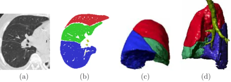
Figure 5 shows a segmentation that we obtained for 3D lung CT data. Each of the lobes and trachea were segmented separately. The segments we combined to obtain multi colored visualization.
4
Conclusions and Future Research
There are several important ideas that we are currently working on. First of all we can incorporate additional regional information by adding finite cost t-links to all non-seed pixels/voxels. Such t-links would connect a pixel to both the object and the background terminals. The costs can reflect how well the pixel’s intensity fits into available models of object and background, correspondingly. For example, such models can be represented by intensity histograms of seeded regions. These finite cost t-links are similar to what is used in [2]. Also, we can use approximation multi-way graph cut algorithms [2] to obtain multi-label segmentation. Such segmentation would be able to generate multi colored seg-mentation similar to what we show in Figure 5 without the need to segment each component independently.
We are also interested to try our segmentation technique on 4D data. To decrease the execution time and increase the memory efficiency of our software, especially for large 3D volumes and 4D datasets, we are considering representing the data using a quad-tree to group very similar pixels and associate groups to single nodes in the graph.
5
Acknowledgements
We would like to thank Bernhard Geiger for providing the 3D visualizations of the segmented volumes. Vladimir Kolmogorov helped us with some of the coding. Finally, discussions with Gareth Funka-Lea and Alok Gupta were very fruitfull.
References
1. A. A. Amini, T. E. Weymouth, and R. C. Jain. Using dynamic programming for solving variational problems in vision.IEEE Transactions on Pattern Analysis and Machine Intelligence, 12(9):855–867, September 1990.
2. Y. Boykov, O. Veksler, and R. Zabih. Markov random fields with efficient approxi-mations. InIEEE Conference on Computer Vision and Pattern Recognition, pages 648–655, 1998.
3. L. D. Cohen. On active contour models and ballons. Computer Vision, Graphics, and Image Processing: Image Understanding, 53(2):211–218, 1991.
4. L. D. Cohen and I. Cohen. Finite element methods for active contour models and ballons for 2-d and 3-d images. IEEE Transactions on Pattern Analysis and Machine Intelligence, 15(11):1131–1147, November 1993.
5. I. J. Cox, S. B. Rao, and Y. Zhong. ”Ratio regions”: A technique for image segmentation. In International Conference on Pattern Recognition, volume II, pages 557–564, 1996.
6. M.-P. Dubuisson-Jolly, C.-C. Liang, and A. Gupta. Optimal polyline tracking for artery motion compensation in coronary angiography. InInternational Conference on Computer Vision, pages 414–419, 1998.
7. A. X. Falc˜ao, J. K. Udupa, S. Samarasekera, and S. Sharma. User-steered image segmentation paradigms: Live wire and live lane. Graphical Models and Image Processing, 60:233–260, 1998.
8. M. Flickner, H. Sawhney, D. Pryor, and J. Lotspiech. Intelligent interactive image outlining using spline snakes. In Asilomar Conference on Signals, Systems, and Computers, volume 1, pages 731–735, 1994.
9. L. Ford and D. Fulkerson. Flows in Networks. Princeton University Press, 1962. 10. D. Geiger, A. Gupta, L. A. Costa, and J. Vlontzos. Dynamic programming for
detecting, tracking, and matching deformable contours. IEEE Transactions on Pattern Analysis and Machine Intelligence, 17(3):294–402, March 1995.
11. A. Goldberg and R. Tarjan. A new approach to the maximum flow problem. Journal of the Association for Computing Machinery, 35(4):921–940, October 1988. 12. D. Greig, B. Porteous, and A. Seheult. Exact maximum a posteriori estimation for binary images. Journal of the Royal Statistical Society, Series B, 51(2):271–279, 1989.
13. L. D. Griffin, A. C. F. Colchester, S. A. R¨oll, and C. S. Studholme. Hierarchical segmentation satisfying constraints. InBritish Machine Vision Conference, pages 135–144, 1994.
14. R. M. Haralick and L. G. Shapiro. Computer and Robot Vision. Addison-Wesley Publishing Company, 1992.
15. H. Ishikawa and D. Geiger. Segmentation by grouping junctions. In IEEE Con-ference on Computer Vision and Pattern Recognition, pages 125–131, 1998.
16. I. H. Jermyn and H. Ishikawa. Globally optimal regions and boundaries. In Inter-national Conference on Computer Vision, volume II, pages 904–910, 1999. 17. M. Kass, A. Witkin, and D. Terzolpoulos. Snakes: Active contour models.
Inter-national Journal of Computer Vision, 2:321–331, 1988.
18. E. N. Mortensen and W. A. Barrett. Interactive segmentation with intelligent scissors. Graphical Models and Image Processing, 60:349–384, 1998.
19. T. O’Donnell, M.-P. Dubuisson-Jolly, and A. Gupta. A cooperative framework for segmentation using 2D active contours and 3D hybrid models as applied to branching cylindrical structures. InInternational Conference on Computer Vision, pages 454–459, 1998.
20. L. J. Reese. Intelligent paint: Region-based interactive image segmentation. Mas-ter’s thesis, Brigham Young University, 1999.
21. J. Shi and J. Malik. Normalized cuts and image segmentation. InIEEE Conference on Computer Vision and Pattern Recognition, pages 731–737, 1997.
22. T. Vehkom¨aki, G. Gerig, and G. Sz´ekely. A user-guided tool for efficient segmen-tation of medical image data. InCVRMed-MRCAS, pages 685–694, 1997. 23. D. J. Williams and M. Shah. A fast algorithm for active contours and curvature
estimation.Computer Vision, Graphics, and Image Processing: Image Understand-ing, 55(1):14–26, 1992.
24. Z. Wu and R. Leahy. An optimal graph theoretic approach to data clustering: Theory and its application to image segmentation. IEEE Transactions on Pattern Analysis and Machine Intelligence, 15(11):1101–1113, November 1993.
25. A. Yuille and P. Hallinan. Deformable templates. In Andrew Blake and Alan Yuille, editors,Active Vision, pages 20–38. MIT Press, 1992.
26. S. C. Zhu and A. Yuille. Region competition: Unifying snakes, region growing, and Bayes/MDL for multiband image segmentation. IEEE Transactions on Pattern Analysis and Machine Intelligence, 18(9):884–900, September 1996.
Fig. 2. Single object segmentation. (a-d): Cardiac MRI. (e-g): Liver CT. Directed (f) and undirected (g) n-links.
Fig. 3. Segmentation of multiple objects. (a-c): Cardiac MRI. (d): Kidney CE-MR angiography.
Fig. 4.Volume segmentation of the blood pool in the heart left ventricle in MR.
(a) (b) (c) (d)
Fig. 5.Segmentation of the right lung in CT. (a): representative 2D slice of original 3D data. (b): segmentation results on the slice in (a). (c-d) 3D visualization of segmentation results.