Bayesian Learning in Social Networks

NBER WORKING PAPER SERIES

BAYESIAN LEARNING IN SOCIAL NETWORKS Daron Acemoglu Munther A. Dahleh Ilan Lobel Asuman Ozdaglar Working Paper 14040 http://www.nber.org/papers/w14040

NATIONAL BUREAU OF ECONOMIC RESEARCH 1050 Massachusetts Avenue

Cambridge, MA 02138 May 2008

We thank Lones Smith and Peter Sorensen for useful comments and suggestions. We gratefully acknowledge financial suppoert from AFOSR and the NSF. The views expressed herein are those of the author(s) and do not necessarily reflect the views of the National Bureau of Economic Research.

NBER working papers are circulated for discussion and comment purposes. They have not been peer-reviewed or been subject to the review by the NBER Board of Directors that accompanies official NBER publications.

© 2008 by Daron Acemoglu, Munther A. Dahleh, Ilan Lobel, and Asuman Ozdaglar. All rights reserved. Short sections of text, not to exceed two paragraphs, may be quoted without explicit permission provided that full credit, including © notice, is given to the source.

Bayesian Learning in Social Networks

Daron Acemoglu, Munther A. Dahleh, Ilan Lobel, and Asuman Ozdaglar NBER Working Paper No. 14040

May 2008

JEL No. C72,D83

ABSTRACT

We study the perfect Bayesian equilibrium of a model of learning over a general social network. Each individual receives a signal about the underlying state of the world, observes the past actions of a stochastically-generated neighborhood of individuals, and chooses one of two possible actions. The stochastic process generating the neighborhoods defines the network topology (social network). The special case where each individual observes all past actions has been widely studied in the literature. We characterize pure-strategy equilibria for arbitrary stochastic and deterministic social networks and characterize the conditions under which there will be asymptotic learning -- that is, the conditions under which, as the social network becomes large, individuals converge (in probability) to taking the right action. We show that when private beliefs are unbounded (meaning that the implied likelihood ratios are unbounded), there will be asymptotic learning as long as there is some minimal amount of "expansion in observations". Our main theorem shows that when the probability that each individual observes some other individual from the recent past converges to one as the social network becomes large, unbounded private beliefs are sufficient to ensure asymptotic learning. This theorem therefore establishes that, with unbounded private beliefs, there will be asymptotic learning an almost all reasonable social networks. We also show that for most network topologies, when private beliefs are bounded, there will not be asymptotic learning. In addition, in contrast to the special case where all past actions are observed, asymptotic learning is possible even with bounded beliefs in certain stochastic network topologies.

Daron Acemoglu Department of Economics MIT, E52-380B 50 Memorial Drive Cambridge, MA 02142-1347 and NBER [email protected] Munther A. Dahleh

Dept. of Electrical Engineering and Computer Science

Massachusetts Institute of Technology 77 Massachusetts Ave, 32D-734 Cambridge, MA 02139

[email protected]

Ilan Lobel

Operations Research Center

Massachusetts Institute of Technology 77 Massachusetts Ave, E40-130 Cambridge, MA 02139

[email protected] Asuman Ozdaglar

Dept of Electrical Engineering and Computer Science

Massachusetts Institute of Technology 77 Massachusetts Ave, E40-130 Cambridge, MA 02139

1

Introduction

How is dispersed and decentralized information held by a large number of individuals ag-gregated? Imagine a situation in which each of a large number of individuals has a noisy signal about an underlying state of the world. This state of the world might concern, among other things, earning opportunities in a certain occupation, the quality of a new product, the suitability of a particular political candidate for office or payoff-relevant ac-tions taken by the government. If signals are unbiased, the combination—aggregation— of the information of the individuals will be sufficient for the society to “learn” the true underlying state. The above question can be formulated as the investigation of what types of behaviors and communication structures will lead to this type of information aggregation.

Condorcet’s Jury Theorem provides a natural benchmark, where sincere (truthful) reporting of their information by each individual is sufficient for aggregation of informa-tion by a law of large numbers argument (Condorcet, 1788). Against this background, a number of papers, most notably Bikchandani, Hirshleifer and Welch (1992), Banerjee (1992) and Smith and Sorensen (2000), show how this type of aggregation might fail in the context of the (perfect) Bayesian equilibrium of a dynamic game: when individuals act sequentially, after observing the actions of all previous individuals (agents), many reasonable situations will lead to the wrong conclusion with positive probability.

An important modeling assumption in these papers is that each individual observes all past actions. In practice, individuals are situated in complex social networks, which provide their main source of information. For example, Granovetter (1973), Montgomery (1991), Munshi (2003) and Iaonnides and Loury (2004) document the importance of information obtained from the social network of an individual for employment outcomes. Besley and Case (1994), Foster and Rosenzweig (1995), Munshi (2004), and Udry and Conley (2001) show the importance of the information obtained from social networks for technology adoption. Jackson (2006, 2007) provide excellent surveys of the work on the importance of social networks in many diverse situations. In this paper, we address how the structure of social networks, which determines the information that individuals receive, affects equilibrium information aggregation.

We start with the canonical sequential learning problem, except that instead of full observation of past actions, we allow for a generalsocial network connecting individuals. More specifically, a large number of agents sequentially choose between two actions. An underlying state determines the payoffs of these two actions. Each agent receives a signal on which of these two actions yields a higher payoff. Preferences of all agents are aligned in the sense that, given the underlying state of the world, they all prefer the same action. The game is characterized by two features: (i) the signal structure, which determines how informative the signals received by the individuals are; (ii) the social network structure, which determines the observations of each individual in the game. We model the social network structure as a stochastic process that determines each individual’s neighborhood. Each individual only observes the (past) actions of agents in his neighborhood. Motivated by the social network interpretation, throughout it is assumed that each individual knows the identity of the agents in his neighborhood (e.g., he can distinguish whether the action observed is by a friend or neighbor or by some

outside party). Nevertheless, the realized neighborhood of each individual as well as his private signal are private information.

We also refer to the stochastic process generating neighborhoods as the network topology of this social network. For some of our results, it will be useful to distinguish between deterministic and stochastic network topologies. With deterministic network topologies, there is no uncertainty concerning the neighborhood of each individual and these neighborhoods are common knowledge. With stochastic network topologies, there is uncertainty about these neighborhoods.

The environment most commonly studied in the previous literature is the full obser-vation network topology, which is the special case where all past actions are observed. Another deterministic special case is the network topology where each individual ob-serves the actions of the most recent M ≥1 individuals. Other relevant social networks include stochastic topologies in which each individual observes a random subset of past actions, as well as those in which, with a high probability, each individual observes the actions of some “influential” group of agents, who may be thought of as “leaders” or the media.

We provide a systematic characterization of the conditions under which there will be equilibrium information aggregation in social networks. We say that there isinformation aggregation or equivalently asymptotic learning, when, in the limit as the size of the social network becomes arbitrarily large, individual actions converge (in probability) to the action that yields the higher payoff. We say that asymptotic learning fails if, as the social network becomes large, the correct action is not chosen (or more formally, the lim inf of the probability that the right action is chosen is strictly less than 1).

Two concepts turn out to be crucial in the study of information aggregation in social networks. The first is whether thelikelihood ratio implied by individual signals is always finite and bounded away from 0.1 _{Smith and Sorensen (2000) refer to beliefs that satisfy} this property as bounded (private) beliefs. With bounded beliefs, there is a maximum amount of information in any individual signal. In contrast, when there exist signals with arbitrarily high and low likelihood ratios,(private) beliefs are unbounded. Whether bounded or unbounded beliefs provide a better approximation to reality is partly an interpretational and partly an empirical question. Smith and Sorensen’s main result is that when each individual observes all past actions and private beliefs are unbounded, information will be aggregated and the correct action will be chosen asymptotically. In contrast, the results in Bikchandani, Hirshleifer and Welch (1992), Banerjee (1992) and Smith and Sorensen (2000) indicate that with bounded beliefs, there will not be asymp-totic learning (or information aggregation). Instead, as emphasized by Bikchandani, Hirshleifer and Welch (1992) and Banerjee (1992), there will be “herding” or “infor-mational cascades,” where individuals copy past actions and/or completely ignore their own signals.

The second key concept is that of a network topology with expanding observations. To describe this concept, let us first introduce another notion: a finite group of agents is

excessively influential if there exists an infinite number of agents who, with probability 1_{The likelihood ratio is the ratio of the probabilities or the densities of a signal in one state relative}

uniformly bounded away from 0, observe only the actions of a subset of this group. For example, a group is excessively influential if it is the source of all information (except individual signals) for an infinitely large component of the social network. If there exists an excessively influential group of individuals, then the social network hasnonexpanding observations, and conversely, if there exists no excessively influential group, the network hasexpanding observations. This definition implies that most reasonable social networks have expanding observations, and in particular, a minimum amount of “arrival of new information ” in the social network is sufficient for the expanding observations property.2 For example, the environment studied in most of the previous work in this area, where all past actions are observed, has expanding observations. Similarly, a social network in which each individual observes one uniformly drawn individual from those who have taken decisions in the past or a network in which each individual observes his immedi-ate neighbor all feature expanding observations. Note also that a social network with expanding observations need not beconnected. For example, the network in which even-numbered [odd-even-numbered] individuals only observe the past actions of even-even-numbered [odd-numbered] individuals has expanding observations, but isnotconnected. A simple, but typical, example of a network with nonexpanding observations is the one in which all future individuals only observe the actions of the first K <∞ agents.

Our main results in this paper are presented in four theorems.

1. Theorem 1 shows that there is no asymptotic learning in networks with nonexpand-ing observations. This result is not surprisnonexpand-ing, since information aggregation is not possible when the set of observations on which (an infinite subset of) individuals can build their decisions remains limited forever.

2. Our most substantive result, Theorem 2, shows that when (private) beliefs are un-bounded and the network topology is expanding, there will be asymptotic learning. This is a very strong result (particularly if we consider unbounded beliefs to be a better approximation to reality than bounded beliefs), since almost all reasonable social networks have the expanding observations property. This theorem, for ex-ample, implies that when some individuals, such as “informational leaders,” are overrepresented in the neighborhoods of future agents (and are thus “influential,” though not excessively so), learning may slow down, but asymptotic learning will still obtain as long as private beliefs are unbounded.

The idea of the proof of Theorem 2 is as follows. We first establish a strong improvement principle under unbounded beliefs, whereby in a network where each individual has a single agent in his neighborhood, he can receive a strictly higher payoff than this agent and this improvement remains bounded away from zero as long as asymptotic learning has not been achieved. We then show that the same insight applies when individuals stochastically observe one or multiple agents (in particular, with multiple agents, the improvement is no less than the case in which the individual observes a single agent from the past). Finally, the property that the 2_{Here, “arrival of new information” refers to the property that the probability of each individual}

observing the action of some individual from the recent past converges to one as the social network becomes arbitrarily large.

network topology has expanding observations is sufficient for these improvements to accumulate to asymptotic learning.

3. Theorem 3 presents a partial converse to Theorem 2. It shows that for the most common deterministic and stochastic networks, bounded private beliefs are in-compatible with asymptotic learning. It therefore generalizes existing results on asymptotic learning, for example, those in Bikchandani, Hirshleifer and Welch (1992), Banerjee (1992), and Smith and Sorensen (2000) to general networks. 4. Our final main result, Theorem 4, establishes that asymptotic learning is possible

with bounded private beliefs for certain stochastic network topologies. In these cases, there is sufficient arrival of new information (incorporated into the “social belief”) because some agents make decisions on the basis of limited observations. As a consequence, even bounded private beliefs may aggregate and lead to asymp-totic learning. This finding is particularly important, since it shows how moving away from simple network structures has major implications for equilibrium learn-ing dynamics.

The rest of the paper is organized as follows. The next section discusses the re-lated literature and clarifies the contribution of our paper. Section 3 introduces the model. Section 4 formally introduces the concepts of bounded and unbounded beliefs, and network topologies with expanding and nonexpanding observations. This section then presents our main results, Theorems 1-4, and discusses some of their implications (as well as presenting a number of corollaries to facilitate interpretation). The rest of the paper characterizes the (pure-strategy) perfect Bayesian equilibria of the model pre-sented in Section 3 and provides proofs of these theorems. Section 5 presents a number of important results on the characterization of pure-strategy equilibria. Section 6 occu-pies the bulk of the paper and provides a detailed proof of Theorem 2, which involves the statement and proof of several lemmas. Section 7 provides a proof of Theorem 3, while Section 8 shows how asymptotic learning is possible with bounded private beliefs. Section 9 concludes. Appendices A and B contain proofs omitted from the main text, including the proof of Theorem 1.

2

Related Literature

The literature on social learning is vast. Roughly speaking, the literature can be sep-arated according to two criteria: whether learning is Bayesian or myopic, and whether individuals learn from communication of exact signals or from the payoffs of others, or simply from observing others’ actions. Typically, Bayesian models focus on learning from past actions, while most, but not all, myopic learning models focus on learning from communication.

Bikchandani, Hirshleifer and Welch (1992) and Banerjee (1992) started the litera-ture on learning in situations in which individuals are Bayesian and observe past actions. Smith and Sorensen (2000) provide the most comprehensive and complete analysis of

this environment. Their results and the importance of the concepts of bounded and un-bounded beliefs, which they introduced, have already been discussed in the introduction and will play an important role in our analysis in the rest of the paper. Other important contributions in this area include, among others, Welch (1992), Lee (1993), Chamley and Gale (1994), and Vives (1997). An excellent general discussion is contained in Bikchan-dani, Hirshleifer and Welch (1998). These papers typically focus on the special case of full observation network topology in terms of our general model.

The two papers most closely related to ours are Banerjee and Fudenberg (2004) and Smith and Sorensen (1998). Both of these papers study social learning with sampling of past actions. In Banerjee and Fudenberg, there is a continuum of agents and the focus is on proportional sampling (whereby individuals observe a “representative” sample of the overall population). They establish that asymptotic learning is achieved under mild assumptions as long as the sample size is no smaller than two. The existence of a continuum of agents is important for this result since it ensures that the fraction of individuals with different posteriors evolves deterministically. Smith and Sorensen, on the other hand, consider a related model with a countable number of agents. In their model, as in ours, the evolution of beliefs is stochastic. Smith and Sorensen provide conditions under which asymptotic learning takes place.

A crucial difference between Banerjee and Fudenberg and Smith and Sorensen, on the one hand, and our work, on the other, is the information structure. These papers assume that “samples are unordered” in the sense that individuals do not know the identity of the agents they have observed. In contrast, as mentioned above, our setup is motivated by a social network and assumes that individuals have stochastic neigh-borhoods, but know the identity of the agents in their realized neighborhood. We view this as a better approximation to learning in social networks. In addition to its descrip-tive realism, this assumption leads to a sharper characterization of the conditions under which asymptotic learning occurs. For example, in Smith and Sorensen’s environment, asymptotic learning fails whenever an individual is “oversampled,” in the sense of being overrepresented in the samples of future agents. In contrast, in our environment, asymp-totic learning occurs when the network topology features expanding observations (and private beliefs are unbounded). Expanding observations is a much weaker requirement than “non-oversampling.” For example, when each individual observes agent 1 and a randomly chosen agent from his predecessors, the network topology satisfies expanding observations, but there is oversampling.3

Other recent work on social learning includes Celen and Kariv (2004) who study Bayesian learning when each individual observes his immediate predecessor, Gale and Kariv (2003) who generalize the payoff equalization result of Bala and Goyal (1998) in connected social networks (discussed below) to Bayesian learning, and Callander and Horner (2006), who show that it may be optimal to follow the actions of agents that deviate from past average behavior.

The second branch of the literature focuses on non-Bayesian learning, typically with agents using some reasonable rules of thumb. This literature considers both learning from 3_{This also implies that, in the terminology of Bala and Goyal, a “royal family” precludes learning}

past actions and from payoffs (or directly from beliefs). Early papers in this literature include Ellison and Fudenberg (1993, 1995), which show how rule-of-thumb learning can converge to the true underlying state in some simple environments. The papers most closely related to our work in this genre are Bala and Goyal (1998, 2001), DeMarzo, Vayanos and Zwiebel (2003) and Golub and Jackson (2007). These papers study non-Bayesian learning over an arbitrary, connected social network. Bala and Goyal (1998) establish the important and intuitive payoff equalization result that, asymptotically, each individual must receive a payoff equal to that of an arbitrary individual in his “social network,” since otherwise he could copy the behavior of this other individual. Our paper can be viewed as extending Bala and Goyal’s results to a situation with Bayesian learning. A similar “imitation” intuition plays an important role in our proof of asymptotic learning with unbounded beliefs and unbounded observations.

DeMarzo, Vayanos and Zwiebel and Golub and Jackson also study similar environ-ments and derive consensus-type results, whereby individuals in the connected compo-nents of the social network will converge to similar beliefs. They provide characterization results on which individuals in the social network will be influential and investigate the likelihood that the consensus opinion will coincide with the true underlying state. Golub and Jackson, in particular, show that social networks where some individuals are “influ-ential” in the sense of being connected to a large number of people make learning more difficult or impossible. A similar result is also established in Bala and Goyal, where they show that the presence of a royal family, i.e., a small set of individuals observed by everyone, precludes learning. This both complements and contrasts with our results. In our environment, an excessively influential group of individuals prevents learning, but influential agents in Golub and Jackson’s sense or Bala and Goyal’s royal family are not excessively influential and still allow asymptotic learning. This is because with Bayesian updating over a social network, individuals recognize who the oversampled individuals or the royal family are and accordingly adjust the weight they give to their action/information.

The literature on the information aggregation role of elections is also related, since it revisits the original context of Condorcet’s Jury Theorem. This literature includes, among others, the papers by Austen-Smith and Banks (1996), Feddersen and Pesendorfer (1996, 1997), McLennan (1998), Myerson (1998, 2000), and Young (1988). Most of these papers investigate whether dispersed information will be accurately aggregated in large elections. Although the focus on information aggregation is common, the set of issues and the methods of analysis are very different, particularly since, in these models, there are no sequential decisions.

Finally, there is also a literature in engineering, which studies related problems, especially motivated by aggregation of information collected by decentralized sensors. These include Cover (1969), Papastavrou and Athans (1990), Lorenz, Marciniszyn and, Steger (2007), and Tay, Tsitsiklis and Win (2007). The work by Papastavrou and Athans contains a result that is equivalent to the characterization of asymptotic learning with the observation of the immediate neighbor.

3

Model

A countably infinite number of agents (individuals), indexed by n ∈ N, sequentially make a single decision each. The payoff of agent n depends on an underlying state of the world θ and his decision. To simplify the notation and the exposition, we assume that both the underlying state and decisions are binary. In particular, the decision of agent n is denoted by xn ∈ {0,1} and the underlying state is θ ∈ {0,1}. The payoff of

agent n is

un(xn, θ) =

½

1 if xn=θ

0 ifxn 6=θ.

Again to simplify notation, we assume that both values of the underlying state are equally likely, so that P(θ = 0) =P(θ= 1) = 1/2.

The state θ is unknown. Each agent n ∈ N forms beliefs about this state from a

private signalsn∈S (whereS is a metric space or simply a Euclidean space) and from

his observation of the actions of other agents. Conditional on the state of the world θ, the signals are independently generated according to a probability measureFθ. We refer

to the pair of measures (F0,F1) as the signal structureof the model. We assume thatF0 and F1 are absolutely continuous with respect to each other, which immediately implies that no signal is fully revealing about the underlying state. We also assume thatF0 and F1 are not identical, so that some signals are informative. These two assumptions on the signal structure are maintained throughout the paper and will not be stated in the theorems explicitly.

In contrast to much of the literature on social learning, we assume that agents do not necessarily observe all previous actions. Instead, they observe the actions of other agents according to the structure of thesocial network. To introduce the notion of a social network, let us first define a neighborhood. Each agent n observes the decisions of the agents in his (stochastically-generated) neighborhood, denoted by B(n).4 _{Since agents} can only observe actions taken previously, B(n)⊆ {1,2, ..., n−1}. Each neighborhood B(n) is generated according to an arbitrary probability distribution Qn over the set of

all subsets of {1,2, ..., n−1}. We impose no special assumptions on the sequence of distributions {Qn}n∈N except that the draws from each Qn are independent from each

other for alln and from the realizations of private signals. The sequence {Qn}n∈N is the

network topology of the social network formed by the agents. The network topology is common knowledge, whereas the realized neighborhood B(n) and the private signal sn

are the private information of agentn. We say that{Qn}n∈N is a deterministicnetwork topology if the probability distributionQn is a degenerate (Dirac) distribution for all n.

Otherwise, that is, if{Qn}for somenis nondegenerate,{Qn}n∈Nis astochasticnetwork topology.

A social network consists of a network topology {Qn}n∈N and a signal structure (F0,F1).

Example 1 Here are some examples of network topologies.

4_Ifn0 _{∈B(n), then agentnnot only observes the action of n}0_{, but also knows the identity of this}

7 4 1 3 5 6 2 STATE

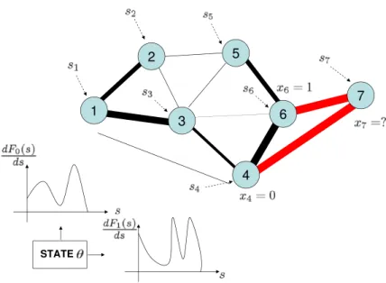
Figure 1: The figure illustrates the world from the perspective of agent 7. Agent 7 knows her private signal s7, her realized neighborhood, B(7) ={4,6}and the decisions of agents 4 and 6, x4 and x6. She also knows the probabilistic model {Qn}n<7 for neighborhoods of all agents n <7.

1. If {Qn}n∈N assigns probability 1 to neighborhood {1,2..., n−1} for each n ∈ N, then the network topology is identical to the canonical one studied in the previous literature where each agent observes all previous actions (e.g., Banerjee (1992), Bikchandani, Hirshleifer and Welch (1992), Smith and Sorensen (2000)).

2. If {Qn}n∈N assigns probability 1/(n −1) to each one of the subsets of size 1 of

{1,2..., n−1}for eachn ∈N, then we have a network topology of random sampling of one agent from the past.

3. If {Qn}n∈N assigns probability 1 to neighborhood {n−1} for each n ∈ N, then we have a network topology where each individual only observes his immediate neighbor (also considered in a different context in the engineering literature by Papastavrou and Athans (1990)).

4. If {Qn}n∈N assigns probability 1 to neighborhoods that are subsets of {1,2, ..., K} for each n ∈N for some K ∈N. In this case, all agents observe the actions of at most K agents.

5. Figure 1 depicts an arbitrary stochastic topology until agent 7. The thickness of the lines represents the probability with which a particular agent will observe the action of the corresponding preceding agent.

Given the description above, it is evident that the information set In of agent n is

is,

In ={sn, B(n), xk for all k ∈B(n)}. (1)

The set of all possible information sets of agent n is denoted by In. A strategy for individual n is a mapping σn : In → {0,1} that selects a decision for each possible

information set. A strategy profile is a sequence of strategies σ={σn}n∈N. We use the standard notation σ−n = {σ1, . . . , σn−1, σn+1, . . .} to denote the strategies of all agents

other than n and also (σn, σ−n) for any n to denote the strategy profile σ. Given a

strategy profile σ, the sequence of decisions {xn}n∈N is a stochastic process and we denote the measure generated by this stochastic process byPσ.

Definition 1 A strategy profile σ∗ _{is a pure-strategy Perfect Bayesian Equilibrium}

of this game of social learning if for each n ∈ N, σ∗

n maximizes the expected payoff of agent n given the strategies of other agents σ∗

−n.

In the rest of the paper, we focus on pure-strategy Perfect Bayesian Equilibria, and simply refer to this as “equilibrium” (without the pure-strategy and the Perfect Bayesian qualifiers).

Given a strategy profileσ, the expected payoff of agent n from actionxn=σn(In) is

simply Pσ(xn =θ | In). Therefore, for any equilibrium σ∗, we have

σ∗

n(In)∈arg max y∈{0,1}

P(y,σ∗

−n)(y =θ | In). (2) We denote the set of equilibria (pure-strategy Perfect Bayesian Equilibria) of the game by Σ∗_{. It is clear that Σ}∗ _{is nonempty. Given the sequence of strategies {σ}∗

1, . . . , σn∗−1}, the maximization problem in (2) has a solution for each agent n and each In ∈ In.

Proceeding inductively, and choosing either one of the actions in case of indifference determines an equilibrium. We note the existence of equilibrium here.

Proposition 1 There exists a pure-strategy Perfect Bayesian Equilibrium.

Our main focus is whether equilibrium behavior will lead to information aggregation. This is captured by the notion of asymptotic learning, which is introduced next.

Definition 2 Given a signal structure(F0,F1)and a network topology {Qn}n∈N, we say

thatasymptotic learning occurs in equilibrium σ ifxnconverges toθin probability (according to measure Pσ), that is,

lim

n→∞Pσ(xn =θ) = 1.

Notice that asymptotic learning requires that the probability of taking the correct action converges to 1. Therefore, asymptotic learning will fail when, as the network becomes large, the limit inferior of the probability of all individuals taking the correct action is strictly less than 1.

Our goal in this paper is to characterize conditions on social networks—on signal structures and network topologies—that ensure asymptotic learning.

4

Main Results

In this section, we present our main results on asymptotic learning, in particular, Theo-rems 1-4, and we discuss some of the implications of these theoTheo-rems. The proofs of the results stated in this section are provided in the rest of the paper.

We start by introducing the key properties of network topologies and signal struc-tures that impact asymptotic learning. Intuitively, for asymptotic learning to occur, the information that each agent receives from other agents should not be confined to a bounded subset of agents. This property is established in the following definition. For this definition and throughout the paper, if the setB(n) is empty, we set maxb∈B(n)b= 0. Definition 3 The network topology has expanding observations if for all K ∈ N, we have lim n→∞Qn µ max b∈B(n)b < K ¶ = 0.

If the network topology does not satisfy this property, then we say it hasnonexpanding observations.

Recall that the neighborhood of agentnis a random variableB(n) (with values in the set of subsets of{1,2, ..., n−1}) and distributed according toQn. Therefore, maxb∈B(n)b is a random variable that takes values in {0,1, ..., n−1}. The expanding observations condition can be restated as the sequence of random variables{maxb∈B(n)b}n∈N converg-ing to infinity in probability. Similarly, it follows from the precedconverg-ing definition that the network topology has nonexpanding observations if and only if there exists someK ∈N and some scalar ² >0 such that

lim sup n→∞ Qn µ max b∈B(n)b < K ¶ ≥².

An alternative restatement of this definition might clarify its meaning. Let us refer to a finite set of individuals C as excessively influential if there exists a subsequence of agents who, with probability uniformly bounded away from zero, observe the actions of a subset of C. Then, the network topology has nonexpanding observations if and only if there exists an excessively influential group of agents. Note also that if there is a minimum amount of arrival of new information in the network, so that the probability of an individual observing some other individual from the recent past goes to one as the network becomes large, then the network topology will feature expanding observations. This discussion therefore highlights that the requirement that a network topology has expanding observations is quite mild and most social networks satisfy this requirement. When the topology has nonexpanding observations, there is a subsequence of agents that draws information from the first K decisions with positive probability (uniformly bounded away from 0). It is then intuitive that network topologies with nonexpanding observations will preclude asymptotic learning. Our first theorem states this result. Though intuitive, the proof of this result is somewhat long and not essential for the rest of the argument and is thus provided in Appendix A.

Theorem 1 Assume that the network topology{Qn}n∈Nhas nonexpanding observations.

Then, there exists no equilibrium σ ∈Σ∗ _{with asymptotic learning.}

This theorem states the intuitive result that with nonexpanding observations, asymp-totic learning will fail. This result is not surprising, since asympasymp-totic learning requires theaggregation of the information of different individuals. But a network topology with nonexpanding observations does not allow such aggregation. Intuitively, nonexpanding observations, or equivalently the existence of an excessively influential group of agents, imply that infinitely many individuals will observe finitely many actions with positive probability and this will not enable them to aggregate the dispersed information collec-tively held by the entire social network.

The main question is then whether, once we exclude network topologies with nonex-panding observations, what other conditions need to be imposed to ensure asymptotic learning. To answer this question and state our main theorem, we need to introduce one more notion. Following Smith and Sorensen (2000), we define private beliefsas the posterior that the true state is θ = 1 given individual signal sn. We will see below

that private beliefs will play a key role in the characterization of equilibrium behavior. For now, let dF0/dF1 denote the Radon-Nikodym derivative of the measures F0 and F1 (recall that these are absolutely continuous with respect to each other). If F0 and F1 have densities, then for each j ∈ {0,1}, dFj can be replaced by the density of Fj. If

both measures have atoms at somes ∈S, then dF0/dF1(s) = F0(s)/F1(s).

Definition 4 The signal structure has bounded private beliefs if there exists some

0< m, M <∞ such that the Radon-Nikodym derivative dF0/dF1 satisfies

m < dF0 dF1

(s)< M,

for almost all s ∈S under measure (F0 +F1)/2. The signal structure has unbounded private beliefsif for anyS0 _{contained inSwith probability 1 under measure(F}

0+F1)/2, we have inf s∈S0 dF0 dF1 (s) = 0, and sup s∈S0 dF0 dF1 (s) = ∞.

Bounded private beliefs imply that there is a maximum amount of information that an individual can derive from his private signal. Conversely, unbounded private beliefs correspond to a situation where an agent can receive an arbitrarily strong signal about the underlying state (see Section 5.2 for a more detailed discussion of this property). Smith and Sorensen (2000) show that, in the special case of full observation network topology, there will be asymptotic learning if and only if private beliefs are unbounded. The following theorem shows that for general network topologies, unbounded pri-vate beliefs play a similar role. In particular, unbounded pripri-vate beliefs and expanding observations are sufficient for asymptotic learning in all equilibria.

Theorem 2 Assume that the signal structure(F0,F1)has unbounded private beliefs and

the network topology {Qn}n∈N has expanding observations. Then, asymptotic learning

The proof of this theorem, which is provided in Section 6, takes up a large part of the remainder of this paper. However, many of its implications can be discussed before presenting a detailed proof.

Theorem 2 is quite a striking result. It implies that unbounded private beliefs are sufficient for asymptotic learning for most (but not all) network topologies. In particu-lar, the condition that the network topology has expanding observations is fairly mild and only requires a minimum amount of arrival of recent information to the network. Social networks in which each individual observes all past actions, those in which each observes just his neighbor, and those in which each individual observes M ≥ 1 agents independently and uniformly drawn from his predecessors are all examples of network topologies with expanding observations. Theorem 2 therefore implies that unbounded private beliefs are sufficient to guarantee asymptotic learning in social networks with these properties and many others.

Nevertheless, there are interesting network topologies where asymptotic learning does not occur even with unbounded private signals. The following corollary to Theorems 1 and 2 shows that for an interesting class of stochastic network topologies, there is a critical topology at which there is a phase transition—that is, for all network topologies with greater expansion of observations than this critical topology, there will be asymp-totic learning and for all topologies with less expansion, asympasymp-totic learning will fail. The proof of this corollary is also provided in Section 6.

Corollary 1 Assume that the signal structure (F0,F1) has unbounded private beliefs.

Assume also that the network topology is given by {Qn}n∈N such that

Qn(m∈B(n)) =

A

(n−1)C for all n and all m < n,

where, given n, the draws for m, m0 _{< n are independent and A and C are positive}

constants. If C < 1 then asymptotic learning occurs in all equilibria. If C ≥ 1, then asymptotic learning does not occur in any equilibrium.

Given the class of network topologies in this corollary, C < 1 implies that as the network becomes large, there will be sufficient expansion of observations. In contrast, for C≥1, stochastic process Qn does not place enough probability on observing recent

actions and the network topology is nonexpanding. Consequently, Theorem 1 applies and there is no asymptotic learning.

To highlight the implications of Theorems 1 and 2 for deterministic network topolo-gies, let us introduce the following definition.

Definition 5 Assume that the network topology is deterministic. Then, we say a finite sequence of agentsπ is an information pathof agentn if for eachi, πi ∈B(πi+1) and

the last element of π is n. Let π(n) be an information path of agent n that has maximal length. Then, we let L(n) denote the number of elements in π(n) and call it agent n’s information depth.

Intuitively, the concepts of information path and information depth capture the intuitive notion of how long the “trail” of the information in the neighborhood of an

individual is. For example, if each individual observes only his immediate neighbor (i.e., B(n) = {n−1} with probability one), each will have a small neighborhood, but the information depth of a high-indexed individual will be high (or the “trail” will be long), because the immediate neighbor’s action will contain information about the signals of all previous individuals. The next corollary shows that with deterministic network topologies, asymptotic learning will occur if only if the information depth (or the trail of the information) increases without bound as the network becomes larger.

Corollary 2 Assume that the signal structure (F0,F1) has unbounded private beliefs. Assume that the network topology is deterministic. Then, asymptotic learning occurs for all equilibria if the sequence of information depths {L(n)}n∈N goes to infinity. If the

sequence {L(n)}n∈N does not go to infinity, then asymptotic learning does not occur in

any equilibrium.

In the full observation network topology, bounded beliefs imply lack of asymptotic learning. One might thus expect a converse to Theorem 2, whereby asymptotic learning fails whenever signals are bounded. Under general network topologies, learning dynam-ics turn out to be more interesting and richer. The next theorem provides a partial converse to Theorem 2 and shows that for a wide range of deterministic and stochastic network topologies, bounded beliefs imply no asymptotic learning. However, somewhat surprisingly, Theorem 4 will show that the same is not true with more general stochastic network topologies.

Theorem 3 Assume that the signal structure (F0,F1) has bounded private beliefs. If

the network topology {Qn}n∈N satisfies one of the following conditions,

(a) B(n) = {1, . . . , n−1} for all n, (b) |B(n)| ≤1 for all n, or

(c) there exists some constant M such that |B(n)| ≤M for all n and

lim

n→∞ bmax∈B(n)b=∞ with probability 1,

then, asymptotic learning does not occur in any equilibrium σ∈Σ∗_.

This theorem implies that in most common deterministic and stochastic network topologies, bounded private beliefs imply lack of asymptotic learning. The proof of Theorem 3 is presented in Section 7. Although Part (a) of this theorem is already proved by Smith and Sorensen (2000), we provide an alternative proof that highlights the importance of the concepts emphasized here.

The following corollary, which is also proved in Section 7, illustrates the implica-tions of Theorem 3. It shows that, when private beliefs are bounded, there will be no asymptotic learning (in any equilibrium) in stochastic networks with random sampling. Corollary 3 Assume that the signal structure (F0,F1) has bounded private beliefs. As-sume that each agentnsamplesM agents uniformly and independently among {1, ..., n−

1}, for some M ≥ 1. Then, asymptotic learning does not occur in any equilibrium

We next show that with general stochastic topologies asymptotic learning is possible. Let us first define the notion of anonpersuasive neighborhood.

Definition 6 A finite set B ⊂ N is a nonpersuasive neighborhood in equilibrium

σ∈Σ∗ _if

Pσ(θ = 1|xk =yk for all k ∈B)∈

¡

β, β¢

for any set of values yk ∈ {0,1} for each k. We denote the set of all nonpersuasive neighborhoods by Uσ.

A neighborhood B is nonpersuasive in equilibrium σ ∈Σ∗ _{if for any set of decisions}

that agent n observes, his behavior may still depend on his private signal. A nonper-suasive neighborhood is defined with respect to a particular equilibrium. However, it is straightforward to see thatB =∅, i.e., the empty neighborhood, is nonpersuasive in any equilibrium. Moreover the setB ={1}is nonpersuasive as long asPσ(θ= 1|x1 = 1)< β and Pσ(θ = 1|x1 = 0) > β. It can be verified that this condition is equivalent to

G1(1/2)<min ½µ β 1−β ¶ G0(1/2), µ β 1−β ¶ G0(1/2) + 1−2β 1−β ¾ .

Our main theorem for learning with bounded beliefs, which we state next, provides a class of stochastic social networks where asymptotic learning takes place for any signal structure. The proof of this theorem is presented in Section 6.

Theorem 4 Let (F0,F1) be an arbitrary signal structure. Let M be a positive integer

and let C1, ..., CM be sets such that Ci ∈ Uσ for all i = 1, . . . , M for some equilibrium

σ ∈Σ∗_{. For each i= 1, . . . , M, let {r}

i(n)} be a sequence of non-negative numbers such that lim n→∞ M X i=1 ri(n) = 0 and ∞ X n=1 M X i=1 ri(n) = ∞, (3) with PM_i=1ri(n)≤1 for all n and ri(n) = 0 for all n ≤ maxb∈Cib. Assume the network

topology satisfies

B(n) =

½

Ci, with probability ri(n) for each i from 1 to M, {1,2, ..., n−1}, with probability 1−PM_i=1ri(n).

Then, asymptotic learning occurs in equilibrium σ.

Clearly, this theorem could have been stated with Ci =∅ for all i= 1, . . . , m, which

would correspond to agentn making a decision without observing anybody else’s action with some probability r(n) = PM_i=1ri(n)≤1.

This is a rather surprising result, particularly in view of existing results in the liter-ature, which generate herds and information cascades (and no learning) with bounded beliefs. This theorem indicates that learning dynamics become significantly richer when we consider general social networks. In particular, certain stochastic network topologies enable a significant amount of new information to arrive into the network, because some

agents make decisions with limited information (nonpersuasive neighborhoods). As a result, the relevant information can be aggregated in equilibrium, leading to individuals’ decisions eventually converging to the right action (in probability).

It is important to emphasize the difference between this result and that in Sgroi (2002), which shows that a social planner can ensure some degree of information ag-gregation by forcing a subsequence of agents to make decisions without observing past actions. With the same reasoning, one might conjecture that asymptotic learning may occur if a particular subsequence of agents, such as that indexed by prime numbers, has empty neighborhoods. However, there will not be asymptotic learning in this determin-istic topology since lim infn→∞Pσ(xn =θ) <1. For the result that there is asymptotic

learning (i.e., lim infn→∞Pσ(xn = θ) = 1) in Theorem 4, the feature that the network

topology is stochastic is essential.

5

Equilibrium Strategies

In this section, we provide a characterization of equilibrium strategies. We show that equilibrium decision rules of individuals can be decomposed into two parts, one that only depends on an individual’s private signal, and the other that is a function of the observations of past actions. We also show why a full characterization of individual decisions is nontrivial and motivate an alternative proof technique, relying on developing bounds on improvements in the probability of the correct decisions, that will be used in the rest of our analysis.

5.1

Characterization of Individual Decisions

Our first lemma shows that individual decisions can be characterized as a function of the sum of two posteriors. These posteriors play an important role in our analysis. We will refer to these posteriors as the individual’s private belief and the social belief. Lemma 1 Let σ∈Σ∗ _{be an equilibrium of the game. Let I}

n ∈ In be an information set of agent n. Then, the decision of agent n, xn=σ(In), satisfies

xn = ½ 1, if Pσ(θ = 1 | sn) +Pσ ¡ θ = 1 | B(n), xk, k ∈B(n) ¢ >1, 0, if Pσ(θ = 1 | sn) +Pσ ¡ θ = 1 | B(n), xk, k ∈B(n) ¢ <1, and xn∈ {0,1} otherwise.

Proof. See Appendix B.

The lemma above establishes an additive decomposition in the equilibrium decision rule between the information obtained from the private signal of the individual and from the observations of others’ actions (in his neighborhood). The next definition formally distinguishes between the two components of an individual’s information.

Definition 7 We refer to the probability Pσ(θ= 1 | sn) as the private belief of agent

n, and the probability

Pσ

¡

θ = 1 ¯¯ B(n), xk for all k ∈B(n)

¢

as the social belief of agent n.

Notice that the social belief depends on n since it is a function of the (realized) neighborhood of agentn.

Lemma 1 and Definition 7 imply that the equilibrium decision rule for agent n ∈N is equivalent to choosingxn = 1 when the sum of his private and social beliefs is greater

than 1. Consequently, the properties of private and social beliefs will shape equilibrium learning behavior. In the next subsection, we provide a characterization for the dynamic behavior of private beliefs, which will be used in the analysis of the evolution of decision rules.

5.2

Private Beliefs

In this subsection, we study properties of private beliefs. Note that the private belief is a function of the private signals∈S and is not a function of the strategy profile σsince it does not depend on the decisions of other agents. We represent probabilities that do not depend on the strategy profile byP. We use the notation pnto represent the private

belief of agent n, i.e.,

pn=P(θ = 1 | sn).

The next lemma follows from a simple application of Bayes’ Rule.

Lemma 2 For any n and any signal sn ∈S, the private belief pn of agent n is given by

pn= µ 1 + dF0 dF1(sn) ¶₋₁ . (4)

We next define the support of a private belief. In our subsequent analysis, we will see that properties of the support of private beliefs play a key role in asymptotic learn-ing behavior. Since the pn are identically distributed for all n (which follows by the

assumption that the private signals sn are identically distributed), in the following, we

will use agent 1’s private beliefp1 to define the support and the conditional distributions of private beliefs.

Definition 8 Thesupport of the private beliefsis the interval[β, β], where the end points of the interval are given by

β = inf{r∈[0,1] | P(p1 ≤r)>0}, and β = sup{r∈[0,1] | P(p1 ≤r)<1}. Combining Lemma 2 with Definition 4, we see that beliefs are unbounded if and only if β = 1 −β = 0. When the private beliefs are bounded, there is a maximum informativeness to any signal. When they are unbounded, agents may receive arbitrarily strong signals favoring either state (this follows from the assumption that (F0,F1) are absolutely continuous with respect to each other). When bothβ >0 and β <1, private beliefs are bounded.

We represent the conditional distribution of a private belief given the underlying state byGj for each j ∈ {0,1}, i.e.,

Gj(r) =P(p1 ≤r | θ =j). (5) We say that a pair of distributions (G0,G1) are private belief distributions if there exist some signal space S and conditional private signal distributions (F0,F1) such that the conditional distributions of the private beliefs are given by (G0,G1). The next lemma presents key relations for private belief distributions.

Lemma 3 For any private belief distributions (G0,G1), the following relations hold.

(a) For all r∈(0,1), we have

dG0 dG1 (r) = 1−r r . (b) We have G0(r)≥ µ 1−r r ¶ G1(r) + r−z 2 G1(z) for all 0< z < r <1, 1−G1(r)≥(1−G0(r)) µ r 1−r ¶ +w−r 2 (1−G1(w)) for all 0< r < w <1.

(c) The ratioG0(r)/G1(r)is nonincreasing inrandG0(r)/G1(r)>1for allr ∈(β, β). The proof of this lemma is provided in Appendix B. Part (a) establishes a basic relation for private belief distributions, which is used in some of the proofs below. The inequalities presented in part (b) of this lemma play an important role in quantifying how much information an individual obtains from his private signal. Part (c) will be used in our analysis of learning with bounded beliefs.

5.3

Social Beliefs

In this subsection, we illustrate the difficulties involved in determining equilibrium learn-ing in general social networks. In particular, we show that social beliefs, as defined in Definition 4, may be nonmonotone, in the sense that additional observations of xn = 1

in the neighborhood of an individual may reduce the social belief (i.e., the posterior derived from past observations that xn= 1 is the correct action).

The following example establishes this point. Suppose the private signals are such that G0(r) = 2r−r2 _{and G1(r) = r}2_{, which is a pair of private belief distributions} (G0,G1). Suppose the network topology is deterministic and for the first eight agents, it has the following structure: B(1) =∅, B(2) =...=B(7) ={1} and B(8) = {1, ...,7}

(see Figure 2).

For this social network, agent 1 has 3/4 probability of making a correct decision in either state of the world. If agent 1 chooses the action that yields a higher payoff (i.e., the correct decision), then agents 2 to 7 each have 15/16 probability of choosing the

1 2 3 4 8 5 6 7

Figure 2: The figure illustrates a deterministic topology in which the social beliefs are nonmonotone.

correct decision. However, if agent 1 fails to choose the correct decision, then agents 2 to 7 have a 7/16 probability of choosing the correct decision. Now suppose agents 1 to 4 choose action xn= 0, while agents 5 to 7 choose xn= 1. The probability of this event

happening in each state of the world is:

Pσ(x1 =...=x4 = 0, x5 =x6 =x7 = 1|θ = 0) = 3 4 µ 15 16 ¶₃µ 1 16 ¶₃ = 10125 226 , Pσ(x1 =...=x4 = 0, x5 =x6 =x7 = 1|θ= 1) = 1 4 µ 9 16 ¶₃µ 7 16 ¶₃ = 250047 226 . Using Bayes’ Rule, the social belief of agent 8 is given by

·

1 + 10125 250047

¸₋₁

w0.961.

Now, consider a change in x1 from 0 to 1, while keeping all decisions as they are. Then, Pσ(x1 = 1, x2 =x3 =x4 = 0, x5 =x6 =x7 = 1|θ= 0) = 1 4 µ 7 16 ¶₃µ 9 16 ¶₃ = 250047 226 , Pσ(x1 = 1, x2 =x3 =x4 = 0, x5 =x6 =x7 = 1|θ = 1) = 1 4 µ 1 16 ¶₃µ 16 16 ¶₃ = 10125 226 . This leads to a social belief of agent 8 given by

·

1 + 250047 10125

¸₋₁

Therefore, this example has established that when x1 changes from 0 to 1, agent 8’s social belief declines from 0.961 to 0.039. That is, while the agent strongly believes the state is 1 when x1 = 0, he equally strongly believes the state is 0 when x1 = 1. This happens because when half of the agents in{2, . . . ,7}choose action 0 and the other half choose action 1, agent n places a high probability to the event that x1 6= θ. This leads to a nonmonotonicity in social beliefs.

Since such nonmonotonicities cannot be ruled out in general, standard approaches to characterizing equilibrium behavior cannot be used. Instead, in the next section, we use an alternative approach, which develops a lower bound to the probability that an individual will make the correct decision relative to agents in his neighborhood.

6

Learning with Unbounded Private Beliefs and

Ex-panding Observations

This section presents a proof of our main result, Theorem 2. The proof follows by com-bining several lemmas and propositions provided in this section. In the next subsection, we show that the expected utility of an individual is no less than the expected utility of any agent in his realized neighborhood. Though useful, this is a relatively weak result and is not sufficient to establish that asymptotic learning will take place in equilibrium. Subsection 6.2 provides the key result for the proof of Theorem 2. It focuses on the case in which each individual observes the action of a single agent and private beliefs are unbounded. Under these conditions, it establishes (a special case of) the strong im-provement principle, which shows that the increase in expected utility is bounded away from zero (as long as social beliefs have not converged to the true state). Subsection 6.3 generalizes the strong improvement principle to the case in which each individual has a stochastically-generated neighborhood, potentially consisting of multiple (or no) agents. Subsection 6.4 then presents the proof of Theorem 2, which follows by combin-ing these results with the fact that the network topology has expandcombin-ing observations, so that the sequence of improvements will ultimately lead to asymptotic learning. Finally, subsection 6.5 provides proofs of Corollaries 1 and 2, which were presented in Section 4.

6.1

Information Monotonicity

As a first step, we show that the ex-ante probability of an agent making the correct decision (and thus his expected payoff) is no less than the probability of any of the agents in his realized neighborhood making the correct decision.

Proposition 2 (Information Monotonicity) Let σ ∈ Σ∗ _{be an equilibrium. For any}

agent n and neighborhood B, we have

Pσ(xn =θ | B(n) = B)≥max

Proof. See Appendix B.

Information monotonicity is similar to the (expected) welfare improvement principle

in Banerjee and Fudenberg (2004) and in Smith and Sorensen (1998), and theimitation principle in Gale and Kariv (2003) and is very intuitive. However, it is not sufficiently strong to establish asymptotic learning. To ensure that, as the network becomes large, decisions converge (in probability) to the correct action, we need strict improvements. This will be established in the next two subsections.

6.2

Observing a Single Agent

In this subsection, we focus on a specific network topology where each agent observes the decision of a single agent. For this case, we provide an explicit characterization of the equilibrium, and under the assumption that private beliefs are unbounded, we establish a preliminary version of the strong improvement principle, which provides a lower bound on the increase in the ex-ante probability that an individual will make a correct decision over his neighbor’s probability (recall that for now there is a single agent in each individual’s neighborhood, thus each individual has a single “neighbor”). This result will be generalized to arbitrary networks in the next subsection.

For each n and strategy profile σ, let us define Yσ

n and Nnσ as the probabilities of

agent n making the correct decision conditional on state θ. More formally, these are defined as

Yσ

n =Pσ(xn = 1 | θ = 1), Nnσ =Pσ(xn= 0 |θ = 0).

The unconditional probability of a correct decision is then 1

2(Y

σ

n +Nnσ) =Pσ(xn=θ). (6)

We also define thethresholds Lσ

n and Unσ in terms of these probabilities:

Lσ_n= 1−N σ n 1−Nσ n +Ynσ , U_nσ = N σ n Nσ n + 1−Ynσ . (7)

The next proposition shows that the equilibrium decisions are fully characterized in terms of these thresholds.

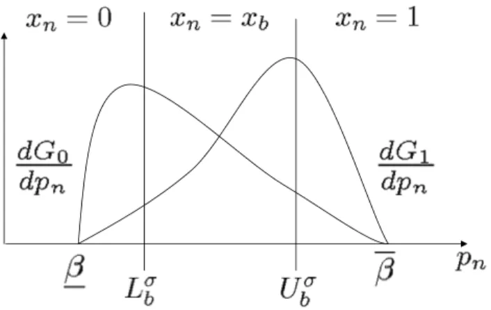
Proposition 3 Let B(n) = {b} for some agent n. Let σ ∈ Σ∗ _{be an equilibrium, and}

let Lσ

b andUbσ be given by Eq. (7). Then, agentn’s decision xn in equilibrium σ satisfies

xn=    0, if pn < Lσb xb, if pn ∈(Lσb, Ubσ) 1, if pn > Ubσ.

The proof is omitted since it is an immediate application of Lemma 1 [use Bayes’ Rule to determinePσ(θ= 1|xb =j) for each j ∈ {0,1}].

Note that the sequence{(Un, Ln)}only depends on{(Yn, Nn)}, and is thus

determin-istic. This reflects the fact that each individual recognizes the amount of information that will be contained in the action of the previous agent, which determines his own

Figure 3: The equilibrium decision rule when observing a single agent, illustrated on the private belief space.

decision thresholds. Individual actions are still stochastic since they are determined by whether the individual’s private belief is below Lb, above Ub, or in between (see Figure

3).

Using the structure of the equilibrium decision rule, the next lemma provides an expression for the probability of agent n making the correct decision conditional on his observing agentb < n, in terms of the private belief distributions and the thresholds Lσ b

and Uσ b.

Lemma 4 Let B(n) ={b} for some agent n. Let σ∈Σ∗ _{be an equilibrium, and let L}σ b and Uσ

b be given by Eq. (7). Then,

Pσ(xn=θ | B(n) ={b}) = 1 2 h G0(Lσb) + ¡ G0(Ubσ)−G0(Lσb) ¢ Nσ b + (1−G1(Ubσ)) + ¡ G1(Ubσ)−G1(Lσb) ¢ Yσ b i . Proof. By definition, agent n receives the same expected utility from all his possible equilibrium choices. We can thus compute the expected utility by supposing that the agent will choose xn = 0 when indifferent. Then, the expected utility of agent n (the

probability of the correct decision) can be written as Pσ(xn =θ | B(n) = {b})

=Pσ(pn≤Lσb |θ = 0)P(θ = 0) +Pσ(pn∈(Lσb, Ubσ], xb = 0 | θ = 0)P(θ = 0)

+Pσ(pn> Ubσ | θ= 1)P(θ = 1) +Pσ(pn∈(Lσb, Ubσ], xb = 1 |θ = 1)P(θ = 1).

The result then follows using the fact thatpnandxb are conditionally independent given

Using the previous lemma, we next strengthen Proposition 2 and provide a lower bound on the amount of improvement in the ex-ante probability of making the correct decision between an agent and his neighbor.

Lemma 5 Let B(n) ={b} for some agent n. Let σ∈Σ∗ _{be an equilibrium, and let L}σ b and Uσ

b be given by Eq. (7). Then,

Pσ(xn=θ | B(n) = {b}) ≥ Pσ(xb =θ) + (1−Nσ b )Lσb 8 G1 µ Lσ b 2 ¶ +(1−Y σ b )(1−Ubσ) 8 · 1−G0 µ 1 +Uσ b 2 ¶¸ .

Proof. In Lemma 3(b), let r=Lσ

b, z =Lσb/2, so that we obtain (1−Nσ b )G0(Lσb)≥YbσG1(Lσb) + (1−Nσ b)Lσb 4 G1 µ Lσ b 2 ¶ . Next, again using Lemma 3(b) and letting r=Uσ

b and w= (1 +Ubσ)/2, we have (1−Yσ b )[1−G1(Ubσ)]≥Nbσ[1−G0(σb)] + (1−Yσ b )(1−Ubσ) 4 · 1−G0 µ 1 +Uσ b 2 ¶¸ . Combining the preceding two relations with Lemma 4 and using the fact thatYσ

b +Nbσ =

2Pσ(xb =θ) [cf. Eq. (6)], the desired result follows.

The next lemma establishes that the lower bound on the amount of improvement in the ex-ante probability is uniformly bounded away from zero for unbounded private beliefs and when Pσ(xb =θ)<1, i.e., when asymptotic learning is not achieved.

Lemma 6 Let B(n) = {b} for some n. Let σ ∈ Σ∗ _{be an equilibrium, and denote}

α=Pσ(xb =θ). Then, Pσ(xn =θ | B(n) = {b})≥α+ (1−α)2 8 min ½ G1 µ 1−α 2 ¶ ,1−G0 µ 1 +α 2 ¶¾ . Proof. We consider two cases separately.

Case 1: Nσ

b ≤ α. From the definition of Lσb and the fact that Ybσ = 2α−Nbσ [cf. Eq.

(6)], we have Lσ_b = 1−N σ b 1−2Nσ b + 2α .

Sinceσis an equilibrium, we haveα≥1/2, and thus the right hand-side of the preceding inequality is a nonincreasing function of Nσ

b. Since Nbσ ≤ α, this relation therefore

implies that Lσ

b ≥ 1−α. Combining the relations 1−Nbσ ≥1−α and Lσb ≥1−α, we

obtain (1−Nσ b )Lσb 8 G1 µ Lσ b 2 ¶ ≥ (1−α) 2 8 G1 µ 1−α 2 ¶ . (8)