AIMS’ Journals
VolumeX, Number0X, XX200X pp.X–XX
A MAX-CUT APPROXIMATION USING A GRAPH BASED MBO SCHEME
Blaine Keetch and Yves van Gennip School of Mathematical Sciences
The University of Nottingham
University Park, Nottingham, United Kingdom, NG7 2RD.
(Communicated by the associate editor name)
Abstract. The Max-Cut problem is a well known combinatorial optimization problem. In this paper we describe a fast approximation method. Given a graphG, we want to find a cut whose size is maximal among all possible cuts. A cut is a partition of the vertex set ofGinto two disjoint subsets. For an unweighted graph, the size of the cut is the number of edges that have one vertex on either side of the partition; we also consider a weighted version of the problem where each edge contributes a nonnegative weight to the cut.
We introduce the signless Ginzburg–Landau functional and prove that this functional Γ-converges to a Max-Cut objective functional. We approximately minimize this functional using a graph based signless Merriman–Bence–Osher (MBO) scheme, which uses a signless Laplacian. We derive a Lyapunov func-tional for the iterations of our signless MBO scheme. We show experimentally that on some classes of graphs the resulting algorithm produces more accurate maximum cut approximations than the current state-of-the-art approximation algorithm. One of our methods of minimizing the functional results in an al-gorithm with a time complexity ofO(|E|), where |E|is the total number of edges onG.
1. Introduction.
1.1. Maximum cut. Given an undirected (edge-)weighted graphG= (V, E, ω), a cut V−1|V1 is a partition of the node set V into two disjoint subsets V−1 and V1.
The size of a cutC=V−1|V1, denoted bys(C), is the sum of all the weights corre-sponding to edges that have one end vertex inV−1 and one in V1. The maximum
cut (Max-Cut) problem is the problem of finding a cut C∗ such that for all cuts
C, s(C) ≤s(C∗). We call such a C∗ a maximum cut and say mc(G) :=s(C∗) is the maximum cut value of the graphG. The Max-Cut problem for an unweighted graph is a special case of the Max-Cut problem on a weighted graph which we ob-tain by assuming all edge weights are 1. Finding an unweighted graph’s Max-Cut is equivalent to finding a bipartite subgraph with the largest number of edges possible. In fact, for an unweighted bipartite graph mc(G) =|E|.
2010Mathematics Subject Classification. Primary: 05C85, 35R02, 35Q56; Secondary: 49K15, 68R10.
Key words and phrases. Graph algorithms, partial differential equations on graphs, Ginzburg-Landau functionals, NP Hard problems.
We would like to thank the EPSRC for supporting this work through the DTP grant EP/M50810X/1.
The Max-Cut problem is an NP-hard problem; assuming P 6= NP no solution can be acquired in polynomial time. There are a variety of polynomial time ap-proximation algorithms for this problem [25, 15, 53]. Some Max-Cut approxima-tion algorithms have a proven lower bound on their accuracy, which asserts the existence of a β ∈ [0,1] such that, for all output cuts C obtained by the algo-rithm, s(C) ≥ βmc(G). We call such a β a performance guarantee. For algo-rithms that incorporate stochastic steps, such a lower bound typically takes the form E[s(C)]≥βmc(G) instead, where E[s(C)] denotes the expected value of the size of the output cut.
In recent years a new type of approach to approximating such graph problems has gained traction. Models from the world of partial differential equations and variational methods that exhibit behaviour of the kind that could be helpful in solving the graph problem are transcribed from their usual continuum formulation to a graph based model. The resulting discrete model can then be solved using techniques from numerical analysis and scientific computing. Examples of problems that have successfully been tackled in this manner include data classification [11], image segmentation [16], and community detection [33]. In this paper we use a variation on the graph Ginzburg–Landau functional, which was introduced in [11], to construct an algorithm which approximately solves the Max-Cut problem on simple undirected weighted graphs.
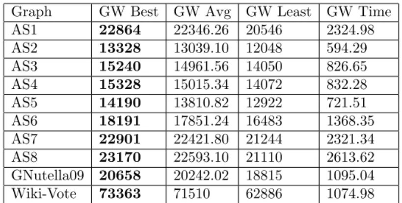
We compare our method with the Goemans–Williamson (GW) algorithm [25], which is the current state-of-the-art method for approximately solving the Max-Cut problem. In [25] the authors solve a relaxed Max-Cut objective function and inter-sect the solution with a random hyperplane in an-dimensional sphere. It is proven that if gw(C) is the size of the cut produced by the Goemans–Williamson algorithm, then its expected valueE[gw(C)] satisfies the inequalityE[gw(C)]≥βmc(G) where
β = 0.878 (rounded down). If the Unique Games Conjecture [36] is true, the GW algorithm has the best performance guarantee that is possible for a polynomial time approximation algorithm [37]. It has been proven that approximately solving the Max-Cut problem with a performance guarantee of 1617 ≈0.941 or better is NP-hard [52].
Finding mc(G) is equivalent to finding the ground state of the Ising Hamiltonian in Ising spin models [31], and 0/1 linear programming problems can be restated as Max-Cut problems [38].
1.2. Signless Ginzburg–Landau functional. Spectral graph theory [18] explores the relationships between the spectra of graph operators, such as graph Laplacians (see Section 2.1), and properties of graphs. For example, the multiplicity of the zero eigenvalue of the (unnormalised, random walk, or symmetrically normalised) graph Laplacian is equal to the number of connected components of the graph. Such properties lie at the basis of the successful usage of the graph Laplacian in graph clustering, such as in spectral clustering [58] and in clustering and classification methods that use the graph Ginzburg–Landau functional [11]
fε(u) := 1 2 X i,j∈V ωij(ui−uj)2+1 ε X i∈V W(ui). (1)
Here u:V →Ris a real-valued function defined on the node setV, with valueui
on node i, ωij is a positive weight associated with the edge between nodes i and
potential with minima atx=±1. In Section2.1we will introduce our setting and notation more precisely.
The method we use in this paper is based on a variation offε, we call thesignless Ginzburg–Landau functional: fε+(u) := 1 2 X i,j∈V ωij(ui+uj)2+1 ε X i∈V W(ui). (2) This nomenclature is suggested by the fact that the signless graph Laplacians are related tof+
ε in a similar way as the graph Laplacians are related tofε, as we will
see in Section2.1. Signless graph Laplacians have been studied because of the con-nections between their spectra and bipartite subgraphs [21]. In [32,55] the authors derive a graph difference operator and a graph divergence operator to form a graph Laplacian operator. In this paper we mimic this framework by deriving a signless difference operator and a signless divergence operator to form a signless Laplacian operator. Whereas the graph Laplacian operator is a discretization of the contin-uum Laplacian operator, the contincontin-uum analogue of the signless Laplacian is the subject of current and future research. Preliminary calculations for specific graph structures suggest that the continuum signless Laplacian is an integral operator [34].
The functional fε is useful in clustering and classification problems, because minimizers offε(in the presence of some constraint or additional term, to prevent trivial minimizers) will be approximately binary (with values close to±1), because of the double-well potential term, and will have similar values on nodes that are connected by highly weighted edges, because of the first term infε. This intuition
can be formalised using the language of Γ-convergence [20]. In analogy with the continuum case in [44, 45], it was proven in [55] that if ε↓0, then fε Γ-converges
to
f0(u) := (
2TV(u), ifuonly takes the values ±1,
∞, otherwise,
where TV(u) := 12P
i,j∈Vωij|ui−uj| is the graph total variation1. Together with
an equi-coercivity property, which we will return to in more detail in Section 4, this Γ-convergence result guarantees that minimizers offε converge to minimizers
of f0 as ε↓0. Ifuonly takes the values±1, we note that TV(u) = 2s(C), where
C = V−1|V1 is the cut given by V±1 := {i ∈ V : ui = ±1}. Hence minimizers uε of fε are expected to approximately solve the minimal cut problem, if we let V±1≈ {i∈V :uεi ≈ ±1}.
In Section4we prove thatf+
ε Γ-converges to a limit functional whose minimizers
solve the Max-Cut problem. Hence, we expect minimizersuεoffε+to approximately solve the Max-Cut problem, if we consider the cut C =V−1|V1, with V±1 ={i ∈ V :uεi ≈ ±1}.
1.3. Graph MBO scheme. There are various ways in which the minimization of
f+
ε can be attempted. One such way, which can be explored in a future publication,
is to use a gradient flow method. In the case offε the gradient flow is given by an
Allen–Cahn type equation on graphs [11,56],
dui dt =−(∆u)i− 1 εd −r i W 0(u i), (3)
1The multiplicative factor 2 inf
0above differs from that in [55] because in the current paper we choose different locations for the wells ofW.
where ∆uis a graph Laplacian ofu,di the degree of nodei, andr∈[0,1] a param-eter (see Section2.1for further details). This can be solved using a combination of convex splitting and spectral truncation. In the case offε+such an approach would
lead to a similar equation and scheme, with the main difference being the use of a signless graph Laplacian instead of a graph Laplacian.
In this paper, however, we have opted for an alternative approach, which is also inspired by similar approaches which have been developed for the fε case.
The continuum Merriman–Bence–Osher (MBO) scheme [41,42] involves iteratively solving the diffusion equation over a small time stepτ and thresholding the solution to an indicator function. For a short diffusion time τ this scheme approximates motion by mean curvature [10]. This scheme has been adapted to a graph setting [40,
56]. Heuristically it is expected that the outcome of the graph MBO scheme closely approximates minimizers offε, as the diffusion step involves solving dui
dt =−(∆u)i
and the thresholding step has a similar effect as the nonlinearity −1 εW
0(ui) in (3). Experimental results strengthen this expectation, however rigorous confirmation is still lacking.
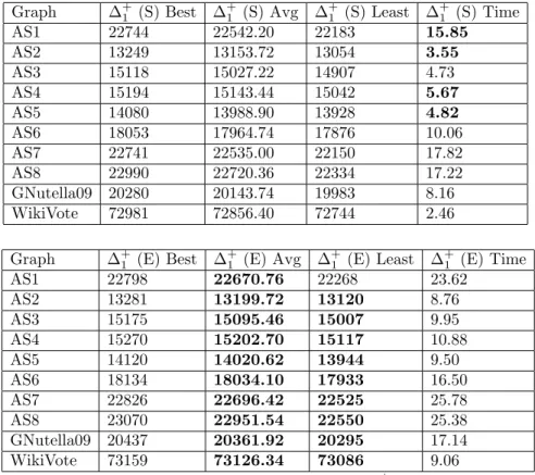
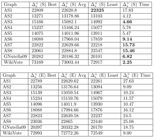
In order to approximately minimize fε+, and consequently approximately solve the Max-Cut problem, we use an MBO type scheme in which we replace the graph Laplacian in the diffusion step by a signless graph Laplacian. We use two methods to compute this step: (1) a spectral method, adapted from the one in [11], which allows us to use a small subset of the eigenfunctions, which correspond to the smallest eigenvalues of the graph Laplacian, and (2) an Euler method. Moreover, we show (Section 6) that this variant of the graph MBO scheme has a Lyapunov functional associated with it which Γ-converges to a Max-Cut objective functional (i.e. a functional whose minimizers solve the Max-Cut problem) as the signless ‘diffusion’ timeτ↓0.
The usefulness of (normalised) signless graph Laplacians when attempting to find maximum cuts can be intuitively understood from the fact that their spectra are in a sense (which is made precise in Proposition2) the reverse of the spectra of the corre-sponding (normalised) graph Laplacians. Hence, where a standard graph Laplacian driven diffusion leads to clustering patterns according to the eigenfunctions corre-sponding to its smallest eigenvalues, ‘diffusion’ driven by a signless graph Laplacian leads to patterns resembling the eigenfunctions corresponding to the smallest ei-genvalues of that signless graph Laplacian and thus the largest eiei-genvalues of the corresponding standard graph Laplacian.
1.4. Structure of the paper. In Section2we explain the notation we use in this paper and give some preliminary results. Section 3 gives a precise formulation of the Max-Cut problem and discusses the Goemans–Williamson algorithm in more detail. In Section 4 we introduce the signless graph Ginzburg–Landau functional
f+
ε and use Γ-convergence techniques to prove that minimizers of fε+ can be used
to find approximate maximum cuts. We describe the signless MBO algorithm we use to find approximate minimizers of fε+ in Section5 and discuss the results we get in Section 7. In Section 6 we derive a Lyapunov functional whose value is non-increasing along(MBO+)iterations, and show that subject to a re-scaling this functional Γ-converges to a total variation objective functional, which is shown to be related to maximum cuts. We analyse the influence of our parameter choices in Section8 and conclude the paper in Section9.
2.1. Graph based operators and functionals. In this paper we will consider non-empty finite, simple2, undirected graphsG= (V, E, ω) without isolated nodes, with vertex set (or node set)V, edge setE⊂V2and non-negative edge weightsω. We denote the set of all such graphs byG. By assumptionV has finite cardinality, which we denote by n := |V| ∈ N3. We assume a node labelling such that V =
{1, . . . , n}. Wheni, j∈V are nodes, the undirected edge betweeniandj, if present, is denoted by (i, j). The edge weight corresponding to this edge is ωij >0. Since Gis undirected, we identify (i, j) with (j, i) inE. Within this framework we can also consider unweighted graphs, which correspond to the cases in which, for all (i, j)∈E,ωij = 1.
We define V to be the set consisting of all node functions u : V → R and E
to be the set of edge functions ϕ : E → R. We will use the notation ui := u(i)
and ϕij := ϕ(i, j) for functions u ∈ V and ϕ ∈ E, respectively. For notational convenience, we will typically associateϕ∈ E with its extension toV2obtained by
settingϕij= 0 if (i, j)6∈E. We also extendωtoV2 in this way: if (i, j)6∈E, then ωij = 0. BecauseG∈ G is undirected, we have for all (i, j)∈E,ωij =ωji. Because
G∈ G is simple, for alli∈V, (i, i)∈/ E. The degree of a nodeiisdi:=P
j∈V ωij.
BecauseG∈ G does not contain isolated nodes, we have for alli∈V, di >0. As shown in [32], it is possible forV andE to be defined for directed graphs, but we will not pursue these ideas here.
To introduce the graph Laplacians and signless graph Laplacians we use and extend the structure that was used in [32,55,56]. We define the inner products on
V andE as hu, viV := X i∈V uividri, hϕ, φiE := 1 2 X i,j∈V ϕijφijω 2q−1 ij ,
wherer∈[0,1] andq∈[12,1]. Ifr= 0 anddi = 0, we interpretdri as 0. Similarly
forωij2q−1 and other such expressions below.
We define the graph gradient operator (∇:V → E) by, for all (i, j)∈E, (∇u)ij :=ω1ij−q(uj−ui).
We define the graph divergence operator (div :E → V) as the adjoint of the gradient, and a graph Laplacian operator (∆r:V → V) as the graph divergence of the graph
gradient: for alli∈V,
(divϕ)i:= 1 2d −r i X j∈V
ωijq(ϕji−ϕij), (∆ru)i:= (div(∇u))i=d−ir
X
j∈V
ωij(ui−uj).
(4) We note that the choicesr= 0 andr= 1 lead to ∆rbeing the unnormalised graph
Laplacian and random walk graph Laplacian, respectively [46,58]. Hence it is useful for us to explicitly incorporater in the notation ∆r for the graph Laplacian.
In analogy with the graph gradient, divergence, and Laplacian, we now define their ‘signless’ counterparts. We define the signless gradient operator (∇+:V → E)
by, for all (i, j)∈E,
(∇+u)ij :=ω 1−q
ij (uj+ui).
2By ‘simple’ we mean ’without self-loops and without multiple edges between the same pair of vertices’. Note that removing self-loops from a graph does not change its maximum cut.
3For definiteness we use the convention 06∈
Then we define the signless divergence operator (div+ : E → V) to be the adjoint of the signless gradient, and the signless Laplacian operator (∆+r :V → V) as the signless divergence of the signless gradient4: for alli∈V,
(div+ϕ)i:= 1 2d −r i X j∈V
ωijq(ϕji+ϕij), (∆+ru)i := (div+(∇+u))i=d−ir
X
j∈V
ωij(ui+uj).
By definition we have
h∇u, φiE =hu,divφiV, h∇+u, φiE =hu,div+φiV.
Proposition 1. The operators∆r :V → V and ∆+r :V → V are self-adjoint and positive-semidefinite.
Proof. Letu, v ∈ V. Since hu,∆rviV =h∇u,∇viE =h∆ru, viV and hu,∆+rviV =
h∇+u,∇+vi
E =h∆+ru, viV, the operators are self-adjoint. Positive-semidefiniteness follows fromhu,∆ruiV=h∇u,∇uiE ≥0 andhu,∆+ruiV =h∇+u,∇+uiE ≥0.
In the literature a third graph Laplacian is often used, besides the unnormalised and random walk graph Laplacians. This symmetrically normalised graph Laplacian [18] is defined by, for alli∈V,
(∆su)i:= 1 √ di X j∈V ωij √ui di −puj dj ! .
This Laplacian cannot be obtained by choosing a suitablerin the framework we introduced above, but will be useful to consider in practical applications. Analo-gously, we define the signless symmetrically normalised graph Laplacian by, for all
i∈V, (∆+su)i:= 1 √ di X j∈V ωij √ui di +puj dj ! .
There is a canonical way to represent a function u∈ V by a vector inRn with
components ui. The operators ∆r and ∆+r can then be represented by the n×n
matrices Lr := D1−r−D−rA and L+r := D1−r+D−rA, respectively. Here D is
the degree matrix, i.e. the diagonal matrix with diagonal entriesDii :=di, andA
is the weighted adjacency matrix with entriesAij:=ωij.
Similarly the operators ∆sand ∆+s are then represented byLs:=I−D−1/2AD−1/2
andL+s :=I+D−1/2AD−1/2, respectively, where Idenotes then×nidentity
ma-trix. Any eigenvalue-eigenvector pair (λ, v) ofLr,L+r, Ls, L+s corresponds via the
canonical representation to an eigenvalue-eigenfunction pair (λ, φ) of ∆r, ∆+r, ∆s,
∆+
s, respectively. We refer to the eigenvalue-eigenvector pair (λ, v) as an eigenpair.
For a vertex setS ⊂V, we define the indicator function (or characteristic func-tion)
χS := (
1, if i∈S,
0, if i /∈S.
4In some papers the spaceEis defined as the space of allskew-symmetricedge functions. We do not require the skew-symmetry condition here, hence∇+u ∈ E, having div+ act on∇+uis consistent with our definitions, and div+ϕis not identically equal to 0 for allϕ∈ E.
We define the inner product norms kukV := p
hu, uiV, kφkE := p
hφ, φiE which we use to define the Dirichlet energy and signless Dirichlet energy,
1 2k∇uk 2 E = 1 4 X i,j∈V ωij(ui−uj)2 and 1 2k∇ +uk2 E = 1 4 X i,j∈V ωij(ui+uj)2.
In particular we recognise that the graph Ginzburg–Landau functionalfε:V →R
from (1) and the signless graph Ginzburg–Landau functionalf+
ε :V →Rfrom (2) can be written as fε(u) =k∇uk2 E+ 1 ε X i∈V W(ui) and fε+(u) =k∇+uk2 E + 1 ε X i∈V W(ui).
It is interesting to note here an important difference between the functionalsfε
and f+
ε . Most of the results that are derived in the literature forfε (such as the
Γ-convergence results in [55]) do not crucially depend on the specific locations of the wells of W. For example, in fε the wells are often chosen to be at 0 and 1, instead of at−1 and 1. However, for fε+ we have less freedom to choose the wells without drastically altering the properties of the functional. The wells have to be placed symmetrically with respect to 0, because we want (ui+uj)2to be zero when
uiand uj are located in different wells. In particular, we see that placing a well at 0 would have the undesired consequence of introducing the trivial minimizeru= 0. This points to a second, related, difference. Whereas minimization of fε in the
absence of any further constraints or additional terms in the functional leads to trivial minimizers of the formu=cχV, wherec∈Ris one of the values of the wells
ofW (soc∈ {−1,1}for our choice ofW), minimizers off+
ε are not constant, if the
graph has more than one vertex. The following lemma gives the details.
Lemma 2.1. Let G ∈ G with n ≥ 2, let ε > 0, and let u be a minimizer of f+
ε :V →Ras in (2). Thenuis not a constant function.
Proof. Letc∈Randi∗∈V. Define the functions u,u¯∈ V byu:=cχV and
¯
ui:=
(
c, ifi6=i∗, −c, ifi=i∗. SinceW is an even function, we haveP
i∈V W(¯ui) =Pi∈V W(ui). Moreover, since
for allj∈V,ωi∗j= 0 oruj =−ui∗, we have
k∇+¯uk2 E = 1 2 X i∈V i6=i∗ X j∈V ωij(2c)2< 1 2 X i,j∈V ωij(2c)2=k∇+uk2 E.
The inequality is strict, because per assumption Ghas no isolated nodes and thus there is aj∈V such thatωi∗j>0. We conclude thatfε+(¯u)< fε+(u), which proves thatuis not a minimizer off+
ε .
We define the graph total variation TV :V →Ras TV(u) := max{hu,divϕiV:ϕ∈ E,∀i, j∈V |ϕij| ≤1}=
1 2
X
i,j∈V
ωijq|ui−uj|. (5)
The second expression follows since the maximum in the definition is achieved by
ϕ= sgn(∇u) [56]. We can define an analogous (signless total variation) functional TV+:V →R, using the signless divergence:
Lemma 2.2. Let u∈ V, thenTV+(u) =12P
i,j∈Vω q
ij|ui+uj|. Proof. Letϕ∈ E such that, for alli, j∈V,|ϕij| ≤1. We compute
hu,div+ ϕiV = 1 2 X i,j∈V ωqijui(ϕji+ϕij) = 1 2 X i,j∈V ωqijϕij(ui+uj) ≤1 2 X i,j∈V ωqij|ϕij||ui+uj| ≤1 2 X i,j∈V ωijq|ui+uj|.
Moreover, sinceϕ= sgn(∇+u) is an admissable choice forϕand hsgn ∇+u ,div+ ϕiV= 1 2 X i,j∈V ωijq|ui+uj|,
the result follows.
Note that the total variation functional that was mentioned in Section1.2 cor-responds to the choiceq= 1 in (5). This is the relevant choice for this paper and hence from now on we will assume thatq= 1. Note that the choice of qdoes not have any influence on the form of the graph (signless) Laplacians.
One consequence of the choice q = 1 is that TV and TV+ are now closely connected to cut sizes: IfS⊂V andC=S|Sc is the cut induced byS, then
TV (χS−χSc) = 2TV (χS) = 2s(C) and TV+(χS−χSc) =
X
i,j∈V
ωij−2s(C).
(6) We will give a precise definition ofs(C) in Definition3.1below.
Definition 2.3. LetG∈ G. ThenGis bipartite if and only if there exist A⊂V,
B⊂V, such that all the conditions below are satisfied:
• A∪B=V,
• A∩B=∅, and
• for all (i, j)∈E,i∈Aandj∈B, or i∈B andj ∈A. In that case we say thatGhas a bipartition (A, B).
Definition 2.4. An Erd¨os-R´enyi graphG(n, p) is a realization of a random graph generated by the Erd¨os-R´enyi model, i.e. it is an unweighted, undirected, simple graph withnnodes, in which, for all unordered pairs{i, j}of distinct i, j∈V, an edge (i, j)∈E has been generated with probabilityp∈[0,1].
2.2. Spectral properties of the (signless) graph Laplacians. We consider the Rayleigh quotients for ∆rand ∆+r defined, foru∈V, as
R(u) :=hu,∆ruiV kuk2V = k∇uk2 E kuk2V = 1 2 P i,j∈V ωij(ui−uj) 2 P i∈V d r iu2i , R+(u) :=hu,∆ + ruiV kuk2V = k∇+uk2 E kuk2V = 1 2 P i,j∈V ωij(ui+uj) 2 P i∈V d r iu 2 i ,
respectively. By Proposition1, ∆rand ∆+r are self-adjoint and positive-semidefinite
operators onV, so their eigenvalues will be real and non-negative. The eigenvalues of ∆rand ∆+r are linked to the extremal values of their Rayleigh quotients by the
min-max theorem [19,26]. In particular, if we denote by 0≤λ1≤. . .≤λnthe (possibly repeated) eigenvalues of ∆+, thenλ1= min
u1∈V\{0}
R+(u1) andλn= max un∈V\{0}
In the following proposition we extend a well-known result for the graph Lapla-cians [58] to include signless graph Laplacians.
Proposition 2. Let r∈[0,1]. The following statements are equivalent: 1. λis an eigenvalue ofL1 with corresponding eigenvector v;
2. λis an eigenvalue ofLs with corresponding eigenvector D1/2v; 3. 2−λis an eigenvalue ofL+1 with corresponding eigenvector v; 4. 2−λis an eigenvalue ofL+
s with corresponding eigenvector D1/2v; 5. λandv are solutions of the generalized eigenvalue problem Lrv=λD1−rv. Proof. For r = 1 the matrix representations of the graph Laplacian and signless graph Laplacian satisfy L+1 =I+D−1A= 2I−(I−D−1A) = 2I−L1. Henceλ
is an eigenvalue of L1 with corresponding eigenvector v if and only if 2−λis an eigenvalue ofL+1 with the same eigenvector.
Because Ls=D1/2L1D−1/2, λis an eigenvalue ofL1 with eigenvectorv if and
only if λ is an eigenvalue of Ls with eigenvector D1/2v. Moreover, since L+s =
2I−Ls, we have that 2−λis an eigenvalue ofL+
s with eigenvector D1/2v if and
only ifλis an eigenvalue ofLswith eigenvalueD1/2v.
Finally, forr∈[0,1], we haveLr=D1−rL1, henceλis an eigenvalue ofL1with
corresponding eigenvectorvif and only if Lrv=λD1−rv.
Inspired by Proposition 2, we define, for a given graph G∈ G and node subset
S⊂V, the rescaled indicator function ˜χS ∈ V, by, for allj∈V,
( ˜χS)j:=d 1 2
j (χS)j. (7)
Proposition 3. The graph G = (V, E, ω) ∈ G has k connected components if and only if∆∈ {∆r,∆s} (r∈[0,1]) has eigenvalue0 with algebraic and geometric multiplicity equal tok. In that case, the eigenspace corresponding to the0eigenvalue is spanned by
• the indicator functionsχSi, if ∆ = ∆r, or
• the rescaled indicator functionsχ˜Si (as in (7)), if ∆ = ∆s.
Here the node subsets Si ⊂V,i∈ {1, . . . , k}, are such that each connected compo-nent of Gis the subgraph induced by anSi.
Proof. We follow the proof in [58]. First we consider the case where ∆ = ∆r, r ∈ [0,1]. We note that ∆r is diagonizable in the V inner product and thus the
algebraic multiplicity of any of its eigenvalues is equal to its geometric multiplicity. In this proof we will thus refer to both simply as ‘multiplicity’.
For any functionu∈ V we have thathu,∆ruiV= 1 2
X
i,j∈V
ωij(ui−uj)2.We have that 0 is an eigenvalue if and only if there exists au∈ V \ {0} such that
hu,∆ruiV= 0. (8) This condition is satisfied if and only if, for alli, j∈V for whichωij >0,ui=uj. Now assume thatGis connected (henceGhask= 1 connected component), then (8) is satisfied if and only if, for alli, j ∈V, ui =uj. Therefore any eigenfunction corresponding to the eigenvalue λ1 = 0 has to be constant, e.g. u = χV. In particular, the multiplicity ofλ1is 1.
Now assume thatGhask≥2 connected components, letSi,i∈ {1, . . . , k}be the node sets corresponding to the connected components of the graph. Via a suitable
reordering of nodesGwill have a graph Laplacian matrix of the form Lr= L(1)r 0 · · · 0 0 L(2)r · · · 0 .. . ... . .. ... 0 0 · · · L(k)r ,
where each matrixL(i)r ,i∈ {1, . . . , k}corresponds to ∆rrestricted to the connected
component induced by Si. This restriction is itself a graph Laplacian for that component. Because eachL(i)r has eigenvalue zero with multiplicity 1,Lr(and thus
∆r) has eigenvalue 0 with multiplicityk. We can choose the eigenvectors equal to χSi fori∈ {1, . . . , k}by a similar argument as in thek= 1 case.
Conversely, if ∆r has eigenvalue 0 with multiplicity k, then Ghask connected
components, because ifGhasl6=kconnected components, then by the proof above the eigenvalue 0 has multiplicityl6=k.
For ∆swe use Proposition 2 to find that the eigenvalues are the same as those
of ∆r, with the corresponding eigenfunctions rescaled as stated in the result.
Proposition 4. Let G= (V, E, ω)∈ G have k connected components and let the node subsets Si ⊂ V, i ∈ {1, . . . , k} be such that each connected component is the subgraph induced by one of the Si. We denote these subgraphs by Gi. Let
∆+ ∈ {∆+r,∆+s} (r∈[0,1]) and let0≤k0 ≤k. Then ∆+ has an eigenvalue equal to 0 with algebraic and geometric multiplicity k0 if and only if k0 of the subgraphs Gi are bipartite. In that case, assume the labelling is such that Gi,i∈ {1, . . . , k0} are bipartite with bipartition (Ti, Si \Ti), where Ti ⊂ Si. Then the eigenspace corresponding to the 0 eigenvalue is spanned by
• the indicator functionsχTi−χSi\Ti, if ∆
+= ∆+ r, or
• the rescaled indicator functionsχT˜ i−χ˜Si\Ti (as in (7)), if∆
+= ∆+ s. Proof. First we consider the case where ∆+= ∆+
r, r∈[0,1]. For any vectoru∈ V
we have that hu,∆+ruiV = 1 2 X i,j∈V ωij(ui+uj)2.
Letk= 1, thenλ1= 0 is an eigenvalue if and only if there existsu∈ V \ {0}such that hu,∆+ruiV = 0. This condition is satisfied if and only if, for all i, j ∈ V for whichωij >0 we have
ui=−uj. (9)
We claim that this condition in turn is satisfied if and only if Gis bipartite. To prove the ‘if’ part of that claim, assumeGis bipartite with bipartition (A, Ac) for
some A ⊂ V, and define u∈ V such that u|A =−1 and u|Ac = 1. To prove the ‘only if’ statement, assume Gis not bipartite, then there exists an odd cycle inG
[12, Theorem 1.4]. Leti∈V be a vertex on this cycle, then by applying condition (9) to all the vertices of the cycle, we find ui =−ui = 0. SinceGis connected, it now follows, by applying condition (9) to all vertices in V, thatu= 0, which is a contradiction.
The argument above also shows that, if Gis bipartite with bipartition (A, Ac), then any eigenfunction corresponding toλ1 = 0 is proportional to u=χA−χAc. Therefore the eigenvalue 0 has geometric multiplicity 1. Since ∆+
in the V inner product the algebraic multiplicity of λ1 is equal to its geometric multiplicity.
Now let k≥2 and let Si, i ∈ {1, . . . , k} be the node sets corresponding to the connected components of the graph. Via a suitable reordering of nodes the graph
Gwill have a signless Laplacian matrix of the form
L+r = L(1)+ 0 · · · 0 0 L(2)+ · · · 0 .. . ... . .. ... 0 0 · · · L(k)+ ,
where each matrix L(i)+, i ∈ {1, . . . , k} corresponds to ∆+
r restricted to the
con-nected component induced by Si. This restriction is itself a signless Laplacian for that connected component. Hence, we can apply the casek= 1 to each component separately to find that the (algebraic and geometric) multiplicity of the eigenvalue 0 of ∆+r is equal to the number of connected components which are also bipartite.
If G hask0 ≤ k connected components which are also bipartite, then, without loss of generality, assume that these components correspond toSi,i∈ {1, . . . , k0}. Then the corresponding eigenspace is spanned by functionsu(i)=χ
Ti−χSi\Ti∈ V,
i ∈ {1, . . . , k0}, where Ti ⊂ Si and (Ti, Si\Ti) is the bipartition of the bipartite
component induced bySi. For ∆+
s we use Proposition2to find the appropriately rescaled eigenfunctions as
given in the result.
Corollary 1. The eigenvalues of∆1,∆+1 ,∆s, and∆+
s are in [0,2].
Proof. For ∆1 the proof can be found in [56, Lemma 2.5]. For completeness we
reproduce it here. By Proposition1we know that ∆1has non-negative eigenvalues.
The upper bound is obtained by maximizing the Rayleigh quotient R(u) over all nonzerou∈ V. Since (ui−uj)2≤2(u2i +u2j) we have that
max u∈V\{0} R(u) =u∈V\{max0} 1 2 P i,j∈V ωij(ui−uj) 2 P i∈V diu2i ≤ max u∈V\{0} 2P i∈V diu2i P i∈V diu2i = 2.
From Proposition 2 it then follows that the eigenvalues of the other operators are in [0,2] as well.
3. The Max-Cut problem and Goemans–Williamson algorithm.
3.1. Maximum cuts. In order to identify candidate solutions to the Max-Cut problem with node functions in V, we define the subset of binary {−1,1}-valued node functions,
Vb:={u∈ V :∀i∈V, ui∈ {−1,1}}.
For a given functionu∈ Vbwe define the setsVk :={i∈V, ui=k}fork∈ {−1,1}.
We say that the partitionC=V−1|V1is the cut induced byu. We define the set of all possible cuts,C:={C: there exists au∈ Vb such thatuinduces the cutC}.
Definition 3.1. LetG= (V, E, ω)∈ G and letV1 andV−1 be two disjoint subsets
ofV. The size of the cutC=V−1|V1is s(C) := X
i∈V−1 j∈V1
A maximum cut of Gis a cutC∗ ∈ C such that, for all cuts C∈ C, s(C)≤s(C∗). The size of the maximum cut is
mc(G) := max
C∈C s(C).
Note that if the cutCin Definition3.1is induced by u∈ Vb, then s(C) = 1
4hu,∆ruiV. (10)
Moreover, ifC=∅|V1or C=V−1|∅, thens(C) = 0.
Definition 3.2(Max-Cut problem). Given a simple, undirected graphG= (V, E, ω)∈ G, find a maximum cut forG.
For a given G ∈ G we have |E| <∞, hence a maximum cut for G exists, but note that this maximum cut need not be unique.
The cardinality of the set Vb is equal to the total number of ways a set of n
elements can be partitioned into two disjoint subsets, i.e. |Vb|= 2n. This highlights
the difficulty of finding mc(G) asnincreases. It has been proven that the Max-Cut problem is NP-hard [24]. Obtaining a performance guarantee of 1617 or better is also NP-hard [52]. The problem of determining if a cut of a given size exists on a graph is NP-complete [35].
3.2. The Goemans–Williamson algorithm. The leading algorithm for polyno-mial time Max-Cut approximation is the Goemans–Williamson (GW) algorithm [25], which we present in detail below in Algorithm(GW). A problem equivalent to the Max-Cut problem is to find a maximizer which achieves
max u 1 2 X i,j ωij(1−uiuj) subject to∀i∈V, ui∈ {−1,1}.
The GW algorithm solves a relaxed version of this integer quadratic program, by allowing uto be an n-dimensional vector with unit Euclidean norm. In [25] it is proved that the n-dimensional vector relaxation is an upper bound on the orig-inal integer quadratic program. This relaxed problem is equivalent to finding a maximizer which achieves
ZP∗ := max Y 1 2 X i,j∈V,i<j ωij(1−yij), (11)
where the maximization is over alln bynreal positive-semidefinite matricesY = (yij) with ones on the diagonal. This semidefinite program has an associated dual problem of finding a minimizer which achieves
ZD∗ :=1 2 X i,j∈V ωij+ 1 4γmin∈Rn X i∈V γi, (12)
subject toA+ diag(γ) being positive-semidefinite, whereAis the adjacency matrix ofGand diag(γ) is the diagonal matrix with diagonal entriesγi.
As mentioned in Section1.1, Algorithm (GW)is proven to have a performance guarantee of 0.878. In Algorithm(GW)below, we use the unit sphereSn :={x∈
Rn:kxk= 1}, wherek·kdenotes the Euclidean norm onRn. For vectorsw,w˜∈Rn,
w·w˜ denotes the Euclidean inner product.
Other polynomial time Max-Cut approximation algorithms can be found in [15, 53]. Because of the high proven performance guarantee of (GW), we focus
Algorithm (GW): The Goemans–Williamson algorithm
Data: The weighted adjacency matrixA of a graphG∈ G, and a tolerance
ν.
Relaxation step: Use semidefinite programming to find approximate solutions ˜ZP∗ and ˜ZD∗ to (11) and (12), respectively, which satisfy
|Z˜P∗ −Z˜D∗|< ν. Use an incomplete Cholesky decomposition on the matrix
Y that achieves ˜Z∗
P in (11) to find an approximate solution to w∗∈argmax w∈(Sn)n 1 2 X 1≤i,j,≤n i<j ωij(1−wi·wj).
Hyperplane step: Letr∈Sn be a random vector drawn from the
uniform distribution on Sn. Define the cutC:=V−1|V1, where V1:={i∈V|wi·r≥0} and V−1:=V \V1.
on comparing our algorithm against it. In [53] the authors use the eigenvector cor-responding to the smallest eigenvalue of ∆+0, showing that thresholding this eigen-vector in a particular way achieves a Max-Cut performance guarantee ofβ= 0.531, which with further analysis was improved to β = 0.614 [51]. Algorithms which provide a solution in polynomial time exist if the graph is planar [30], if the graph is a line graph [29], or if the graph is weakly bipartite [27]. Comparing against [53,30,29,27] is a topic of future research.
4. Γ-convergence of f+
ε . In (2) we introduced the signless Ginzburg–Landau
functional f+
ε : V → R. In this section we prove minimizers of fε+ converge to
solutions of the Max-Cut problem, using the tools of Γ-convergence [13].
We need a concept of convergence inV. Since we can identify V with Rn and
all norms onRn are topologically equivalent, the choice of a particular norm is not
of great importance. For definiteness, however, we say that sequence{uk}k∈N⊂ V converges to a u∞ ∈ V in V if and only if kukˆ −uˆ∞kV → 0 as k → ∞, where ˆ
uk,uˆ∞∈Rn are the canonical vector representations ofuk,u∞, respectively. We will prove thatfε+ Γ-converges to the functionalf
+
0 :V →R∪ {+∞}, which
is defined as
f0+(u) := (P
i,j∈V ωij|ui+uj|, ifu∈ V b,
+∞, ifu∈ V \ Vb. (13)
Lemma 4.1. Let G∈ G. For everyu∈ Vb, let Cu ∈ C be the cut induced by u, then for allu∈ V,
f0+(u) = ( 2P i,j∈V ωij−4s(Cu), if u∈ V b, +∞, if u∈ V \ Vb. In particular, ifu∗∈argmin u∈V
fε+(u), thenu∗∈ Vb andCu∗ is a maximum cut ofG.
Proof. Because, foru∈ Vb, f+
0(u) = 2TV +
(u) (with q= 1), the result follows by (6).
Lemma 4.2. Let G ∈ G and ε > 0. There exist minimizers for the functionals fε+:V →Randf0+:V →R∪ {+∞} from (2)and (13), respectively. Moreover, if u∈ V is a minimizer off0+, thenu∈ Vb.
Proof. The potentialW satisfies a coercivity condition in the following sense. There exist aC1>0 and aC2such that, for allx∈R,
|x| ≥C1⇒C2(x2−1)≤W(x). (14)
Combined with the fact thatk∇+uk
E ≥0, this shows thatfε+ is coercive. Sincefε+
is a (multivariate) polynomial, it is continuous. Thus, by the direct method in the calculus of variations [20, Theorem 1.15]f+
ε has a minimizer inV.
Sincen≥1,Vb6=∅and thus inf u∈Vf
+
0(u)<+∞. In particular, any minimizer of f0+ has to be inVb. Since|Vb|<∞the minimum is achieved.
Lemma 4.3. Let G ∈ G and let f+ ε and f + 0 be as in (2) and (13), respectively. Thenf+ ε Γ-converges tof +
0 asε↓0in the following sense: If{εk}k∈Nis a sequence
of positive real numbers such that εk↓0 ask→ ∞ andu0∈ V, then the following lower bound and upper bound conditions are satisfied:
(LB) for every sequence {uk}∞k=1 ⊂ V such thatuk →u0 ask → ∞, it holds that f0+(u0)≤lim inf
k→∞ f
+ εk(uk);
(UB) there exists a sequence {uk}∞
k=1 ⊂ V such that uk → u0 as k → ∞ and f0+(u0)≥lim sup
k→∞
f+ εk(uk).
Proof. This proof is an adaptation of the proofs in [55, Section 3.1]. Note that fε+(u) = 1 2 X i,j∈V ωij(ui+uj)2+wε(u), where we definewε:V →Rby wε(u) := 1 ε X i∈V W(ui).
First we prove thatwεΓ-converges tow0 asε↓0, where
w0(u) :=
(
0, ifu∈ Vb,
+∞, ifu∈ V \ Vb.
Let{εk}k∈N be a sequence of positive real numbers such thatεk ↓0 ask→ ∞and
u0∈ V.
(LB) Note that, for all u∈ V we have wε(u)≥0. Let {uk}∞
k=1 be a sequence
such thatuk→u0as k→ ∞. First we assume that u0∈ Vb, then w0(u0) = 0≤lim inf
k→∞ wεk(uk).
Next suppose that u0∈ V \ Vb, then there is an i∈V such that (u0)i 6∈ {−1,1}.
Since uk →u0 as k → ∞, for every η >0 there is anN(η)∈ Nsuch that for all
k≥N(η) we have thatdr i|(u0)i−(uk)i|< η. Define ¯ η:= 1 2d r
imin{|1−(u0)i|,| −1−(u0)i|}>0,
then, for allk≥N(¯η),
|1−(uk)i| ≥ |1−(u0)i| − |(u0)i−(uk)i| ≥ 1 2|1−(u0)i|>0.
Similarly, for all n≥N(¯η),| −1−(uk)i| ≥ 1
2| −1−(u0)i|>0. Hence, there is a c >0 such that, for all k≥N(¯η),|(uk)i| ≤1−c. Thus there is a C >0 such that, for allk≥N(¯η),W((uk)i)≥C. It follows that
lim inf
k→∞ wεk(uk)≥lim infk→∞ 1
εkW((uk)i) =∞=w0(u0).
(UB) Ifu0∈ V \Vb, thenw0(u0) and the upper bound condition is trivially satisfied.
Now assumeu0∈ Vb. Define the sequence{uk}∞
k=1 by, that for allk∈N,uk =u0.
Then, for all k ∈ N, wεk(uk) = 0 and thus lim sup
k→∞
wεk(uk) = 0 = w0(u0). This concludes the proof thatwε Γ-converges tow0 asε↓0.
It is known that Γ-convergence is stable under continuous perturbations [20, Proposition 6.21], [13, Remark 1.7]; thus wε+p Γ-converges to w0+p for any continuousp:V →R. Sinceu7→ 12
P
i,j∈V ωij(ui+uj)
2 is a polynomial and hence
a continuous function on V, we find that, as ε ↓ 0, f+
ε Γ-converges to g : V → R∪ {+∞}, where g(u) := 1 2 X i,j∈V ωij(ui+uj)2+w0(u).
Ifu∈ V \Vb, theng(u) = +∞. Ifu∈ Vb, then, for alli, j∈V, (ui+uj)2= 2|ui+uj|,
hence 1 2 X i,j∈V ωij(ui+uj)2= X i,j∈V
ωij|ui+uj|.
Thusg=f0+ and the theorem is proven. Lemma 4.4. Let G ∈ G and let f+
ε be as in (2). Let {εk}k∈N ⊂ (0,∞) be a
sequence such that εk ↓ 0 as k → ∞, then the sequence {f+
εk}k∈N satisfies the
following equi-coerciveness property: If {uk}k∈N⊂ V is a sequence such that there
existsC >0 such that, for all k∈N,fε+k(uk)< C, then there exists a subsequence
{uk0}k0∈
N⊂ {uk}k∈N and au0∈ Vb such that uk0 →u0 ask→ ∞.
Proof. This proof closely follows [55, Section 3.1]. From the uniform bound f+
εk(uk) < C, we have that, for all k ∈ N and all
i ∈ V, 0 ≤ W((uk)i) ≤ C. Because of the coercivity property (14) of W, the
uniform bound onW((uk)i) gives, for alli∈V, boundedness of{dri(uk)2i}k∈N and thus {uk}k∈N is bounded in the V-norm. The result now follows by the Bolzano-Weierstrass theorem.
With the Γ-convergence and equi-coercivity results from Lemmas 4.3 and 4.4, respectively, in place, we now prove that minimizers offε+ converge to solutions of the Max-Cut problem.
Theorem 4.5. Let G∈ G. Let {εk}k∈N ⊂(0,∞)be a sequence such that εk ↓ 0 as k→ ∞and, for each k∈N, let fε+k be as in (2) and let uεk be a minimizer of
f+
εk. Then minu∈Vf
+
εk(u)→minu∈Vf
+
0(u)as k→ ∞. Furthermore, there existsu0 ∈ Vb and a subsequence{uεk0}k0∈N⊂ {uεk}k∈N, such that kuεk0 −u0kV→0 as k
0→ ∞.
Moreover,u0∈argmin
u∈V
f0+(u), wheref0+ is as in (13). In particular, ifCu0 ∈ C is the cut induced byu0, thenCu0 is a maximum cut ofG.
Proof. It is a well-known result from Γ-convergence theory [20, Corollary 7.20], [13, Theorem 1.21] that the equi-coercivity property of {fεk}k∈N from Lemma 4.4
combined with the Γ-convergence property of Lemma 4.3 implies that min u∈Vf + εk(u) converge to min u∈Vf +
0 (u) ask→ ∞, and, up to taking a subsequence, minimizers of f+ εk converge to a minimizer off + 0 ask→ ∞. By Lemma4.2, ifu0∈argmin u∈V f0+(u), then u0 ∈ Vb. By Lemma 4.1, the cut Cu0 induced by u0 is a maximum cut of G.
5. The signless MBO algorithm.
5.1. Algorithm. One way of attempting to find minimizers offε+is via its gradient flow [6]. This is, for example, the method employed in [11] to find approximate minimizers offε. In that case the gradient flow is given by a graph-based analogue of the Allen–Cahn equation [5]. To find theV-gradient flow offε+ we compute the
first variation of the functionalf+
ε: fort∈R, u, v∈ V, we have d dtf + ε(u+tv)|t=0=h∆+ru, viV+ 1 εhD −rW0◦u, vi V,
where we used the notation (D−rW0◦u)i=d−i rW0(ui). This leads to the following V-gradient flow: for all i∈V,
(du i dt =−(∆ + ru)i−1εdi−rW0(ui), fort >0, ui= (u0)i, fort= 0. (15) Sincef+
ε is not convex, ast→ ∞the solution of theV-gradient flow is not
guaran-teed to converge to a global minimum, and can get stuck in local minimizers. In this paper we will not attempt to directly solve the gradient flow equation. That could be the topic of future research. Instead we will use a graph MBO type scheme, which we call the signless MBO algorithm. It is given in(MBO+). Despite there currently not being any rigorous results on the matter, the outcome of this scheme is believed to approximate minimizers of f+
ε. The original MBO scheme
(or threshold dynamics scheme) in the continuum was introduced to approximate motion by mean curvature flow [41,42]. It consists of iteratively applying (Ntimes) two steps: diffusing a binary initial condition for a time τ and then thresholding the result back to a binary function. In the (suitably scaled) limitτ ↓0,N → ∞, solutions of this process converge to solutions of motion by mean curvature [10]. It is also known that solutions the continuum Allen–Cahn equation (in the limitε↓0) converge to solutions of motion by mean curvature [14]. Whether something similar is true for the graph MBO scheme or graph Allen–Cahn equation [56] or something analogous is true for the signless graph MBO scheme are as of yet open questions, but it does suggest that solutions of the MBO scheme (signless MBO scheme) could be closely connected to minimizers offε(f+
ε). In practice, the graph MBO scheme
has proven to be a fast and accurate method for tackling approximate minimization problems of this kind [40,11].
We see in(MBO+)that in the signless diffusion step the equation that is solved is the gradient flow equation from (15) without the double well potential term. Since we expect the double well potential term in (15) to force the solution to take values close to ±1, the signless diffusion step in (MBO+) is followed by a thresholding step. Note that, despite our choice of nomenclature, the signless graph ‘diffusion’ dynamics is expected to be significantly different from standard graph diffusion.
In Figures 1 and 2 we show the minimization of fε+ using (MBO+) with the
Algorithm (MBO+):The signless graph MBO algorithm Data: A signless graph Laplacian ∆+∈ {∆+
0,∆ +
1,∆+s}corresponding to a
graphG∈ G, a signless diffusion timeτ >0, an initial condition
µ0:=χS
0−χS0c corresponding to a node subsetS0⊂V, a time step dt, and a stopping criterion toleranceη.
Output: A sequence of functions{µj}N
j=0⊂ Vb giving the signless MBO
evolution ofµ0, a sequence of corresponding cuts{Cj}N j=0⊂ C
and their sizes{s(Cj)}N
j=0⊂[0,∞), with largest values∗.
forj= 1 to stopping criterion is satisfied,do
Signless diffusion step: Computeu∗(τ), whereu∗∈ V is the solution of the initial value problem
(du(t)
dt =−∆
+u(t), fort >0,
u(0) =µj. (16)
Threshold step: Define µj∈ Vb by, fori∈V,
µji :=T(u∗i(τ)) := (
1, ifu∗i(τ)>0,
−1, ifu∗i(τ)≤0. (17)
Define the cutCj :=Vj
−1|V j 1, whereV j ±1:={i∈V :µ j i =±1}and computes(Cj). SetN=j. if kµj−µj −1k2 2 kµjk2 2 < η then Stop
Find the largest cut size: Sets∗:= max1≤j≤Ns(Cj).
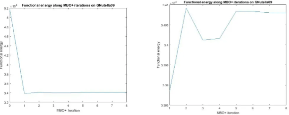
GNutella09 graph (see Section7.3). The(MBO+)iteration numbersjare indicated along thex-axis. They-axis shows the value off+
ε(µj). What we see in both figures
is that the overall tendency is for the(MBO+) algorithm to decrease the value of
fε+(µj), however, in some iterations the value increases. This is why in(MBO+)we output the cut size which is largest among all iterations computed and use that as the final output, if it outperforms the cutCwhich(MBO+)returns. Alternatively, in order to save on computing memory, one could also keep track of the largest cut size found so far in each iteration and discard the other cut sizes, or accept the final cut size s(CN) as approximation tos∗ . The result we report in this paper are all based on the outputs∗.
In our experiments we choose the stopping criterion toleranceη = 10−8.
5.2. Spectral decomposition method. In this paper we will compare two im-plementations of the (MBO+) algorithm, which differ in the way they solve (16) for t ∈ [0, τ]. In the next section we consider an explicit Euler method, but first we discuss a spectral decomposition method. In order to solve (16) we use spectral decomposition of the signless graph Laplacian ∆+ ∈ {∆+0,∆1+,∆+s}. Let λk ≥0, k ∈ {1, . . . , n} be the eigenvalues of ∆+. We assume λ1 ≤ λ2 ≤ . . . λn and list eigenvalues multiple times according to their multiplicity. Letφk ∈ Vbe an eigen-function corresponding to λk, chosen such that {φk}nk=1 is a set of orthonormal
Figure 1. The valuefε+(µj) as a function of the iteration number jin the(MBO+)scheme on AS8Graph, using the spectral method and ∆+1, with K = 100, and τ = 20. The left hand plot shows the initial condition and all iterations of the (MBO+) scheme on AS8Graph, where as the right hand plot displays the 3rd to the final iterations of the(MBO+)scheme on AS8Graph.
Figure 2. The valuefε+(µj) as a function of the iteration number jin the(MBO+)scheme on the GNutella09 graph, using the spec-tral method and ∆+1, with K = 100, and τ = 20. The left hand plot shows the initial condition and all iterations of the(MBO+)
scheme on GNutella09, where as the right hand plot displays all it-erations of the(MBO+)scheme on GNutella09, without the initial condition.
functions inV. We then use the decomposition
u∗(τ) = n X k=1 e−λkτhφk, u(0)i Vφk (18) to solve (16).
For ∆+s we use the Euclidean inner product instead of the V inner product in
(18), because the Laplacian ∆+s is not of the form as given in (4). The optimal
choice for τ with respect to the cut size obtained by(MBO+)is a topic for future research. Based on trial and error, we decided to use τ = 20 in the results we
present in Section7, when using ∆+1 or ∆+s as our operator. We useτ = λ40 n when using ∆+0 as our operator, where λn is the largest eigenvalue of ∆+0. The division ofτ by half of the largest eigenvalue of ∆+0 is justified in Section5.4. In Section 8
we investigate how cut sizes change with varyingτ.
A computational advantage of the spectral decomposition method is that we do not necessarily need to use all of the eigenvalues and eigenfunctions of the signless Laplacian. We can use only the K eigenfunctions corresponding to the smallest eigenvalues in our decomposition (18). To be explicit, doing this replacesnin (18) byK. In Section8we show how increasingKbeyond a certain point has little effect on the size of the cut obtained by(MBO+)for three examples. We refer to using the
Keigenfunctions corresponding to the smallest eigenvalues in the decomposition as spectral truncation.
By Proposition2, we can compute theKsmallest eigenvaluesλk(k∈ {1, . . . , K})
of ∆+1 and ∆+
s by first computing theKlargest eigenvalues ˆλl(l∈ {n−K+1, . . . , n})
of ∆1and ∆srespectively instead and then settingλk = 2−λnˆ −k+1. There is not a
similar property for ∆+0 however. Proving upper bounds on the largest eigenvalues of ∆0 and ∆+0 is an active area of research. [28,49,59].
We use the MATLAB eigs function to calculate the K eigenpairs of the sign-less Laplacian. This function [39] uses the Implicitly Restarted Arnoldi Method (IRAM) [50], which can efficiently compute the largest eigenvalues and correspond-ing eigenvectors of sparse matrices. The function eigs firstly computes the or-thogonal projection of the matrix you want eigenpairs from, and a random vector, onto the matrix’sK-dimensional Krylov subspace. This projection is represented by a smaller K×K matrix. Theneigs calculates the eigenvalues of thisK×K
matrix, whose eigenvalues are called Ritz eigenvalues. The Ritz eigenvalues are computed efficiently using a QR method [23]. Computationally these Ritz eigenva-lues typically approximate the largest eigenvaeigenva-lues of the original matrix. The time complexity of IRAM is currently unknown, but in practice it produces approximate eigenpairs efficiently.
If the matrix of which the eigenvalues are to be computed is symmetric, the MAT-LABeigs function simplifies to the Implicitly Restarted Lanczos Method (IRLM) [17], therefore typically in practice eigs will usually compute the eigenvalues and eigenfunctions of ∆+
s faster than those of ∆ + 1.
Using the IRLM for computing the eigenpairs of ∆+0 corresponding to its smallest eigenvalues is inefficient. In our experiments using the MATLAB eigfunction to calculate all eigenpairs of ∆+0 and choosing theK eigenpairs corresponding to the smallest eigenvalues for the decomposition (18) was faster than using the IRLM to calculate the K eigenpairs of ∆+0. Hence, the results discussed in this paper are obtained witheigwhen using ∆+0 and eigswhen using ∆+1 or ∆+s.
If we use the MATLAB eigs function when using our spectral decomposition method we cannot a priori determine the time complexity for (MBO+), because practical experiments have shown the complexity of the IRAM and IRLM methods is heavily dependent on the matrix to which they are applied [47]. If we choose to use the MATLABeigfunction then the time complexity of (MBO+)isO(n3),
which is the time complexity of computing all eigenpairs of an n×n matrix. All other remaining steps of(MBO+) require fewer operations to compute.
5.3. Explicit Euler method. We also compute the solution of (16) fort∈[0, τ] using an explicit finite difference scheme,
(
um+1=um−∆+umdt, form∈ {0,1, . . . , M},
u0=u(0) (19)
for the same choice ofτ as in (18). For M ∈N,dt= Mτ, and we setu
∗(τ) =uM.
IfG∈ G then (MBO+)using the Euler method will have a time complexity of
O(|E|), because of the sparsity of the signless Laplacian matrix. When zero entries are ignored, the multiplication of the vector um by ∆+ takes 4|E|+ 2noperations
to compute. Since G ∈ G has no isolated nodes, |E| ≥ n−1, therefore, when n
is large enough, 4|E|>2n and hence the time complexity of the multiplication is
O(|E|). All other remaining steps in(MBO+)using the Euler method require fewer operations to compute.
In Section 8.3 we show some results for (MBO+) when solving (16) using an implicit finite difference scheme, comparing against the results of(MBO+)obtained using (19) to solve (16).
5.4. (MBO+) pinning condition. For (MBO+) we have that choosing τ too small causes trivial dynamics in the sense that, for anyj,µj =µ0in (MBO+). In this section we prove a result which shows that such a τ is inversely proportional to the largest eigenvalue of the signless Laplacian chosen for(MBO+).
We define d− := min
i∈V di, andd+ := maxi∈V di. Let ∆
+ ∈ {∆+ 0,∆ + 1,∆ + s}, then the operator normk∆+k V is defined by k∆+kV:= sup u∈V\{0} k∆+ukV kukV
We define the maximum norm ofV bykukV,∞:= max{|ui|:i∈V}. Lemma 5.1. Let∆+∈ {∆+
0,∆ +
1,∆+s}. The operator normk∆+kV and the largest
eigenvalueλn of ∆+ are equal. This implies that, for allu∈ V, k∆+ukV≤λnkukV.
Proof. See [56, Lemma 2.5].
Lemma 5.2. The normsk · kV andk · kV,∞are equivalent, with optimal constants
given by
d
r
2
−kukV,∞≤ kukV≤ kχVkVkukV,∞.
Proof. See [56, Lemma 2.2].
Theorem 5.3. Let G ∈ G, and let λn be the largest eigenvalue of the signless Laplacian∆+∈ {∆+0,∆+1,∆+s}. Let S0⊂V,µ0:=χS0−χS0c, and let µ
1∈ Vb be the result of applying one (MBO+)iteration toµ0. If
τ < λ−n1log(1 +d r 2 −kχVk− 1 V ), thenµ1=µ0.
Proof. This proof closely follows the proof of a similar result in [56, Section 4.2]. Ifke−τ∆+µ0−µ0k
V,∞<1, thenµ1=µ0. Using Lemma5.2, we compute
ke−τ∆+µ0−µ0kV,∞≤d −r 2 − ke− τ∆+ µ0−µ0kV≤d −r 2 − ke− τ∆+ −IdkVkµ0kV.
Moreover, since hχS0, χSc 0iV = 0, we have kµ 0k2 V = kχS0k 2 V+kχSc 0k 2 V = kχS0 + χSc 0k 2 V=kχVk2V.
Using the triangle inequality and the submultiplicative property (see [48] for example) ofk · kV, we computeke−τ∆ + −IdkV ≤P∞k=1 1 k!(τk∆ +k V)k =eλnτ−1. Therefore, ifτ < λ−1 n log(1 +d r 2 −kχVk−1), thenµ1=µ0.
As stated in Section5.2, we choose τ = 20 as diffusion time for(MBO+) using ∆+1 or ∆+
s, and τ = 40
λn when using (MBO+) with ∆
+
0 as the choice of operator.
This is due toτ = 20 often being too large when using(MBO+)with ∆+0. Choosing
τ= 20 for(MBO+)using ∆+0 causes the solution to converge tou(τ) = 0 to machine precision. We therefore chooseτ = λ40
n for ∆
+
0 since5.3 implies a suitable choice
of τ for (MBO+) with respect to obtaining non-trivial output cuts is inversely proportional to the largest eigenvalue of the chosen operator ∆+. Sinceλn= 2 for
∆+1 and ∆+ s we choose to divideτ by λn 2 for ∆ + 0.
6. Γ-convergence of the Lyapunov functional for (MBO+) evolutions. 6.1. Lyapunov functional. In this section, in (20), we introduce a Lyapunov functional for (MBO+). We prove that, when properly rescaled, this functional Γ-converges to the signless total variation. In our setup and proofs we follow earlier similar work in [56, 57] which in turn was inspired by results in the continuum setting obtained in [22]. We first introduce some needed notation.
Define the space of functionsK:={u∈ V:∀i∈V, ui∈[−1,1]}. In analogy with [56] we use our operators to define a graph curvature using our signless definitions. IfC=S|Sc we define the signless normal of a set by
νSij:= sgn((∇+(χS−χS c)ij) = 1, ifi, j∈S, −1, ifi, j∈Sc, 0, otherwise,
and our curvature as
(κq,r,+S )i := (div+νS)i =d−ir (P j∈Sω q ij, ifi∈S, −P j∈Scω q ij, ifi∈S c.
By direct computation we note that ∆+(χ
S−χSc)i= 2κ 1,r,+
S . We define the volume
of a node setS⊆V by VolS:=kχSk2 V= X i∈S dri.
Proposition 5. LetG∈ Gand forr∈[0,1], let∆+= ∆+
r. Then, for allu∈ V\{0} we have that hu, e−τ∆+ui V = X i∈V e−τ λihu, φii2 V >0.
Proof. This has been proved in [57] using the operator ∆ instead of ∆+. Our proof here, which we include for completeness, is similar. We expand u on the
V-orthonormal basis formed by the eigenfunctions{φi}n i=1: hu, e−τ∆+ uiV= * X i∈V hu, φii V φi, X j∈V e−τ λjhu, φji V φj + V = X i,j∈V e−τ λjhu, φii V hu, φjiV δij= X i∈V e−τ λihu, φii2 V,
whereδij is the Kronecker delta function. This expression is strictly positive since
uis not the zero function.
Proposition 6. Let G∈ G and letC∈ C. Then for S⊆V we have that
TV+(χS−χSc) =hκ1,r,+S , χS−χSciV.
Proof. By direct computation we show that
hκq,r,+S , χS−χSciV =dri X i∈S (X j∈S d−i rωqij)−dr i X i∈Sc (−X j∈Sc d−irωqij) = X i,j∈S ωijq+ X i,j∈Sc ωijq.
By settingq= 1 we see that ifC=S|Sc, then
X i,j∈S ωijq+ X i,j∈Sc ωqij = X i,j∈V ωij−2( X i∈S,j∈Sc ωij) = X i,j∈V ωij−2s(C) = TV+(χS−χSc).
Proposition 7. Let G ∈ G and, for r ∈ [0,1], let ∆+ = ∆+r. Let (λi, φi)
(i ∈ {1, . . . , n}) denote the eigenpairs of ∆+, where the eigenfunctions are V -orthonormal. Then forS ⊆V we have that
TV+(χS−χSc) = 1 2 X i∈V λihχS−χSc, φii2V.
Proof. By Proposition6we have
TV+(χS−χSc) =hκ1,r,+S , χS−χSciV, which can be expressed as
* κ1,r,+S ,X i∈V hχS−χSc, φiiVφi + V =X i∈V hκ1,r,+S , φiiVhχS−χSc, φiiV. We have that ∆+(χS−χS c) = 2κ1,r,+S , therefore TV+(χS−χSc) = 1 2 X i∈V h∆+(χS−χSc), φiiVhχS−χSc, φiiV. Since ∆+ is self-adjoint in theV inner product by Proposition1, we have that
1 2 X i∈V h∆+(χS−χSc), φiiVhχS−χSc, φiiV = 1 2 X i∈V hχS−χSc,∆+φiiVhχS−χSc, φiiV = 1 2 X i∈V hχS−χSc, λiφiiVhχS−χSc, φiiV= 1 2 X i∈V λihχS−χSc, φii2V.
Lemma 6.1. LetG∈ G,τ >0, and forr∈[0,1], let∆+= ∆+r. DefineJτ:V →R
by
Jτ(u) :=−hu, e−τ∆+ui
V+ VolV. (20)
Then the following hold.
1. The functional Jτ(u)is strictly concave and Fr´echet differentiable. 2. Its derivative at u∈ V in the direction of v∈ V is given by
dJτu(v) =−2he−τ∆+ u, viV.
3. Letµ0:=χ
S0−χSc
0 for someS0⊂V and let{µ j}N
j=1 be a sequence generated by (MBO+). For allj∈ {1, . . . , N},µj minimizesdJτµj−1(·)overK:
µj∈argmin
v∈K
dJτµj−1(v). (21)
4. For all j∈ {1, . . . , N},Jτ(µj)≤Jτ(µj−1), with equality attained if and only if µj=µj−1.
Remark 1. The final property in the lemma above shows that Jτ is a Lyapunov functional for(MBO+). All the results in Lemma6.1remain true if a constant term is added to Jτ. In particular, they remain true if the term VolV is removed from (20). We included this term in the definition ofJτ, however, because it is needed in Section6.2for our Γ-convergence results.
Proof of Lemma 6.1. In [56, Lemma 4.5, Proposition 4.6] and [57, Lemma 5.5] the authors derive similar Lyapunov functionals for two graph based MBO schemes similar to(MBO+). This proof is similar to those proofs.
We first compute the Gateaux derivative atu∈ V in the direction ofv∈ V. Let
ε∈R, then
dJτu(v) := dJτ(u+εv)
dε |ε=0=−2he
−τ∆+ u, viV,
where we have applied the fact that ∆+, and thus alsoe−τ∆+ are self-adjoint. Since u7→dJu
τ(v) is continuous,Jτ is also Fr´echet differentiable. Moreover, ifv∈ V\{0}
the second directional derivative is given by
d2Jτ(u+εv)
dε2 |ε=0 =−2hv, e
−τ∆+vi
V
which, by Proposition5, is strictly negative. ThereforeJτ is strictly concave. To prove the third property, letj∈ {1, . . . , N}. Thenµjis generated by(MBO+)
and thus it takes values in{−1,1}. Letµ∗∈ K\{µj}and leti∈V be such thatµ∗
i 6= µji. Assume first thatµji = 1 and henceµ∗
i ∈[−1,1). Then, by (16), (17), we have e−τ∆+ µj−1 i >0 and thus −2e−τ∆+µj−1 i driµji <−2e−τ∆+µj−1 i driµ∗i. If, on the other hand i ∈ V is such that µji = −1 and hence µ∗i ∈ (−1,1], then e−τ∆+µj−1 i ≤ 0 and thus −2e−τ∆+µij−1driµj i ≤ −2e−τ∆+µj−1 i driµ∗i. Hence, for all µ∗ ∈ K \ {µj}, we have dJµj−1
τ (µj) ≤ dJµ
j−1
τ (µ∗) and therefore µj is a minimizer.
SinceJτ is strictly concave anddJµ
j−1
τ is linear we conclude that if µj 6=µj+1,
then Jτ(µj+1)−Jτ(µj)< dJµ j τ (µ j+1 −µj) =dJτµj(µj+1)−dJτµj(µj)≤0.
The inequality follows from (21). Ifµj+1=µj thenJ
Remark 2. Our proof of (21) above also shows that minimizers in (21) need not be unique: at verticesi∈V wheree−τ∆+µj−1
i6= 0 any minimizer has to agree with µjobtained by(MBO+), but at verticesiwheree−τ∆+µj−1
i= 0 minimizers can
take any value in [−1,1].
6.2. Γ-convergence proof. Letr∈ [0,1] and ∆+ = ∆+r. Forτ >0 we define a
rescaled version ofJτ, restricted toK: define ˆJτ :K →R∪ {∞} by ˆJτ := τ1 Jτ|K, i.e. ˆ Jτ(u) :=−1 τhu, e −τ∆+ui V+ 1 τVolV. (22)
We prove that forτ↓0 this functional Γ-converges to ˆJ0:K →R∪ {∞}defined by
ˆ
J0(u) := (
2TV+(u), ifu∈ Vb,
+∞, ifu∈ K\Vb, (23)
whereq= 1. Note that ˆJ0= f0+
K, wheref
+
0 is as in Lemma4.1. We use the same
notion of convergence inV is the same as in Section4.
Lemma 6.2. Let G ∈ G and let Jˆτ and Jˆ0 be as in (22) and (23), respectively. ThenJτˆ Γ-converges toJ0ˆ asτ↓0in the following sense: If {τk}k∈Nis a sequence
of positive real numbers such thatτk ↓0as k→ ∞ andu0∈ K, then the following lower bound and upper bound conditions are satisfied:
(LB) for every sequence {uk}∞
k=1 ⊂ K such thatuk →u0 as k→ ∞, it holds that
ˆ
J0(u0)≤lim inf
k→∞ ˆ
Jτk(uk); (UB) there exists a sequence {uk}∞
k=1 ⊂ K such that uk → u0 as k → ∞ and
ˆ
J0(u0)≥lim sup
k→∞ ˆ
Jτk(uk).
Proof. (LB) By Proposition5 we can express (22) as ˆ Jτ(u) =− 1 τ X i∈V e−τ λihu, φii2 V+ 1 τVolV =− X i∈V e−τ λi−1 τ hu, φ i i2V−1 τ X i∈V hu, φii2V+1 τVolV. Since τk ↓ 0 as k→ ∞, we have e −τkλi−1 τk → d dte −tλi t=0 as k→ ∞. Moreover,
sinceuk→u0ask→ ∞, we deduce that, for alli∈V,−lim
k→∞ e−τkλi−1 τk huk, φii2 V= λihu0, φii2V.It follows that lim inf k→∞ ˆ Jτ(uk) =X i∈V
λihu0, φii2V+ lim inf
k→∞ 1 τk volV − X i∈V huk, φii2V ! . (24)
Sinceuk∈ K, we have, for alli∈V, (uk)2i ≤1 and thus
X
i∈V
huk, φii2V=hu
2

![1 (Prop 2 en 1 yl) 3 {[3 (pyridin 4 yl) 4,5 dihydroisoxazol 5 yl]methyl} 1H anthra[1,2 d]imidazole 2,6,11(3H) trione](data:image/gif;base64,R0lGODlhAQABAIAAAP///wAAACH5BAEAAAAALAAAAAABAAEAAAICRAEAOw==)