MULTISCALE FORECASTING
MODELS BASED ON SINGULAR
VALUES FOR NONSTATIONARY TIME
SERIES
Lida Barba Maggi, Doctorado en Ingeniería Informática. Pontificia Universidad Católica
de Valparaíso.
Resumen—Time series are valuable sources of information for supporting planning activities. Transport, fishery, economy and finances are predominant sectors concerned into obtaining information in advance to improve their productivity and efficiency. During the last decades diverse linear and nonlinear forecasting models have been developed for attending this demand. However the achievement of accuracy follows being a challenge due to the high variability of the most observed phenomena. In this research are proposed two decomposition methods based on Singular Value Decomposition of a Hankel matrix (HSVD) in order to extract components of low and high frequency from a nonstationary time series. The proposed decomposition is used to improve the accuracy of linear and nonlinear autoregressive models. The evaluation of the proposed forecasters is performed through data coming from transport sector and fishery sector. Series of injured persons in traffic accidents of Santiago and Valparaíso and stock of sardine and anchovy of central-south Chilean coast are used. Further, for comparison purposes, it is evaluated the forecast accuracy reached by two decomposition techniques conventionally used, Singular Spectrum Analysis (SSA) and decomposition based on Stationary Wavelet Transform (SWT), both joint with linear and nonlinear autoregressive models. The experiments shown that the proposed methods based on Singular Value Decomposition of a Hankel matrix in conjunction with linear or nonlinear models reach the best accuracy for one-step and multi-step ahead forecasting of the studied time series.
Index Terms—Singular Value Decomposition, Forecasting, Linear models, Nonlinear Models, Wavelet Decomposition, Singular Spectrum Analysis.
F
1.
I
NTRODUCTIONA
time series is a collection of observations measured sequentially through the time. A time series is continue when it is collected continuously over some time interval, whereas it is discrete when the collection interval is constant. In this work only discrete time series will be used in order to approach the vast majority of time series applications. Examples of discrete time series are (i) the inflation rates during successive months or years, (ii) the electricity consum-ption for successive one-hour periods, (iii) the number of injured people in traffic accidents during successivedays, weeks, months, etc.
It has been demonstrated that time series are valuable sources of information for supporting planning acti-vities and designing strategies for decision-making. Multiple demand coming from diverse sectors such as, transport, fishery, economy, and finances are concerned into obtaining information in advance to improve their productivity and efficiency. Unfortunately often is ob-served the presence of high variability in a time series, this situation obey to the presence oftrend,seasonal variation,cyclic fluctuation, orirregular fluctuation.
During the last decades have been developed nume-rous forecasting models to explain the behavior of an observed phenomena. It is well known that an analysis method works quite well when the variation is domina-ted by a regular linear trend and/or regular seasonality [1], complementary a process is called second-order stationaryif its first and second moments (mean and covariance) are finite and do not change through time, and when these conditions are not fulfilled the process is callednonstationary.
Analysis in the frequency domain is usually based on the examination of cyclical or periodical content. The methods of the frequency domain are based on Fourier transform that allow us to identify the number of frequency components and detect the dominant cyclic observations. However Fourier transform-based methods have limitations in that they require an as-sumption of stationarity and produce no information associated with time [2]. Whereas the time domain techniques include the analysis of the correlation struc-ture, development of models that describe the manner in which such data evolve in time, and forecasting future behavior [3].
ARIMA (Autoregressive Integrated Moving Average) was introduced by Box et al. [4] for forecasting of nonstationary time series. ARIMA implementations are observed electricity [6], environment [8], [9], and tourism [10]. ARIMA implements D processes of differentiation for transforming a nonstationary time series in stationary, most time series are stationarized taking the first difference (D=1). An ARMA(P,Q) model is the generalization of an ARIMA(P,D,Q) model, wherePis the order of the autoregressive part (number of autoregressive terms) andQ is the order of the moving average part (number of lagged forecast errors).
On the other hand nonlinear relationships are often modelled by nonlinear models. The Artificial Neural Network (ANN) and the Support Vector Machine (SVM) are popular methods of artificial intelligen-ce that are implemented in regression problems. For instance, three typical ANN techniques were probed by Li and Shi (2010) for one-step ahead wind speed forecasting [11], after testing, the Back Propagation-based model was considered the best model for one site, while the Radial Basis Function was the best option for other site; the research concludes that it is not recommended to employ only one type of
ANN model in wind speed forecasting. Another re-presentative example is the prices variation range, Laboissiere et al. [12] modeled stock prices of power distribution companies through an ANN based on Levenberg-Marquardt (LM), different Multilayer Per-ceptron (MLP) topologies were evaluated iteratively with opening and closing prices and other correlated variables for finding of best configuration for short-term horizon. An ANN implementation implies to take some decisions, after several tests, about some para-meters such as network topology, signal propagation method, activation function, weights updating, hidden levels, and numbers of nodes; besides, a specific confi-guration cannot be generalized, even in similar studies. Support Vector Regression (SVR) is another type of nonlinear model, SVR is a parsimonious alternative for forecasting which uses the same principles as the SVM introduced by Vapnik [13], and its basic idea is to use the linear model to implement nonlinear class boundaries through some nonlinear mapping of the in-put vector into the high-dimensional feature space; the unique mathematical formulation of SVR guarantees a computationally tractable global optimal solution [14]. Hybrid models are a recent solution to deal with nonstationary processes. Hybrid models combine pre-processing techniques with conventional linear and nonlinear models, two of them, widely implemented, are Singular Spectrum Analysis (SSA) and Discrete Wavelet Transform (DWT). These techniques extract components from observed signals, the components are smoother than the original signal which improve forecast models.
SSA is a nonparametric spectral estimation method used to decompose a time series into a sum of trend, cyclical component, seasonal component, and an irre-gular component. SSA is defined in four steps, embed-ding, Singular Value Decomposition (SVD), grouping, and diagonal averaging [27]. The beginning of the SSA method is attributable to some authors [28], [29], [30], the SSA flexibility is favorable to apply it in diverse areas, such as climatic, meteorological, or geophysics [31], [32], energy [33], industrial production [34], tourist arrivals [35], trade [36], and some well-known time series with different structures and characteristics, nonstationary, nonlinear and chaotic [15].
The Wavelet theory was originated in 1984 with the discovery of Grossman and Morlet in the quantum physics context [16], later Stephane Mallat presented
Multiresolution Analysis (MRA) to digital signal pro-cessing [17]. For discrete wavelet analysis, orthogonal wavelets and biorthogonal wavelets have been com-monly used, being Daubechies [18] the most popular wavelet family. In the wavelet domain, the effective decomposition level must be selected in advance to im-prove the performance of linear or nonlinear models; a common practice is to use three decomposition levels. Wavelet decomposition in conjunction with artificial intelligence can further improve the efficiency of auto-regressive models in many areas, such as, hydrology [19], transportation systems [20], and public health [21].
In this research are proposed two decomposition met-hods based on Singular Value Decomposition of a Hankel matrix (HSVD) in order to extract components of low and high frequency from a nonstationary time series. The proposed decomposition is used to improve the accuracy of linear and nonlinear autoregressive models. More precisely, the contributions of this work are the following:
One-step ahead forecastingbased on Singular Value Decomposition of a Hankel matrix for
linearforecasting models.
Multi-step ahead forecastingbased on Singu-lar Value Decomposition of a Hankel matrix forlinearforecasting models.
One-step ahead forecastingbased on Singular Value Decomposition of a Hankel matrix for
nonlinearforecasting models.
Multi-step ahead forecastingbased on Singu-lar Value Decomposition of a Hankel matrix fornonlinearforecasting models.
This contribution was validated with time series coming from traffic accidents and fishery stock. Six time series obtained from CONASET [37] and SER-NAPESCA were used, they are the following:
1. Weekly sampling from 2003:1 to 2012:12 of
injuredpersons in traffic accidents in Valpa-raíso.
2. Weekly sampling from 2000:1 to 2014:12 of
injuredpersons in traffic accidents inSantiago
due to 10 principal causes related to inap-propriate behaviorof drivers, passengers and pedestrians.
3. Weekly sampling from 2000:1 to 2014:12 of
injuredpersons in traffic accidents inSantiago
due to 10 secondary causes related to inap-propriate behaviorof drivers, passengers and pedestrians.
4. Weekly sampling from 2000:1 to 2014:12 of
injuredpersons in traffic accidents inSantiago
due to causes related to road deficiencies, mechanical failures and undetermined causes. 5. Monthly sampling from 1958:1 to 2011:12 of anchovy catches at center-south coast of Chile.
6. Monthly sampling from 1949:1 to 2011:12 of
sardine catchesat center-south coast of Chile. Systematic comparisons are performed between the proposed methods with respect to decomposition tech-niques widely used, Singular Spectrum Analysis and Stationary Wavelet Transform. More precisely the ele-ments of comparisons are the following:
Forecasting based onSSAin conjunction with theARmodel.
Forecasting based onSSAin conjunction with a feedforward ANN based on Levenberg-Marquardt.
Forecasting based onSWTin conjunction with theARmodel.
Forecasting based on SWT in conjunction with a feedforwardANNbased on Levenberg-Marquardt.
This work is structured as follows. In section 2 is Time Series Analysis via Linear and Nonlinear models. In section 3 is presented Preprocessing Time Series based on Singular Value Decomposition of a Hankel matrix (HSVD), Multilevel SVD (MSVD) and Wavelet Decomposition (SWT). In section 4 are presented a Case Study for forecasting of traffic accidents, models AR and ANN based on HSVD, MSVD and SWT are provided. Finally, from section 6 the works is conclu-ded and highlighted future directions of the research.
1.1. Objectives
1.1.1. General Objective
Develop two extraction methods of low and high frequency components from nonstationary time series for improving the accuracy of linear and nonlinear forecasting models.
1.1.2. Specific Objectives
Design a method to extract components of low and high frequency from time series based on Singular Value Decomposition of a Hankel matrix.
Design a method to extract components of low and high frequency from time series based on Multilevel Singular Value Decomposition of a Hankel matrix.
Evaluate the performance of the proposed met-hods of components extraction in forecasting of nonstationary time series.
Compare the performance of the proposed methods of components extraction with res-pect to Singular Sres-pectrum Analysis and Sta-tionary Wavelet Transform for forecasting of nonstationary time series.
1.2. Justification
Strongly nonlinear and nonstationary process pre-sent high variability that can not be modelled by clas-sic estimation methods. Conventional models based on ARIMA and ANNs have been found insufficient because of the highly complicated nature of a some time series [22].
The ANNs application has spread to several areas of knowledge and thus various strategies have been im-plemented in order to improve their performance. The ANN performance depends of more than one decisions such as, the appropriate selection of transfer functions and activation, the variation in the input dimension, the number of hidden nodes, and the learning algo-rithm. There are diverse neural networks architectures such as feed-forward, recurrent, radial basis, among others. Unluckily, there is no general methodology or guideline to determine which neural network is the best fit for modeling a specific structural analysis problem. Consequently, the best network is attained through trial and error [23].
Hybrid models are a recent solution to deal with nonstationary processes. Hybrid models combine pre-processing techniques with conventional linear and nonlinear models, some of them widely implemented are Singular Spectrum Analysis (SSA), Discrete Wa-velet Transform (DWT), and Empirical Mode Decom-position (EMD). These techniques extract components from observed signals, the components are smoother
than the original signal which improve the forecast accuracy. Although the flexibility of SSA and DWT allows their usage in a wide range of forecast pro-blems, there is a lack of standard methods to select their parameters. SSA requires an effective window length for extracting intrinsic components, and DWT requires to select the wavelet function, which in prin-ciple is unknown. EMD frequently has the appearance of mode mixing, which is defined as a single IMF either consisting of signals of widely disparate scales, or a signal of a similar scale residing in different IMF components [24].
This study is justified by the need of decomposition models that guarantees flexibility for its application on nonstationary time series and forecasting accuracy via conventional models.
Furthermore there are time series coming from relevant sectors as transport and fishery that have been sparsely researched. More precisely police and government institutions make monitoring and promote prevention activities to encourage responsible attitude of drivers, passengers, and pedestrians for avoid the occurrence of traffic accidents. Whereas fishery industry makes monitoring of marine species for controlled fishing.
1.3. Research Question
Is it possible to improve the accuracy of conventionally accepted linear and nonlinear forecasting methods?
Can the Singular Value Decomposition techni-que to enhance the performance of conventio-nally accepted decomposition techniques?
1.4. Hypothesis
The extraction methods of low and high fre-quency components based on Singular Value Decomposition of a Hankel matrix achieve more accuracy in multi-step ahead forecasting than methods based on Singular Spectrum Analysis and Stationary Wavelet Transform. The hypothesis will be validated by means of compu-tational simulation based on nonstationary time series coming from traffic accidents and fisheries stock.
2.
T
IMES
ERIESA
NALYSISThe idea of deterministic time series was a contri-bution of Yule in 1927, which launched the notion that
every time series can be regarded as the realization of a stochastic process. The concepts of Autoregressive (AR) and Moving Average (MA) models were also formulated by Yule.
Linear autoregressive models are not able to deal with two features in several series, nonlinearly and nonstationarity. ARIMA model proposed by George P. Box and Gwilym M. Jenkins in their book published in 1970 presented an alternative to overcomes a part of the problem. ARIMA transforms a nonstationary time series in stationary through differentiation processes, however the nonlinearly follows present.
Artificial Neural Networks (ANNs) were originated in 1943 by McCulloch and Pitts. The first ANN, known as Perceptron, which was a linear model with connec-tions of fix weight. As the Perceptron was not able to generalize the learning with nonlinear functions, Rumelhart and McCelland presented Backpropagation (BP) algorithm for a Multilayer Perceptron (MLP). Backpropagation have been extensively applied since its creation. From BP new algorithms based on the descent method have been discovered to accelerate the convergence.
On the other hand, time series preprocessing has gai-ned popularity in the last decade. Data preprocessing contributes highly in the performance of forecasting models. Preprocessing prepares the data for forecas-ting.
Singular Value Decomposition is a data preprocessing technique with almost one century of history [39]. However, actually SVD follows being used for diverse purposes. Popular application of SVD are denoising, features reduction, and image compression. Important advances have been also observed for signal-noise separation.
Singular Spectrum Analysis and Wavelet Decomposi-tion in this research are techniques used to validate our proposal.
In certain situations, it may be difficult to ascertain whether or not a given series is nonstationary. This is because there is often no sharp distinction between stationarity and nonstationarity when the nonstationary boundary is nearby. In the Box-Jenkins methodology, the Autocorrelation Function (ACF) is often used for identifying, selecting, and assessing conditional mean models (for discrete, univariate time series data).
2.1. Linear Autoregressive Models
Linear time series modelling are commonly asso-ciated with a family of linear stochastic models which are referred as ARIMA (Autoregressive Integrated Moving Average) models. ARIMA is also known as Box-Jenkins methods due to the work of George P. Box and Gwilym M. Jenkins. ARIMA is in fact a culmi-nation of the research of many prominent statisticians, starting with the pioneering work of Yule in 1927, who employed an Autoregressive (AR) model of order 2 to model yearly sunspot numbers.
Time series analysis by means of linear models are conditioned to deal with stationary data or at least weakly stationary. Stationary models assume that the process remains in statistical equilibrium with pro-babilistic properties that do not change over time, in particular varying about a fixed constant mean level and with constant variance.
Mostnaturally generatedsignals are nonstationary, in that the parameters of the system that generate the signals, and the environments in which the signals propagate, change with time and/or space [7]. Some researches consider that natural processes are inhe-rently nonstationary, although apparent nonstationarity in a given time series may constitute only a local fluctuation of a process that is in fact stationary on a longer time scale or viceversa.
There are some methods to convert a nonstationary ti-me series in stationary. ARIMA impleti-mentsD proces-ses of differentiation, most time series are stationarized taking the first difference (D=1). An ARMA(P,Q) model is the generalization of an ARIMA(P,D,Q) model, wherePis the order of the autoregressive part (number of autoregressive terms) and Q is the order of the moving average part (number of lagged forecast errors).
The simplest analysis is performed through an autore-gressive model of orderPand with i.i.d. innovations
ε (having zero mean and at least finite second-order moments) for the data-generating process,
b X(n+1) = P
∑
i=1 αiZi+ε(n+1), (1)wherePis the model order,αiisith coefficient andZi
An ARMA (P,Q) model is defined with b X(n+1) = P
∑
i=1 αiZi+ Q∑
i=1 βiεi+ε(n+1), (2)where Xb(n+1) is the future value of the observed
time series,αi is thei-th coefficient of the AR term
Zi. βi denotes the ith coefficient of the MA term εi
andε(n+1)is a source of randomness which is called white noise. The AR termsZi are the columns of the
regressor matrix Z= (Z1, . . . ,ZP).
The coefficients of AR and ARMA models have been commonly estimated by Least Squares (LS) method and by Maximum Likelihood Estimation (MLE). On the one hand LS computes the parameters that provide the most accurate description of the data, the sum of square errors computed between observed values and estimated values must be minimized. On the other hand MLE is a method to seek the probability distribution that makes the observed data most likely.
Least Squares method is one of the oldest technique of modern statistics which origin is related with the work of Legendre and Gauss. In a standard formulation, a set of pairs of observations x,y, is used to find a function that relates the observations. A linear function is defined to estimate the values of a set of dependent variablesY from the values of independent variables
X, as follows:
b
Y=a+bX, (3) where a is the intercept and b is the slope of the regression line. If the intercept is zero, the equation is reduced to
b
Y=bX. (4)
The LS method estimates thebparameters according to the rule that those values must minimize the sum of residual squares computed between the observed values and the predicted values,
ε= N
∑
i=1 (yi−ybi) 2, (5a) = N∑
i=1 (yi−bxi)2, (5b)where ε is the value to be minimized. Taking the
derivative ofε with respect tob, and setting them to zero gives the following equation:
∂ ε ∂b= ∂(∑i(y2i−2bxiyi+b2x2i)) ∂b , (6a) b=∑ixiyi ∑ix2i . (6b)
Extending the solution to a higher degree polynomial is straightforward. In matrix form, linear models are given by the formula
b
X=αZ, (7)
whereXis aN×1 vector of results (for univariate time series),α is aP×1 vector of coefficients (with P<
N), and Z is the regressor matrix ofN×Pdimension, which is named design matrix for the model.
The Moore-Penrose pseudoinverse matrix [40] X† is
computed to obtain the coefficients matrixα, it is
α=Z†X. (8) In general, LS estimates tend to differ from MLE estimates, especially for data that are not normally distributed such as proportion correct and response time.
Maximum Likelihood Estimation (MLE) was first in-troduced by Fisher in 1922, although he first presen-ted the numerical procedure in 1912. MLE consists of choosing from among the possible values for the parameter, the value which maximizes the probability of obtaining the sample which was obtained [41]. In the practice, from original observations (yi for
i = 1, . . . ,N) through an ARIMA(P,D,Q) model is generated a new differentiated series X(n) =
x1, . . . ,xN. The parameters set is defined with θ =
(α1, . . . ,αP,β1, . . . ,βQ,σ2). The joint probability den-sity function (PDF) is denoted with
f(xN,xN−1, . . . ,x1;θ). (9)
Thelikelihood functionis this joint PDF treated as a function of the parametersθ given the dataX(n):
L(θ|X) =f(xN,xN−1, . . . ,x1;θ). (10)
The maximum likelihood estimator is
b
θ =arg max L(θ|X(n)), θ∈Θ, (11) where Θis the parameters space. The term arg max refers to the arguments at which the function output is
as large as possible.
For simplifying calculations, it is customary to work with the natural logarithm ofL, which is commonly referred to as the log-likelihood function. Because the logarithm is a monotonically increasing function, the logarithm of a function achieves its maximum value at the same points as the function itself, and hence the log-likelihood can be used in place of the likelihood in maximum likelihood estimation and related techniques. Finding the maximum of a function often involves taking the derivative of a function and solving for the parameter being maximized, and this is often easier when the function being maximized is a log-likelihood rather than the original likelihood function.
MLE is preferred to LS when the probability density function is known (generally normal) or easy to obtain through computable form. There is a situation in which LS and MLE intersect. This is when observations are independent of one another and are normally distributed with a constant variance. In this case, maximization of the log-likelihood is equivalent to minimization of SSE, and therefore, the same parameter values are obtained under either LS or MLE [25].
2.2. Artificial Neural Networks
The first Artificial Neural Network was proposed by McCulloch and Pitts in 1943, it was designed to use connections with a fixed set of weights. In the early 1960s, some researchers among them Rosenblatt, Block, Minsky and Paper developed a learning algo-rithm for a device known as Perceptron which conver-gence was warranted if the connections weights could be adjusted. In 1969 Minsky and Papert, determined that the Perceptron was not able to generalize the learning with nonlinear functions. The limitation of the Perceptron, paralyzed for a long time the researching in the field of ANNs.
Between 1980 and 1986, the PDD group consisting of Rumelhart and McCelland, publish the book Parallel Distributed Processing: Explorations in the Micros-tructure of Cognition. Backpropagation (BP) algorithm was shown in the publication as an algorithm for multilayer and nonlinear neural network known as Multilayer Perceptron (MLP).
Artificial Neural Network (ANN) is commonly used for referencing a MLP. ANN is in general an infor-mation processing system that has certain performance characteristics in common with biological neural net-works.
The performance of an ANN depends of different elements, such as, structure, activation function and learning algorithm. Classification, prediction, and ima-ges recognition are common tasks of an ANN. The power of an ANN approach lies not necessarily in the elegance of the particular solution, but rather in the generality of the network to find its own solution to particular problems, given only examples of the desired behavior [26].
The common structure of an ANN has three layers, input, hidden, and output [26]. The presence of a hid-den layer together with a nonlinear activation function, gives it the ability to solve many more problems than can be solved by a net with only input and output layers.
An autoregressive ANN of three layers uses the lagged terms zi at the input layer, they are weighted with
respect to the hidden layer, at the output of the hidden layer is applied the activation function. At the output layer is obtained the estimated valueXb(n+1),
b X(n+1) = Q
∑
j=1 bjYH j, (12a) YH j= f P∑
i=1 wjizi ! , (12b)where Z1, . . . ,ZP are the input neurons, and
w11, . . . ,wP1, . . . ,wPQ are the nonlinear weights of
the connections between the inputs and the hidden neurons. Whereas b1, . . . ,bQ are the weights of the
connections between the hidden neurons and the output (under the assumption that there is an unique output). The common activation function is sigmoid, which is expressed with
f(x) = 1
1+e−x (13)
The ANN for an univariate process is denoted with
ANN(P,Q,1), withP inputs, Q hidden nodes, and 1 output. The parameterswi j andbjare updated during
the training via learning algorithm. At each iteration the weights are adapted to reach the minimization of the errors.
The learning algorithms are gradient-based and gradient-free (or derivative-free). Algorithms of first order are those where the first derivative of the objec-tive function is computed to adapt the neural network weights, whereas algorithms of second order are those that compute the second derivative.
Backpropagation is a gradient-based also known as steepest-descent algorithm which repeatedly adjusts the weights of the connections in the network so as to minimize a measure of the difference between the actual output vector. Standard steepest descent is given below,
∆ωt=lr
∂Et
∂ ωt, (14a)
ωt+1=ωt−∆ωt, (14b)
where ∆ωt is called delta rule, and determines the
amount of weight update based on the gradient di-rection along with a step size. ω is the matrix of weights and bias,tis the number of epoch (repetition),
lr is the learning rate (in standard steepest descent
BP, lr is constant). E is the Performance Function
which is arbitrary (Egenerally has a quadratic form, by example Mean Square Error MSE). The neural network is trained until the stopping criteria is reached; stop criteria might be the number of epochs, the maximum iteration time, the minimum level of error performance, or the performance gradient falls below the minimum gradient predefined.
Backpropagation with adaptive learning and momen-tum coefficient is a improved version of conventional BP. The momentum coefficient and the learning rate are adjusted at each iteration to reduce the training time,
∆ωt=mc∂ ωt−1+lrmc
∂Et
∂ ωt, (15)
where ∂ ωt−1 is the previous change to the weights
(or bias), and mc is the momentum coefficient. The
training stops when any of the criteria that where defined for standard BP occur.
The main disadvantage of conventional gradient-descent method is the slow convergence. Whereas for the improved BP version, the momentum parameter is equally a problem dependent as the learning rate, and that no general improvement can be accomplished. However, since the algorithm employs the steepest descent technique to adjust the network weights, it
suffers from a slow convergence rate and often pro-duces suboptimal solutions, which are the two major drawbacks of BP. Steepest descent method presents accelerated convergence through adaptive learning rate and momentum factor.
Marquardt in 1963 published a method called maxi-mum neighborhoodto perform an optimum interpola-tion between the Taylor series method and the gradient method to represent a nonlinear model.
Levenberg-Marquardt (LM) is a second order algo-rithm that outperforms the accuracy of the gradient-based methods for a widely variety of problems. The scalarucontrols the LM behavior. Ifuincreases the value, the algorithm works as the steepest des-cent algorithm with low learning rate; whereas if u
decreases the value until zero, the algorithm works as the Gauss-Newton method. The weights of the ANN connections are updated with:
ωt+1=ωt−∆ωt (16a)
∆ωt=JT(ωt)J(ωt) +utI−1JT(ωt)ε(ωt), (16b)
where∆ωt is the weight increment,J is the Jacobian
matrix,Tis used to transposed matrix,Iis the identity matrix, andε is the error vector.
The Jacobian matrix is created with the computation of the derivatives of the errors, instead of the derivatives of the squared errors,
J= ∂e1,1 ∂w1,1 ∂e1,1 ∂w1,2 . . . ∂e1,1 ∂wP,H ∂e1,1 ∂b1 . . . ∂e2,1 ∂w1,1 ∂e2,1 ∂w1,2 . . . ∂e2,1 ∂wP,H ∂e2,1 ∂b1 . . . .. . ... ... ... ∂eP,1 ∂w1,1 ∂eP,1 ∂w1,2 . . . ∂eP,1 ∂wP,H ∂eP,1 ∂b1 . . . ∂e1,2 ∂w1,1 ∂e1,2 ∂w1,2 . . . ∂e1,2 ∂wP,H ∂e1,2 ∂b1 . . . .. . ... ... ... (17) The activation function is an important element in an ANN used to reach excitation at hidden layer or at out-put layer. The choice of an activation function depends on how it is required to represent the data at the output. A sigmoid activation function increases monotonically on real numbers and have finite limits in the whole interval, a requirement to have a positive derivative at every real point. Sigmoid activation functions and Levenberg-Marquardt are commonly observed in fore-casting models based on ANNs in diverse areas.
3.
T
IMES
ERIESP
REPROCESSINGSingular Value Decomposition is an old technique that has long been appreciate in the theory of matrices. Stewart in 1993 present the early history of SVD, which distinguishes the contributions of five mathematicians, Beltrami and Jordan (1873 and 1874), Sylvester (1889), Schmidt (1907) and Weyl (1912).
The SVD is closely related to the spectral decomposition [39]. It was discovered that SVD can be used to derive the polar decomposition of Autonne (1902) in which a matrix is factored into the product of a Hermitian matrix and a unitary matrix. SVD was initially applied for square matrices and after with the work of Eckart and Young in 1930, it was extended to rectangular matrices.
Principal Component Analysis is a statistical technique for dimensionality reduction which computation is based on the SVD of a positive-semidefinite symmetric matrix. However, it is generally accepted that the earliest descriptions of PCA were given by Pearson (1901) and Hotelling (1933).
Gene Golub published the first effective algorithm in 1965. The algorithm provides essential information about the mathematical background required for the production of numerical software [40].
SVD has been widely used in many fields in recent years. Popular application of SVD were found for denoising, features reduction, and image compression. Zhao and Ye in 2009 demonstrated that a signal can be decomposed into the linear sum of a series of component signals by Hankel matrix-based SVD, and what these component signals reflect in essence are the projections of original signal on the orthonormal bases of M-dimensional and N-dimensional spaces. The SVD application of Zhao and Ye in 2011 was oriented to reduce the noise in a signal caused by gear vibration in headstock.
3.1. Singular Value Decomposition of a Han-kel Matrix
A novel use of Singular Value Decomposition is proposed here. The SVD of a Hankel matrix (HSVD) is used to extract components of low and high frequency from a nonstationary time series. The decomposition is evaluated for both linear and nonlinear forecasting.
The process is implemented in three steps: embedding, decomposition, and enembedding.
3.1.1. Embedding
A Hankel matrix is used in the first step of the HSVD method. The observed univariate time series
X(n) of real values [x1, . . . ,xN] is embedded into a matrix HL×K of Hankel form, which means that all
its skew diagonals are constant,
HL×K= x1 x2 x3 . . . xK x2 x3 x4 . . . xK+1 .. . ... ... ... ... xL xL+1 xL+2 . . . xN . (18) H1= h11 h12 h13 . . . h1K h21 h22 h23 . . . h2K .. . ... ... ... ... hL1 hL2 hL3 . . . hLK . (19)
Lis calledwindow length andKis computed with
K=N−L+1. (20) The window length L is an integer, 2≤L≤N. The selection ofLis dependent of the time series characte-ristics and the analysis purpose. There is no a standard process to select L, therefore some alternatives are proposed through empirical data in the Application section.
3.1.2. Decomposition
Let H be an L×K real matrix, then there exist a
L×Lorthogonal matrix U, aK×Korthogonal matrix V, and aL×Kdiagonal matrixΣwith diagonal entries
λ1≥λ2≥. . .≥λL, forL<K, such that UT HV=S
and S=HHT. Moreover, the numbersλ1,λ2, . . . ,λLare
uniquely determined by H.
H=U∗Σ∗VT. (21)
U is the matrix of left singular vectors of H and V is the matrix of right singular vectors of H. Besides, the collection (λi,Ui,Vi)is the i-th eigentriple of the SVD of H. Elementary matrices H1, . . . ,HL of equal
dimension (L×K) are obtained from each eigentriple
(λi,Ui,Vi),
3.1.3. Unembedding
The unembedding process is developed to extract the intrinsic components. Each Hi elementary matrix
contains eachith component into its first row and last column. Therefore the elements of the componentCi
are,
Ci= [Hi(1,1),Hi(1,2), . . . ,Hi(1,K),Hi(2,K), . . . ,Hi(L,K)],
(23)
3.1.4. Window Length Selection
The window length is a critical parameter for HSVD decomposition techniques. The selection of the effective window length depends on the problem in hand and on preliminarily information about the time series. The relative energy of the eigenvalues is used to identify the effective window length. The eigenvalue relative energyΛis computed with the ratio:
Λi=
λi ∑Lj=1λj
(24) whereΛirepresents the energy concentration in theith
eigenvalue. The window length L is an integer with values 2≤L≤N.λjis the jth singular value.
Commonly the high energy is concentrated in the first singular value. In spite of in this work is also proposed the usage of the peaks of energy, it can be observed through the differentiation of consecutive values of relative energy. Consider
∆j=Λi−Λi+1, (25)
wherei,j=1, . . . ,N−1. A plot is an effective tool to identify the peaks of energy.
3.2. Multilevel Singular Value Decomposition of a Hankel matrix
Given the need for a method that does not depend on an effective window length, in this section is de-signed Multilevel Singular Value Decomposition of a Hankel matrix (MSVD). MSVD is inspired on Mul-tiresolution Analysis (MRA) [17], an algorithm com-monly used in wavelet decomposition. MSVD extracts components of low frequency and high frequency from a nonstationary time series which is equivalent to the components of approximation and detail obtained by means of wavelet decomposition.
MSVD method is inspired in the pyramidal process
implemented in multiresolution analysis of Mallat Al-gorithm [17] which was defined for wavelet repre-sentation. In this method is proposed the multilevel decomposition of a Hankel matrix. At difference of HSVD, MSVD implements iterative embedding and pyramidal decomposition with a fixed window length
L=2.
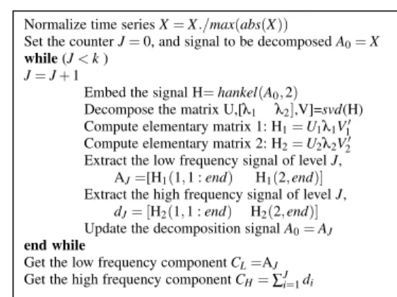
MSVD algorithm is summarized as the pseudo code shown in Figure 1. The input is the observed time seriesxof lengthN, and at the end, two additive and intrinsic components are obtained as outputs,cL and
cH, which represent the low frequency and the high
frequency component respectively, each one of length
N. MSVD is performed in three steps, embedding
through a Hankel matrix of 2×(N−1)dimension as 27, decomposition in orthogonal matrices of eigen-vectors U and V, and singular values λ1,λ2; finally unembedding from elementary matrices H1 and H2.
MSVD is processed iteratively and it is controlled by
J until the k repetition is done. When the singular spectrum rate ∆Rreaches the asymptotic point the k
value is set. The computation of∆Ris made by means of the next equations:
∆Rj= Rj Rj−1 (26a) Rj= λ1,j λ1,j+λ2,j (26b) whereRjis the Relative Energy of the singular values,
and j=1,2.
The Hankel matrix has the form:
H= x1 x2 . . . xN−1 x2 x2+1 . . . xN . (27)
The Hankel matrixHin all repetitions will have 2×K
dimension.
4.
C
ASES
TUDY 4.1. DataThree relevant nonstationary time series of traf-fic accidents are used, the data were collected by the Chilean police and the National Traffic Safety Commission (CONASET) from year 2000 to 2014 in Santiago de Chile with 783 weekly registers. This problem has socioeconomic relevance in planning and management; besides forecasting based on the prin-cipal improper behavior of drivers, passengers, and
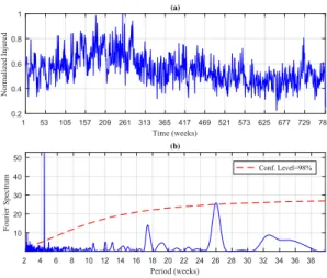
pedestrians will contribute highly in prevention tasks. CONASET has defined one hundred causes of traffic accidents. In this study case are used the time series of Injured-G1, which involves 10 main causes of traffic accidents related with improper behavior of drivers, passengers, and pedestrians. Detailed information was shown in Table 1. The full thesis shows the complete analysis of other groups obtained with the regarding causes. Figure 2(a) shows the observed time series Injured-G1, whereas Figure 2(b) show the Fourier Power Spectrum (FPS). The FPS analysis shown the signal spectrum and the red noise spectrum. Injured-G1 presents the highest peak at week 26 at 98 % of confidence level. With the peaks information the AR order is set asP=26.
4.2. Decomposition based on HSVD and compared with Singular Spectrum Analysis
Both preprocessing techniques HSVD and SSA embed the time series in a trajectory matrix. The initial window length used isL=N/2, based on theNlenght of the series. The embedding matrix H is then de-composed in singular values and singular vectors. The differential energy of the singular values is obtained with 25.
In this case, a high energy content was observed in the first t =20 eigenvalues. The lowest peaks of differential energy was used and evaluated to set the effective window length. Some experiments were developed examining diverse effective window length values, finally it was chosen by trial and error from those energy peaks that were given by the differential energy of the singular values. Then the effective win-dow length was set inL=15,L=17, andL=15, for Injured-G1, Injured-G2, and Injured-G3 respectively. The embedding process is implemented again with the effective window L, and the decomposition is recomputed following the methodology.
The first elementary matrixH1 is computed and it is
used to obtain the low frequencyCL component. In
HSVD direct extraction (unembedding) is performed from the first row and last column ofH1. While in SSA,
diagonal averaging is computed overH1. Finally the
component of high frequency is computed by simple difference.
The components extracted by HSVD and SSA are shown in Figure 3. TheCL components extracted by
HSVD and SSA from all signals are shown in Figure 3a. Long-memory periodicity features were observed in theCLcomponent. The resultant component of high
frequency is shown in Figure 3b, short-term periodic fluctuations were identified in theCHcomponent.
Injured-G1 signals show that the principal 10 causes present the highest incidence between years 2002 to 2005 (weeks 106 to 312), it descends from 2006 until half 2012 (around week 710), an increment is observed between weeks 711 and 732 (second semester of 2013 and first semester of 2014).
Prevention plans and punitive laws have been imple-mented in Chile during the analyzed period, vial edu-cation, drivers licensing reforms, zero tolerance law, Emilia’s law, transit law reforms, among others. The effect of a particular preventive or punitive action is not analyzed in this application, however the proposed short-term prediction methodology based on observed causes and intrinsic components is a contribution to government and society in preventive plans formula-tion, its implementation and the consequent evaluation.
4.3. Decomposition based on MSVD and compared with Wavelet Decomposition
MSVD implements an hierarchical process which finish when ∆R reaches the asymptotic value. The Singular Spectrum Rate ∆R for each decomposition level J are illustrated in Fig. 4, the asymptotic value is reached when∆R≈1, and it was observed in the repetition 16. Therefore the iterative process finish when iteration 16 was performed, this condition is used with all time series. The Wavelet Decomposition is based on Stationary Wavelet Transform (SWT). The decomposition is implemented through the function Daubechies of order 2 (Db2) (due to the inaccu-rate results that were obtained with the other type of wavelet functions they are not presented). Three decomposition levels (J=3) were selected according with the period fluctuation between 8 and 16 weeks. Figure 5 shows the components of low frequency and high frequency obtained with MSVD and SWT. The
cL components extracted by both MSVD and SWT,
show long-memory periodicity features, whereas the
4.4. Prediction through HSVD-AR, SSA-AR, HSVD-ANN, SSA-ANN
Before prediction, each data set of low and high frequency has been divided into two subsets, training and testing; the training subset involves 70 % of the samples, and consequently the testing subset involves the remaining 30 %. Multi-step ahead forecasting was implemented by means of multiple models in reason that direct strategy is used. The forecasting accu-racy is measured with normalized Root Mean Square Error (nRMSE) and modified Nash-Sutcliffe Efficiency (mNSE). The results are presented in Table 2. The results shows that the accuracy decreases as the time horizon increases. The best accuracy was reached by using SSA-AR for 1 to 10-week ahead forecasting while for 11 to 14-week ahead forecasting HSVD-AR is more accurate. SSA-AR present an averagenRMSE
of 0.013 and an averagemNSEof 92.7 %, it is followed by HSVD-AR with an averagenRMSE of 0.019 and an averagemNSEof 89.2 %. The lowest accuracy was reached by HSVD-ANN with an averagenRMSE of 0.047 and an averagemNSE of 72.7 %. Those blank spaces corresponds to poor results that were obtained.
4.5. Prediction through MSVD-MIMO and SWT-MIMO
The MIMO model is implemented to predict the number of injured people in traffic accidents for multiple horizon. The Autoregressive model is used with MIMO, the spectral analysis developed through FPS informs about the order of the model, it was shown in Figure 2b. The inputs of the AR model are thePlagged values ofcL and thePlagged values of
cH, and the outputs are the number of injured for the
nextτweeks. The prediction performance is evaluated with efficiency metrics nRMSE, mNSE, and mIA, which are presented in Table 3.
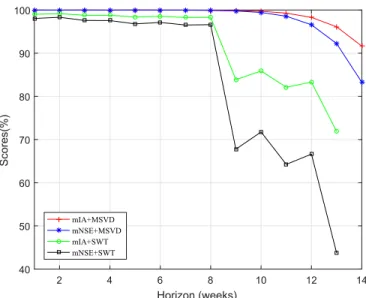
From Table 3 and Fig. 10, both models present good accuracy, however MSVD-MIMO model presents higher accuracy in comparison with SWT-MIMO. MSVD-MIMO obtains a significative gain in each forecasting horizon. The mean gain for 1 to 13 weeks of MSVD-MIMO over SWT-MIMO is 17.7 % in
mNSE and 8.1 % in mIA. SWT-MIMO results for 14-weeks ahead prediction are not presented due to the poor results that were obtained.
The Injured-G1 prediction via MSVD-MIMO for
14-weeks ahead prediction is shown in Figures 8a and 8b; from figures good fit is observed between actual and estimated values. Metrics computation give a nRMSE of 2.9 %, a mNSE of 83.3 % and a
mIA of 91.6 %. The prediction of the same series via SWT-MIMO for 13-weeks ahead prediction is shown in Fig. 9; lower accuracy is observed with anRMSE
of 10.1 %,amNSEof 43.7 % and amIAof 71.8 %. Various empirical applications were implemented to evaluate the proposed decomposition. Some time series of traffic accidents and other coming from fishe-ries domain.
5.
C
ONCLUSIONSThe main contribution of this research are new models for extracting components of low and high frequency from a nonstationary time series. Conven-tional linear and nonlinear models are reinforced with a potent preprocessing stage which achieves identif-ying spectral structures of an nonlinear and nonstatio-nary time series. Two type of spectral signals named components are extracted, one of low frequency and the other of high frequency. The components have the same length as the original signal but they have different magnitude and fluctuation. The component of low frequency represents long-memory periodicity features, whereas the components of high frequency represent short-term periodic fluctuations.
The proposed methods implemented in the preproces-sing stage are based on the Singular Value Decompo-sition of a Hankel matrix. Hankel is a matrix which is used to embed a discrete and univariate time series. New elementary matrices can be computed from the singular values and singular vectors obtained in the decomposition. Despite this transformation, the matri-ces structure gave us the assurance that the locations of the elements of the original data never be altered. This advantage allowed us the easy identification and extraction of the elements for each component from each elementary matrix. Nevertheless the difference of signals, they keep the original dynamics of the pheno-mena which is an important feature for prediction. The proposed methods were evaluated with nonsta-tionary time series of traffic accidents and fisheries domains. The data of traffic accidents consist of daily and weekly observations of quantities of accidents,
injury and deaths in three Chilean regions, Santiago, Valparaíso and Concepción, all covering the period January 1st 2000 to December 31th 2014. While the data of fisheries consist of monthly catches of anchovy, hake, sardine, and shrimp in some zones of pacific ocean coast, some of them covering the last five decades.
The decomposition method HSVD requires an unique parameter for its implementation, the window length (L). Unfortunately the finding of an effective window length could become frustrating. In this research, the selection of L is dependent of the singular values energy obtained with a initial window lengthL=N/2, where N is the sample size. The group of singular values with the largest energy concentration meant for us the way to obtain the best decomposition. Therefore the number of singular values with the largest relative energy concentration informs about the length of the effective window.
To avoid the limitation of HSVD due to the window length searching, a new decomposition method called MSVD was proposed. MSVD means Multilevel Singu-lar Value Decomposition of a Hankel matrix. MSVD is the iterative version of HSVD with a constant window lengthL=2. MSVD extracts the components of low and high frequency through a hierarchical process that decompose iteratively the component of low frequency whereas the component of high frequency is the resi-dual part. MSVD presents simplicity with respect to other techniques based on singular values by the use of a fixed window length in the embedding step, and although MSVD is iterative, the stoping condition is guarantee.
Singular Spectrum Analysis was also implemented with comparison purpose. SSA and HSVD implements the steps of embedding and decomposition, the diffe-rence among SSA and HSVD is in the step of compo-nents extraction. SSA implements diagonal averaging whereas HSVD implements unembedding, both from the correspondent elementary matrix.
One-step-ahead forecasting and multi-step ahead fo-recasting models were implemented to valid the pro-posed decomposition methods. Empirical applications shown high accuracy by means of all forecasting models based on HSVD and MSVD. Those models based on MSVD reaches the highest accuracy for one-step and multi-one-step ahead forecasting with an average
MAPE of 0.0011 % for one-week ahead forecasting
of Injured persons in traffic accidents and an avera-ge MAPE of 0.0053 for anchovy and sardine stock. Conventional ANN-based forecasting gave us low ac-curacies, for one-week ahead forecasting of Injured in traffic accidents it was obtained an average MAPE
of 4.1 %. Whereas for anchovy and sardine it was obtained an averageMAPEof 14.8 %
MSVD-MIMO is the result of the combination of data preprocessing and linear modelling. The model obeys three features: nonparametric, low complexity and reliability. These features guaranteeflexibilityfor stationary and nonstationary time series, easy imple-mentation and exactness by the use of a pure AR model, andreliability by the high accuracy obtained for multi-step ahead prediction.
MSVD-MIMO was also compared with the perfor-mance of the conventional wavelet decomposition. Stationary Wavelet Transform combined with MIMO (SWT-MIMO) was calibrated by means of the spectral information of the signal and by trial and error the Daubechies function was selected. Empirical appli-cations shown the superiority of MSVD-MIMO over SWT-MIMO. For 14-weeks ahead forecasting of Inju-red series, MSVD-MIMO reaches an average mNSE
of 97.7 %, whereas SWT-MIMO presents poor results. For 13-weeks ahead forecasting SWT-MIMO reaches an average mNSE of 82.6 %, and SSA-AR obtains an average mNSE of 92.9 %. On the other hand for 15-months ahead forecasting of anchovy and sardine stock, MSVD-MIMO reaches an average nNSE of 97.5 %, whereas SWT-MIMO presents 95.5 %, and SSA-AR an average mNSE of92.6 %. Furthermore MSVD presents simplicity with respect to SWT by the additional processing that is required by SWT to select the wavelet function, and with respect to SSA because it avoids the setting of an effective window length. About the contribution to the application domains, valuable information was identified. For traffic acci-dents, the ranking technique was applied to detect the relevant causes of injured people, it was observed the predominance of those causes related with improper behavior of drivers, pedestrians and passengers. Un-wise distance, Inattention to traffic conditions, and
Disrespect to red lightare the first important causes of injured people in traffic accidents in concordance with previous studies that determinedisrespect towards the road signsa principal cause of traffic accidents. Com-plementary information was observed about traffic
accidents conditions with high rate of injured people, automobiles type, environmental conditions, relative position, among others. About stock fisheries forecas-ting, the highest gain of MSVD-MIMO with respect to SWT-MIMO was observed for 12-months ahead prediction which is relevant for the annual fleet.
6.
F
UTUREW
ORKThe proposed models were evaluated in both do-mains, traffic accidents and fishing stock, however there is a large amount of information for future analysis. Traffic accidents with presence of deceased and injuries require more studies to support prevention plans of the government institutions. It is necessary to carry out new cross and deep analyzes related to circumstantial elements such as the condition of the road, atmospheric situation, relative position, vehicles involved, zone, among others. On the other hand, climate data captured by drones operating along Chile in real time, will provide more information for fore-casting in several productive areas such as the fishery industry.
The Mining Industry is an area of great socio-economic impact that can be researched through the proposed decomposition methods. It has been proven that through the study of mechanical vibrations, ano-malous signals can be observed in critical rotational machinery. Analysis in the frequency domain and arti-ficial intelligence have been commonly implemented to identify the spectral features of signals coming from vibrations. By means of our proposed methods a mechanical vibration could be decomposed into its endogenous components of low and high frequency, normal or anomalous, which coexist in the same signal and that are not clearly appreciable by conventional methods. Once the components are separated the fault is detected. With the anomalous components it is possible to diagnose the severity of the damage and the implementation of new forecasting models.
7.
A
CKNOWLEDGMENTSI want to thank principals of Pontificia Universidad Católica de Valparaíso by the scholarship that granted me. My special thanks to Vicerrectoría de Investiga-ción y Estudios Avanzados by the thesis term grant.
R
EFERENCIAS[1] Chatfield C., : The Analysis of Time Series: An Introduction, Sixth Edition. Taylor & Francis Group, LL. (2003) [2] Joo T. and Kim S.: Time series forecasting based on wavelet
filtering. Expert Systems with Applications. 42(8) 3868 -3874. (2015)
[3] Wayne A. Woodward and Henry L. Gray and Alan C. Elliott: Applied Time Series Analysis. Taylor & Francis Group. (2012)
[4] George E.P. Box and Gwilym M. Jenkins and Gregory C. Reinsel and Greta M. Ljung: Time Series Analysis: Forecas-ting and Control, fifth edition. Wiley & Sons. (2009) [5] Stewart G.: On the Early History of the Singular Value
Decomposition. SIAM Review, 35(4) 551 - 566. (1993) [6] R.E. Abdel-Aal and A.Z. Al-Garni: Forecasting monthly
electric energy consumption in eastern Saudi Arabia using univariate time-series analysis. Energy. 22(11) 1059 - 1069. (1997)
[7] Vaseghi S.: Advanced Digital Signal Processing and Noise Reduction Third Edition. Wilew & Sons. (2006)
[8] Narayanan P. and Basistha A. and Sarkar S., and Kamna S.: Trend analysis and ARIMA modelling of pre-monsoon rainfall data for western India. Comptes Rendus Geoscience. 345(1) 22 - 27. (2013)
[9] Hassan J.: ARIMA and regression models for prediction of daily and monthly clearness index. Renewable Energy. 68(0) 421 - 427. (2014)
[10] Cho V.: Tourist forecasting and its relationship with leading economic indicators. Journal of Hospitality and Tourism Research. 25(0) 399 - 420. (2001)
[11] Li G. and Shi J.: On comparing three artificial neural networks for wind speed forecasting. Applied Energy. 87(7) 2313 - 2320. (2010)
[12] Laboissiere L., Fernandes R., and Lage G.: Maximum and minimum stock price forecasting of Brazilian power distribution companies based on artificial neural networks. Applied Soft Computing. 35(0) 66 - 74. (2015)
[13] Vapnik V.: The Nature of Statistical Learning Theory. Springer - Verlag, 119 - 156. (1995)
[14] Levis A., Papageorgiou L.: Customer Demand Forecasting via Support Vector Regression Analysis. Chemical Enginee-ring Research and Design, 83(8) 1009 - 1018. (2005) [15] Abdollahzade M., Miranian A., Hassani H., Iranmanesh
H.: A new hybrid enhanced local linear neuro-fuzzy model based on the optimized singular spectrum analysis and its application for nonlinear and chaotic time series forecasting. Information Sciences, 295(0) 107 - 125. (2015)
[16] Grossmann A., Morlet J.: Decomposition of hardy fun-ctions into square integrable wavelets of constant shape. SIAM Journal on Mathematical Analysis, 15 (4) 723 - 736. (1984)
[17] Mallat S.: A Theory for Multiresolution Signal Decompo-sition: The Wavelet Representation. IEEE Transactions on pattern analysis and machine intelligence, 11 (7) 674 - 693. (1989)
[18] Daubechies I.: Orthonormal bases of compactly supported wavelets. Communications on Pure and Applied Mathema-tics, 41(7) 909 - 996. (1988)
[19] Seo Y., Kim S., Kisi O., Singh V.: Daily water level forecas-ting using wavelet decomposition and artificial intelligence techniques. Journal of Hydrology, 520 (0) 224 - 243. (2015) [20] Sun Y., Leng B., Guan W.: A novel wavelet-SVM short-time passenger flow prediction in Beijing subway system. Neurocomputing, 166 (0) 109 - 121. (2015)
[21] Bai Y., Li Y., Wang X., Xie J., Li C.: Air pollutants concentrations forecasting using back propagation neural network based on wavelet decomposition with meteorolo-gical conditions. Atmospheric Pollution Research, 7 (3) 557 - 566. (2016)
[22] Pektas A., Cigizoglu, K.: ANN hybrid model versus ARI-MA and ARIARI-MAX models of runoff coefficient. Journal of Hydrology, 500 (0)21 - 36. (2013)
[23] Fahmy A., El-Tantawy M., Gobran, Y.: Using artificial neural networks in the design of orthotropic bridge decks. Alexandria Engineering Journal. (2016)
[24] Wu Z., Huang N.: Ensemble empirical mode decompo-sition: a noise assisted data analysis method. Advances in Adaptive Data Analysis, 1(1) 1 - 41. (2009)
[25] Myung I.: Tutorial on maximum likelihood estimation. Journal of Mathematical Psychology, 47(1) 90 - 100. (2003) [26] Freeman J., Skapura D.: Neural Networks, Algorithms, Ap-plications, and Programming Techniques. Addison-Wesley. (1991)
[27] Golyandina N., Nekrutkin V., Zhigljavsky A.: Analysis of time series structure. Chapman & Hall/CRC. (2001)
[28] Lo ´eve M.: Sur les fonctions aleatoires stationnaires du
second ordre. Revue Scientifique. (83) 297 - 303 (1945) [29] Karhunen K. On the use of singular spectrum analysis for
forecasting U.S. trade before, during and after the 2008 recession. Annales Academiae Scientiarum Fennicae. (34) 1 - 7 (1946)
[30] Broomhead D. S., King G.P.: Extracting qualitative dyna-mics from experimental data. Physica D: Nonlinear Pheno-mena. 20(2), 217 - 236 (1986)
[31] Vautard R., Yiou P., Ghil M.: Singular-spectrum analysis: A toolkit for short, noisy chaotic signals. Physica D: Nonlinear Phenomena. 58(1) 95 - 126 (1992)
[32] Ghil M., Allen M.R.,Dettinger M.D., Ide K., Kondrashov D., Mann M.E., Robertson A.W., Saunders A., Tian Y., Varadi F., Yiou P.: Advanced Spectral Methods for Climatic Time Series. Reviews of Geophysics. 40(1) 3.1 - 3.41 (2002) [33] Kumar U., Jain V.K.: Time series models (Grey-Markov, Grey Model with rolling mechanism and singular spectrum analysis) to forecast energy consumption in India. Energy. 35(4) 1709 - 1716 (2010)
[34] Hassani H., Heravi S., Zhigljavsky A.: Forecasting Euro-pean industrial production with singular spectrum analysis. International Journal of Forecasting. 25(1) 103 - 118 (2009) [35] Hassani H., Webster A., Silva E., Heravi S.: Forecasting U.S. Tourist arrivals using optimal Singular Spectrum Analy-sis. Tourism Management. 46(0) 322 - 335 (2015) [36] Silva E.S. Hassani H.: On the use of singular spectrum
analysis for forecasting U.S. trade before, during and after the 2008 recession. International Economics. 141(0) 34 - 49 (2015)
[37] Comisión Nacional de Seguridad de Tránsito.
http://www.conaset.cl (2015)
[38] Secretaría Nacional de Pesca. http://www.sernapesca.cl (2015)
[39] Stewart G.: On the Early History of the Singular Value Decomposition. SIAM Review, 35 (4) 551 - 566. (1993) [40] Golub G., Van Loan C.: Matrix Computations, third edition.
The Johns Hopkins University Press. 257 -258 (1996) [41] Beck J., Arnold K.: Parameter Estimation in Engineering
and science. John Wiley & Sons. (1934)
Lida BarbaLida Barba is a pro-fessor at Engineering Faculty at Universidad Nacional de Chim-borazo (Ecuador). Lida reached her Doctors degree at Pontifi-cia Universidad Católica de Val-paraíso (Chile) in March, 2017; and her undergraduate studies at Escuela Superior Politécnica de Chimborazo (Ecuador). She is leader of research projects related to time series forecasting and data analysis with the use of mathematical, artificial intelligence, and hybrid based models.
Normalize time seriesX=X./max(abs(X))
Set the counterJ=0, and signal to be decomposedA0=X while(J<k)
J=J+1
Embed the signal H=hankel(A0,2)
Decompose the matrix U,[λ1 λ2],V]=svd(H) Compute elementary matrix 1: H1=U1λ1V10
Compute elementary matrix 2: H2=U2λ2V20
Extract the low frequency signal of levelJ, AJ=[H1(1,1 :end) H1(2,end)]
Extract the high frequency signal of levelJ,
dJ= [H2(1,1 :end) H2(2,end)]
Update the decomposition signalA0=AJ
end while
Get the low frequency componentCL=AJ
Get the high frequency componentCH=∑Ji=1di
1 53 105 157 209 261 313 365 417 469 521 573 625 677 729 783 Time (weeks) 0.2 0.4 0.6 0.8 1 Normalized Injured (a) 2 4 6 8 10 12 14 16 18 20 22 24 26 28 30 32 34 36 38 Period (weeks) 10 20 30 40 50 Fourier Spectrum (b) Conf. Level=98%
Figura 2. (a) Injured-G1, (b) FPS of Injured-G1. The thick solid line is the global wavelet spectrum for Injured-G1, while the dashed line is the red-noise spectrum
Time (weeks) 1 53 105 157 209 261 313 365 417 469 521 573 625 677 729 783 Innjured-G1 (norm.) 0.4 0.5 0.6 0.7 0.8 (a)
HSVD:Low Freq. SSA: Low Freq.
Time (weeks) 1 53 105 157 209 261 313 365 417 469 521 573 625 677 729 783 Injured-G1 (norm.) -0.2 -0.1 0 0.1 0.2 0.3 0.4 0.5 (b)
HSVD:High Freq. SSA: High Freq.
Figura 3. Injured-G1 components (a) Low frequency com-ponents via HSVD and SSA (b) High frequency compo-nents via HSVD and SSA
1 6 11 16 21 26 J-Level SVD 92 93 94 95 96 97 98 99 100 ∆ R (%) Injured-G1 Injured-G2 Injured-G3
Figura 4. Decomposition Levels vs Singular Spectrum Rate
1 53 105 157 209 261 313 365 417 469 521 573 625 677 729 783 Time (weeks) -0.4 -0.2 0 0.2 0.4 0.6 0.8 1 Normalized Injured MSVD: Low Freq SWT : Low Freq MSVD: High Freq SWT : High Freq
Figura 5. Injured-G1, Low Frequency Component and High Frequency Component via MSVD and SWT
horizon (weeks) 1 2 3 4 5 6 7 8 9 10 11 12 13 14 nRMSE 0 0.01 0.02 0.03 0.04 0.05 0.06 0.07 0.08 HSVD-AR SSA-AR HSVD-ANN SSA-ANN
Figura 6. nRMSE Results for multi-week ahead forecasting of Injured-G1 horizon (weeks) 1 2 3 4 5 6 7 8 9 10 11 12 13 14 mNSE (%) 50 53 56 59 62 65 68 71 74 77 80 83 86 89 92 95 98 100 HSVD-AR SSA-AR HSVD-ANN SSA-ANN
Figura 7. mNSE Results for multi-week ahead forecasting of Injured-G1
1 20 39 58 77 96 115 134 153 172 191 210 223 Time (weeks) 0.2 0.4 0.6 0.8 1 Normalized Injured (a) Actual Value Estimated Value 0.2 0.3 0.4 0.5 0.6 0.7 0.8 Target X 0.2 0.4 0.6 0.8 Y: Linear Fit (b) y=0.98816x+0.0060008 Data Points Best Linear Fit Y=X
Figura 8. Injured-G1 Prediction by MSVD-MIMO (a) Observed vs Predicted, (b) Linear Fit
1 20 39 58 77 96 115 134 153 172 191 210 223 Time (weeks) 0.2 0.4 0.6 0.8 1 Normalized Injured (a) Actual Value Estimated Value 0.2 0.3 0.4 0.5 0.6 0.7 0.8 Target X 0.2 0.4 0.6 0.8 Y: Linear Fit (b) y=0.68838x+0.14788 Data Points Best Linear Fit Y=X
2 4 6 8 10 12 14 Horizon (weeks) 40 50 60 70 80 90 100 Scores(%) mIA+MSVD mNSE+MSVD mIA+SWT mNSE+SWT
Figura 10. Multi-step forecasting results, comparison for Injured-G1
Cuadro 1
Causes of Injured in Traffic Accidents, Group 1 and Group 2
Category Num Cause Importance imprudent driving
1 Unwise distance 1 2 Inattention to traffic conditions 2 3 Disrespect to pedestrian passing 8 4 Disrespect for give the right of way 9 5 Unexpected change of track 10 6 Improper turns 11 7 Overtaking without enough time or space 14 8 Opposite direction 18 9 Backward driving 19 disobedience to signal
10 Disrespect to red light 3 11 Disrespect to stop sign 4 12 Disrespect to give way sign 6 13 Improper speed 13 alcohol in driver
14 Drunk driver 7 15 Driving under the influence of alcohol 15 recklessness in pedestrian
16 Pedestrian crossing the road suddenly 5 17 Reckless pedestrian 12 18 Pedestrian outside the allowed crossing 17 recklessness in passenger
19 Get in or get out of a moving vehicle 16 alcohol in pedestrian
Cuadro 2
Multi-step ahead forecasting results for Injured-G1 via Direct Strategy
nRMSE mNSE( %)
h(week) HSVD-AR SSA-AR HSVD-ANN SSA-ANN HSVD-AR SSA-AR HSVD-ANN SSA-ANN 1 0.008 0.001 0.01 0.002 95.7 99.3 93.7 99.1 2 0.011 0.003 0.02 0.003 93.6 98.4 89.4 97.8 3 0.015 0.005 0.03 0.007 91.7 97.4 83.0 96.5 4 0.018 0.007 0.04 0.011 90.1 96.3 79.0 93.8 5 0.020 0.009 0.04 0.014 89.0 95.0 78.8 91.6 6 0.021 0.011 0.04 0.018 88.1 93.6 75.0 88.4 7 0.023 0.014 0.06 0.027 87.0 92.1 67.0 87.1 8 0.024 0.017 0.06 0.036 86.8 90.7 64.4 79.3 9 0.024 0.019 0.07 0.041 86.9 89.3 62.0 75.6 10 0.024 0.022 0.07 0.056 86.8 87.9 61.9 73.5 11 0.023 0.024 0.07 0.056 87.1 86.7 61.5 70.7 12 0.022 0.026 0.07 0.060 87.7 85.6 56.5 67.8 13 0.020 0.028 0.07 - 89.1 84.9 57.7 -14 0.016 - 0.06 - 91.0 - - -min 0.008 0.001 0.011 0.002 86.8 84.9 56.5 67.8 max 0.024 0.028 0.074 0.06 95.7 99.3 93.7 99.1 mean 1-13 0.19 0.013 0.047 0.028 89.2 92.7 72.7 85.1 Cuadro 3
Multi-step MIMO forecasting results,nRMSE,mNSE, andmIAfor Injured-G1
RMSE mNSE( %) mIA( %) h(week) MSVD SWT MSVD SWT MSVD SWT
MIMO MIMO MIMO MIMO MIMO MIMO 1 0.0021 0.34 99.9 98.0 99.9 99.0 2 0.0030 0.29 99.9 98.3 99.9 99.2 3 0.0007 0.44 99.9 97.6 99.9 98.8 4 0.0030 0.44 99.9 97.6 99.9 98.8 5 0.0003 0.56 99.9 96.8 99.9 98.4 6 0.0024 0.51 99.9 97.1 99.9 98.6 7 0.0041 0.63 99.9 96.5 99.9 98.3 8 0.0125 0.61 99.9 96.6 99.9 98.3 9 0.0366 5.6 99.8 67.8 99.9 83.9 10 0.0990 4.8 99.4 71.6 99.7 85.9 11 0.2512 6.5 98.5 64.2 99.3 82.1 12 0.6009 5.9 96.6 66.6 98.3 83.3 13 1.3685 10.13 92.2 43.7 96.1 71.8 14 2.9872 - 83.3 - 91.6 -Min 0.0003 0.29 83.3 43.7 91.6 71.8 Max 2.9872 10.1 99.9 98.3 99.9 99.2 Mean 1-13 step 0.1834 2.8 98.9 84.1 98.9 92.0 Mean 1-14 step 0.3837 - 97.8 - 98.9