Macroeconomic forecasting and structural change

(1)

Working PaPer SerieS

no 1167 / aPriL 2010

MacroeconoMic

ForecaSting

and StructuraL

change

(2)

W O R K I N G PA P E R S E R I E S

N O 1167 / A P R I L 2 010

In 2010 all ECB publications feature a motif taken from the €500 banknote.

MACROECONOMIC FORECASTING

AND STRUCTURAL CHANGE

1

by Antonello D’Agostino

2

_{, Luca Gambetti}

3

and Domenico Giannone

4

NOTE: This Working Paper should not be reported as representing the views of the European Central Bank (ECB). The views expressed are those of the authors and do not necessarily reflect those of the ECB.

(3)

© European Central Bank, 2010 Address

Kaiserstrasse 29

60311 Frankfurt am Main, Germany

Postal address

Postfach 16 03 19

60066 Frankfurt am Main, Germany

Telephone +49 69 1344 0 Internet http://www.ecb.europa.eu Fax +49 69 1344 6000

Any reproduction, publication and reprint in the form of a different publication, whether printed or produced electronically, in whole or in part, is

(4)

Abstract 4

Non-technical summary 5

1 Introduction 7

2 The time-varying vector autoregressive model 10

2.1 Forecasts 11

2.2 Priors specifi cation 12

3 Real-time forecasting 13

3.1 Data 13

3.2 How much time variation? 14

3.3 Other forecasting models 15

3.4 Forecast evaluation 16

4 Results 16

5 Conclusions 19

References 20

Appendix 22

Tables and fi gures 26

(5)

Abstract

The aim of this paper is to assess whether explicitly modeling structural change increases the ac-curacy of macroeconomic forecasts. We produce real time out-of-sample forecasts for inflation, the unemployment rate and the interest rate using a Time-Varying Coefficients VAR with Stochastic Volatility (TV-VAR) for the US. The model generates accurate predictions for the three variables. In particular for inflation the TV-VAR outperforms, in terms of mean square forecast error, all the competing models: fixed coefficients VARs, Time-Varying ARs and the na¨ıve random walk model. These results are also shown to hold over the most recent period in which it has been hard to forecast inflation.

JEL classiﬁcation: C32, E37, E47.

Keywords: Forecasting, Inﬂation, Stochastic Volatility, Time Varying Vector Autoregres-sion.

(6)

Non technical summary

The aim of this paper is to assess whether explicitly modelling structural change increases the accuracy of macroeconomic forecasts. In principle, allowing for structural changes may improve the forecast performance for at least two reasons. First, it allows capturing and exploiting changes in macroeconomic relationships. Second, empirical models that allow for structural changes can correctly detect and forecast changes in the long run dynamics, like the decline in trend inflation and unemployment observed since the mid 80s; however, a richer model structure can worsen the forecasting performance. A higher number of parameters increases the estimation errors, which in turn can affect the forecast accuracy. The model we use in this paper is sufficiently general and flexible. We allow for both changes in the coefficients and in the volatility. In particular, we use the Time-Varying Coefficients VAR with Stochastic Volatility (TV-VAR). The model allows for a) changes in the predictable component (time-varying coefficients), which can be due to variations in the structural dynamic interrelations among macroeconomic variables; and b) changes in the unpredictable component (stochastic volatility), that is, variations in the size and correlation among forecast errors, which can be due to changes in the size of exogenous shocks or their impact on macroeconomic variables.

We forecast three macroeconomic variables for the US economy: the unemployment rate, inflation and a short term interest rate. We aim to mimic as close as possible the conditions faced by a forecaster in real-time. We use “real-time data” to compute predictions based only on the data that were available at the time the forecasts are made. The accuracy of the predictions (the mean square forecast errors) of the TV-VAR is compared to the accuracy of other standard forecasting models: fixed coefficients VARs (estimated recursively or with rolling window), Time-Varying ARs and the naive random walk model.

Our findings show that the TV-VAR is the only model which systematically delivers accurate forecasts for the three variables. Inflation predictions at long horizons produced by the TV-VAR are much more accurate than those obtained with any other model. These results hold for the Great Moderation period (after mid 1980's). This is particularly

(7)

Forecasting evaluation has important implications even if the ultimate goal is not forecasting. It is a powerful validation procedure which is particularly important for very flexible and general models such as the TV-VAR. In general, introducing complexity in the model to better describe the data does not necessary enhance real-time forecasting performances. The benefit from more flexibility might be limited if the more flexibility captures also non prominent features of the data. If model complexity is introduced with a proliferation of parameters, instabilities due to estimation uncertainty might completely offset the gains obtained by limiting model miss-specification. Our results indicate that the TV-VAR model is a very powerful tool for real-time forecasting since it incorporates in a flexible but parsimonious manner the prominent features of a time-varying economy.

(8)

1 Introduction

The US economy has undergone many structural changes during the post-WWII period. Long run trends in many macro variables have changed. Average unemployment and infla-tion were particularly high during the 70s and low in the last decades (see Staiger, Stock, and Watson, 2001). Business cycle fluctuations have moderated substantially in the last twenty years and the volatility of output growth has reduced sharply. This latter phe-nomenon is typically referred to as the ”Great Moderation” (Stock and Watson, 2004). Also the dynamics of inflation have changed drastically: after the mid 80s inflation has become more stable and less persistent (see Cogley and Sargent, 2001).1

In addition to these series-specific changes many important changes in the relationships between macroeconomic variables have been documented. For instance, some authors have argued that the Phillips curve is no longer a good characterization of the joint dynamics of inflation and unemployment. Such a claim is partly based on the result that the predictive content of unemployment for inflation has vanished since the mid 80s (Atkeson and Ohanian, 2001; Roberts, 2006; Stock and Watson, 2008a).2 The same period has seen significant changes in the conduct of macroeconomic policy. For example, according to many observers, monetary policy has become much more transparent and aggressive against inflation since the early 80s (Clarida, Gali, and Gertler, 2000).

In this paper we address the following question: can the accuracy of macroeconomic forecasts be improved by explicitly modeling structural change? The answer to this question is far from trivial. On the one hand, clearly, if the economy has changed, a forecasting model that can account for such changes would be better suited and should deliver better forecasts. On the other hand, however, a richer model structure implying a higher number of parameters should increase the estimation errors and reduce the forecast accuracy.

The relevance of modeling time variation was originally stressed by Doan, Litterman,

1_{Changes in persistence are still debated, for instance Pivetta and Reis (2007) ﬁnd that the changes are} not signiﬁcant.

2_{More generally, the ability to exploit macroeconomic linkages for predicting inﬂation and real activity} seems to have declined remarkably since the mid-1980s, see (D’Agostino, Giannone, and Surico, 2006) and Rossi and Sekhposyan (2008).

(9)

and Sims (1984), but surprisingly there are only a few studies aiming at exploring the issue systematically (see Stock and Watson (1996), Canova (2007), Clark and McCracken (2007), Stock and Watson (2007)). These studies use diﬀerent models and forecasting periods but they all share a common feature: they focus on the time variation in the coeﬃcients but do not allow for changes in volatility. The only exception is Stock and Watson (2007) who, however, do not have lagged dynamics in their forecasting equation.

We forecast three macroeconomic variables for the US economy, the unemployment rate, inflation and a short term interest rate, using a Time-Varying Coefficients VAR with Stochastic Volatility (TV-VAR henceforth) as specified by Primiceri (2005). The model is very flexible. In particular it allows for a) changes in the predictable component (time-varying coefficients), which can be due to variations in the structural dynamic interrelations among macroeconomic variables; and b) changes in the unpredictable component (stochastic volatility), that is, variations in the size and correlation among forecast errors, which can be due to changes in the size of exogenous shocks or their impact on macroeconomic variables.3 In the forecasting exercise we aim at mimicking as close as possible the conditions faced by a forecaster in real-time. We use “real-time data” to compute predictions based only on the data that were available at the time the forecasts are made. We forecast up to 3 years ahead. This longer horizon has been chosen to fill the gap with the existing literature, which has mainly focused on the shorter horizons up to one year.4 Long run persistent components can play a crucial role in explaining longer horizon dynamics, while their contribution in explaining short run movements in the variables can be negligible.

The accuracy of the predictions (the mean square forecast errors) of the TV-VAR are compared to the predictions based on other standard forecasting models: ﬁxed coeﬃcients VARs (estimated recursively or with rolling window), Time-Varying ARs and the na¨ıve random walk model.

The assessment of the forecasting performance of econometric models has become

stan-3_{Allowing for the two sources of change is also important in the light of the ongoing debate about the} relative importance of changes in the predictable and unpredictable components in the Great Moderation (Giannone, Lenza, and Reichlin, 2008).

(10)

dard in macroeconomics, even if the ultimate goal is not forecasting. Forecasting evaluation can be seen as a validation procedure which is particularly important for very flexible and general models. In general, introducing complexity in the model to better describe the data does not necessary enhance real-time forecasting performances. The benefit from more flex-ibility might be limited if the more flexflex-ibility captures also non prominent features of the data. If model complexity is introduced with a proliferation of parameters, instabilities due to estimation uncertainty might completely offset the gains obtained by limiting model miss-specification. Out-of-sample forecasting evaluations represent hence an important device to evaluate the ability of capturing prominent features of the data within a parsimonious mod-els. In addition, the out-of-sample exercise will also provide indications on some subjective choices that are required for the estimation of the TV-VAR model, such as the setting of the prior beliefs on the relative amount of time variations in the coefficients.

In addition, the paper studies another core aspect of the TV-VAR model which has not been tackled by the previous literature; the effect of explosive roots on the forecast accuracy. In particular, we compare the predictive ability of the model in two cases: in the first one the explosive paths (draws which make instable the system) are excluded, while in the second one such restriction is not imposed and all draws are used to compute the forecasts. The presence of explosive paths could have relevant effects especially over the longer horizon forecasts.5

Our main findings show that the TV-VAR is the only model which systematically de-livers accurate forecasts for the three variables. For inflation the forecasts generated by the TV-VAR are much more accurate than those obtained with any other model. For unem-ployment, the forecasting accuracy of the TV-VAR model is very similar to that of the fixed coefficient VAR, while forecasts for the interest rate are comparable to those obtained with the Time-Varying AR. These results hold for different sub-samples. In particular, they are also confirmed over the Great Moderation period, a period in which forecasting models are often found to have difficulties in outperforming simple na¨ıve models in forecasting many macroeconomic variables especially inflation. Results suggest that, on the one hand time

5_{Clark and McCracken (2007) found that the time-varying VAR performs particularly badly over the ten} year horizon. This might be due to the presence of explosive roots.

(11)

varying models are “quicker” in recognizing structural changes in the permanent compo-nents of inﬂation and interest rate, and, on the other hand, that short term relationships among macroeconomic variables carry out important information, once structural changes are properly taken into account.

The rest of the paper is organized as follows, section 2 describes the TV-VAR model; section 3 explains the forecasting exercise; section 4 presents the results and section 5 concludes.

2 The Time-Varying Vector Autoregressive Model

Lety_t= (π_t, U R_t, IR_t) whereπ_tis the inﬂation rate,U R_t the unemployment rate andIR_t

a short term interest rate. We assume thaty_tadmits the following time varying coeﬃcients VAR representation:

y_t=A₀_,t+A₁_,ty_t₋₁+...+A_p,ty_t₋_p+ε_t (1)

where A₀_,t contains time-varying intercepts, A_i,t are matrices of time-varying coeﬃcients,

i = 1, ..., p and ε_t is a Gaussian white noise with zero mean and time-varying covariance

matrix Σ_t. LetA_t= [A₀_,t, A₁_,t..., A_p,t], andθ_t=vec(A_t),wherevec(·) is the column stacking operator. Conditional on such an assumption, we postulate the following law of motion for

θ_t:

θ_t=θ_t₋₁+ω_t (2)

whereω_t is a Gaussian white noise with zero mean and covariance Ω. We let Σ_t=F_tD_tF_t, whereF_tis lower triangular, with ones on the main diagonal, andD_ta diagonal matrix. Let

σ_t be the vector of the diagonal elements ofD_t1/2 andφ_i,t,i= 1, ..., n−1 the column vector formed by the non-zero and non-one elements of the (i+ 1)-th row ofF_t−1. We assume that the standard deviations,σ_t, evolve as geometric random walks. The simultaneous relations

φ_it in each equation of the VAR are assumed to evolve as independent random walks.

logσ_t= logσ_t₋₁+ξ_t (3)

(12)

where ξ_t and ψ_i,t are Gaussian white noises with zero mean and covariance matrix Ξ and Ψ_i, respectively. Let φ_t= [φ₁_,t, . . . , φ_n₋₁_,t], ψ_t= [ψ₁_,t, . . . , ψ_n₋₁_,t], and Ψ be the covariance matrix ofψ_t. We assume thatψ_i,t is independent of ψ_j,t, for j=i, and that ξ_t,ψ_t, ω_t, ε_t

are mutually uncorrelated at all leads and lags.6

2.1 Forecasts

Equation (1) has the following companion form

yt=μt+Atyt−1+t

whereyt= [yt...yt−p+1],t= [εt0...0] andμt= [A₀,t0...0] arenp×1 vectors and

At=

A_t

I_n₍_p₋₁₎ 0_n₍_p₋₁₎_,n

whereA_t= [A₁_,t...A_p,t] is ann×npmatrix, I_n₍_p₋₁₎ is ann(p−1)×n(p−1) identity matrix and 0_n₍_p₋₁₎_,n is an(p−1)×nmatrix of zeros. Let ˆμ_tand ˆA_t denote the median of the joint posterior distribution ofμ_t A_t (see appendix for the details). The one-step ahead forecast is

ˆ

yt+1|t= ˆμt+ ˆAtyt (5)

A technical issue arises when we generate multi-step expectations; we have to evaluate the future path of drifting parameters. We follow the literature and treat those parameters as if they had remained constant at the current level.7 As a consequence, forecasts at time

t+hare computed iteratively:

ˆ yt+h|t= ˆμt+ ˆAtyˆt+h−1 = h j=1 ˆ Aj−1 t μˆt+ ˆAhtyt (6)

6_{In principle, one could make} _ε

t and ωt correlated. However, it is well known that such model can be

equivalently represented with a setup where shocks are mutually uncorrelated butεt is serially correlated. Since our measurement equation is a VAR, such a ﬂexibility is unnecessary here.

(13)

2.2 Priors speciﬁcation

The model is estimated using Bayesian methods. While the details of the estimation are accurately described in the Appendix, in this section we briefly discuss the specification of our priors. Following Primiceri (2005), we make the following assumptions for the priors densities. First, the coefficients of the covariances of the log volatilities and the hyperpa-rameters are assumed to be independent of each other. The priors for the initial states θ₀,

φ₀ and logσ are assumed to be normally distributed. The priors for the hyperparameters, Ω, Ξ and Ψ are assumed to be distributed as independent inverse-Wishart. More precisely, we have the following priors:

• Time varying coeﬃcients: P(θ₀) =N(ˆθ,Vˆ_θ) and P(Ω) =IW(Ω−₀1, ρ₁);

• Stochastic Volatilities: P(logσ₀) =N(log ˆσ, I_n) and P(Ψ_i) =IW(Ψ−₀_i1, ρ₃_i);

• Simultaneous relations: P(φi0) =N( ˆφi,Vˆφi) andP(Ξ) =IW(Ξ−01, ρ2);

where the scale matrices are parameterized as follows Ω−₀1 =λ₁ρ₁Vˆ_θ, Ψ₀_i =λ₃_iρ₃_iVˆ_φ_i and Ξ₀ = λ₂ρ₂I_n. The hyper-parameters are calibrated using a time invariant recursive VAR estimated using a sub-sample consisting of the ﬁrst T₀ observations.8 For the initial states

θ₀and the contemporaneous relationsφ_i₀, we set the means, ˆθand ˆφ_i, and the variances, ˆV_θ

and ˆV_φ_i, to be the maximum likelihood point estimates and four times its variance. For the initial states of the log volatilities, logσ₀, the mean of the distribution is chosen to be the logarithm of the point estimates of the standard errors of the residuals of the estimated time invariant VAR. The degrees of freedom for the covariance matrix of the drifting coeﬃcient’s innovations are set to be equal toT₀, the size of the initial-sample. The degrees of freedom for the priors on the covariance of the stochastic volatilities’ innovations, are set to be equal to the minimum necessary for insuring the prior is proper. In particular, ρ₁ and ρ₂ are equal to the number of rows Ξ−₀1 and Ψ−₀_i1 plus one respectively. The parameters λ_i are very important since they control the degree of time variations in the unobserved states. The smaller such parameters are, the smoother and smaller are the changes in coeﬃcients. The empirical literature has set the prior to be rather conservative in terms of the amount

8_T

(14)

of time variations. The exact parameterizations used will be discussed in the empirical section.

3 Real-time forecasting

Our objective is to predict the h-period ahead unemployment rate U R_t₊_h, the interest rateIR_t₊_h and the annualized price inﬂationπh_t₊_h = 400_h log(P_Pt+h

t ), where Pt+h is the GDP

deﬂator at timet+h and 400_h is the normalization term.

3.1 Data

Prices are measured by the GDP deflator and the interest rate is measured by the three month treasury bills. We use real time data forP_tandU R_t,9 while the three month interest rate series is not subject to revisions.10 Since unemployment and interest rate series are available at monthly frequency, we follow Cogley and Sargent (2001, 2005) and Cogley, Primiceri, and Sargent (2008) and convert them into quarterly series by taking the value at the mid-month of the quarter forU R_tand the value at the first month of the quarter forIR_t. We use quarterly vintages from 1969:Q4 to 2007:Q4. Vintages can differ since new data on the most recent period are released, but also because old data get revised. As a convention we date a vintage as the last quarter for which all data are available. For each vintage the sample starts in 1948:Q1.11 For the GDP deflator we compute the annualized quarterly inflation rate, π_t= 400 log( Pt

Pt−1). We perform an out-of-sample simulation exercise.12 The

procedure consists of generating the forecasts by using the same information that would have been available to the econometrician who had produced the forecasts in real time. The simulation exercise begins in 1969:Q4 and, for such a vintage, parameters are estimated

9_The _data _are _available _on _the _Federal _Reserve _Bank _of _Philadelphia _website _at:

http://www.phil.frb.org/econ/forecast/reaindex.html.

10_{The series is available on the FRED dataset of the Federal Reserve Bank of St. Louis (mnemonics} TB3MS), at: http://research.stlouisfed.org/fred2/series/TB3MS

11_{The vintages have a diﬀerent time length, for example the sample span for the ﬁrst vintage is} 1948:Q1-1969:Q4, while the sample span for the last available vintage is 1948:Q1-2007:Q4.

12_{Data for the same period can diﬀer across vintages because of revisions; for notational simplicity we} drop the indication of the vintage.

(15)

using the sample 1948:Q1 to 1969:Q4. The model is estimated with two lags. We compute the forecasts up to 12 quarters ahead outside the estimation window, from 1970:Q1 to 1972:Q4, and the results are stored.13 Then, we move one quarter ahead and re-estimate the model using the data in vintage 1970:Q1. Forecasts from 1970:Q2 to 1973:Q1 are again computed and stored. This procedure is then repeated using all the available vintages. Predictions are compared with ex-post realized data vintages. Since data are continuously revised at each quarter, several vintages are available. Following Romer and Romer (2000), predictions are compared with the figures published after the next two subsequent quarters. These figures are conceptually similar to the series being predicted in real time since they do not incorporate rebenchmarking and other definitional changes. In addition, these figures are based on a relatively complete set of data available to the statistical offices. Qualitative results are confirmed if we compare with final data.

Two important aspects of the TV-VAR specification are worth noting. The first one concerns the setting of λ_i, the parameter which fixes the tightness of the variance of the coefficients . In general, the literature has been quite conservative; very little time variation has been used in practice to set this parameter. The second aspect concerns the inclusion (or exclusion) of explosive draws from the analysis. That is, whether to keep or discard draws whose (VAR polynomial) roots lie inside the unit circle. We report results for the most conservative priors of Primiceri (2005) (λ₁ = (0.01)2, λ₂ = (0.1)2 and λ₃ = (0.01)2) and discard the explosive draws. However, we also run some robustness checks to understand the sensitivity of the model to alternative specifications. In a first simulation, we set more stringent priors, while in a second simulation we keep the explosive draws.

3.2 How much time variation?

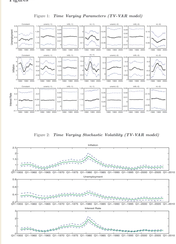
In order to understand if time variation is an important characteristic of the dataset, we estimate the TV-VAR model over the all sample and plot the estimated parameters and the standard deviation of the residuals (with the conﬁdence bands) over time.

Figure 1 in Appendix shows the evolution of the coeﬃcients over the sample. Many

13_{In the simulation exercise forecasts for horizon} _h_{= 1 correspond to nowcast, given that in real time} data are available only up to the previous quarter.

(16)

of them display constant patterns, while about four parameters are characterized by re-markable ﬂuctuations over time. Figure 2 shows evolution of the standard deviation of the residuals. All the volatilities exhibit accentuate time variation over the sample. The ﬁgure also shows that, concomitant with the great moderation period (middle 1980s), there is a sharp drop in the volatility of the residuals.

All in all these results show that time variation is an important features of the data. Modeling such feature in both coeﬃcients and variance is crucial for an accurate estimation and a correct interpretation of the results.

3.3 Other forecasting models

We compare the forecast obtained with the TV-VAR with those obtained using different standard forecasting models. First, we consider Time Varying Autoregressions (TV-AR) for each for the three series. We will keep the same specification and prior beliefs used for the TV-VAR. Second, we also consider univariate (AR) and multivariate (VAR) forecasts produced using fixed coefficient models. For sake of comparability, all the models are estimated with two lags. The models are estimated either recursively (REC), i.e. using all the data available at the time the forecast are made or using a rolling (ROL) window, i.e using the most recent ten years of data available at the time the forecast are made. The estimation over a rolling window is a very simple device to take time variation into account. The forecasts computed recursively and with rolling windows (on the VAR and AR models) will be denoted by VAR-REC, VAR-ROL, AR-REC, and AR-ROL respectively. Notice that the models predict quarterly inflation, therefore the forecasts for the h− quarter inflation

πh

t+h are computed by cumulating the ﬁrsth forecasts of the ﬁrst entries (which correspond

toπ_t) of the forecasted vector ˆy_t₊_h_|_t, that is ˆπh

t+h|t= h1

_h

i=1πˆt+i|t.

We will also compute no-change forecasts which are used as a benchmark. According to this na¨ıve model, unemployment and interest rate nexth−quarter ahead are predicted to be equal to the value observed in the current quarter. In the case of inflation we use a different benchmark. Atkeson and Ohanian (2001) showed that, since 1984, structural models of US inflation have been outperformed by a na¨ıve forecasts based on the average rate of inflation over the current and previous three quarters. This is essentially a ”no

(17)

change” forecast for annual inﬂation:

ˆ

π_th,ao₊_h_|_t=π4_t = 1

4(πt+πt−1+πt−2+πt−3) (7)

3.4 Forecast evaluation

Forecast accuracy is evaluated by means of the Mean Square Forecast Error (MSFE). The MSFE is a measure of the average forecast accuracy over the out-of-sample window. In the empirical exercise we use two samples to evaluate forecasting accuracy. The full sample, 1970 :Q1−2007 :Q4 and the sample 1985 :Q1−2007 :Q4. This latter period corresponds to the great moderation period. To facilitate the comparison between various models, the results are reported in terms of relative MSFE statistics, that is the ratio between the MSFE of a particular model to the MSFE of the na¨ıve model, used as the benchmark. When the relative MSFE is less than one, forecasts produced with a given non-benchmark model are, on average, more accurate that those produced with the benchmark model. For example, a value of 0.8 indicates that the model under consideration improves upon the benchmark by 20%.

4 Results

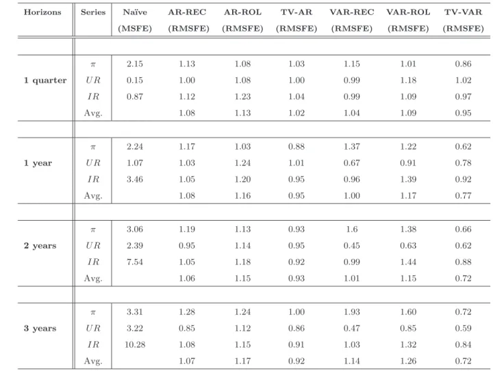
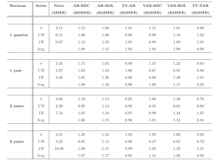
This section discusses the main ﬁndings of the forecasting exercise. Table 2 summarizes the results of the real time forecast evaluation, over the whole sample, for the three variables (inﬂation rate π_t, unemployment rate U R_t and the interest rateIR_t), and for the forecast horizons of one quarter, one year, two years and three years ahead. For the benchmark na¨ıve models we report the MSFE, while for the remaining models we report the MSFE relative to that of the na¨ıve model (RMSFE). The overall performance of each model is summarized, at each horizon, by averaging over the three variables.

Overall the TV-VAR produces very accurate forecasts for all the variables and, on average, performs better than any other model considered. In particular it outperforms the na¨ıve benchmark for all the variables at all horizons with gains ranging from 5 to 28 percent.

(18)

The best relative performances of the TV-VAR model is obtained for inﬂation. For this variable, the TV-VAR model produces the best forecast with an average (over the horizons) improvements of about 30% relative to the benchmark. A relative good performance is also observed for the TV-AR with improvements of about 10% at horizons of 1 and 2 years. The other time invariant speciﬁcations, univariate and multivariate, fail to improve upon the benchmark in terms of forecasting accuracy.

For interest rates, the varying parameter univariate and multivariate models perform similarly and they both improve upon constant parameter models. The advantage of the time-varying over constant parameter models is less clear cut for unemployment and interest rate. For unemployment, especially at long horizons, all models display good forecasting performances relative to the ”na¨ıve”benchmark. Notice, however, that the TV-VAR per-forms well for all horizons.

In conclusion, the TV-VAR model is the only one which does well systematically across variables and horizons.

These findings show that time varying models are quicker than fixed parameters spec-ifications to recognize structural changes in the permanent components of inflation and interest rate. They also suggest that interrelationships among macroeconomic variables carry out important information for forecasting, especially for unemployment and inflation, given that the accuracy of the multivariate time varying specification is always better than that of the univariate counterparts.

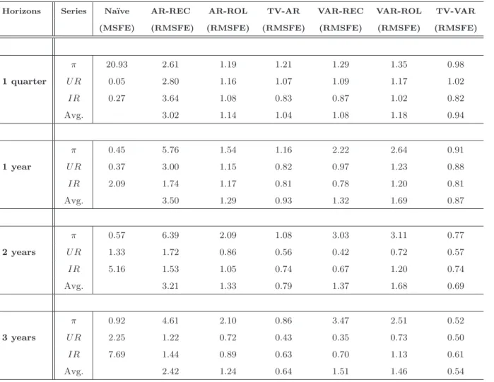
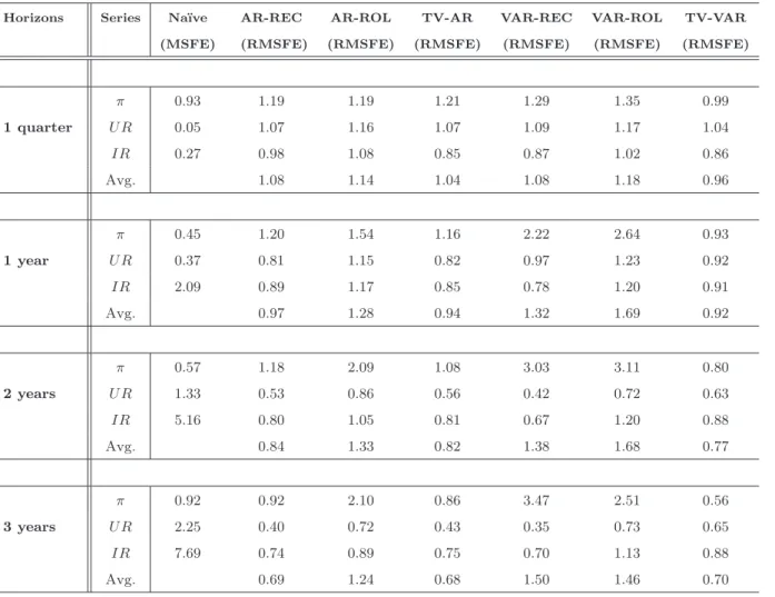
Table 3 shows the results for the “Great Moderation” period. Such a period is of par-ticular interest because it has been shown that it is extremely difficult to produce forecasts which are more accurate than those obtained with simple na¨ıve random walk models; how-ever, also in this period, most of the earlier findings are confirmed. First, the TV-VAR model generates the most accurate forecasts for all the variables. Second, the TV-VAR is again the model producing the best forecast for inflation with an average improvement (over the horizons) of about 30% on the random walk. In particular, the model performs very well for long run inflation forecasts, the improvement at the 3 years horizon is almost double that of the full sample, it is now about 52%; therefore the predictability of inflation can be reestablished once we account for structural changes. This is in line with Cogley,

(19)

Primiceri, and Sargent (2008) and Stock and Watson (2008b) who point out that the death of the Phillips curve is an artifact due to the neglected inﬂation trends and non-linearities. Third, forecasts of the interest rate obtained with the time varying models are more accu-rate than those in the previous sample. This might reﬂect the increased importance of the systematic predictable component of monetary policy in the last two decades. Finally, time varying methods also display more accurate forecasts, relative to the previous sample, for the unemployment rate series, over the longer horizons.

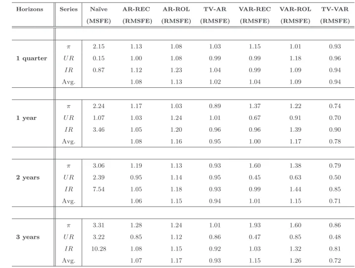
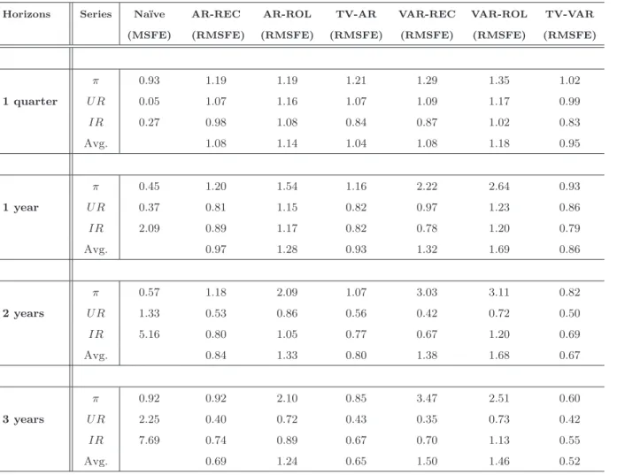
Finally, Tables 4-7 report the results of two different forecast simulations over the two samples. In the first one we use a more stringent priors specification to generate the fore-casts. By more stringent we mean that we assume ana priori smaller degree of variation in all the coefficients. Results are comparable, in terms of accuracy, with those obtained with the previous specification. The general message is that forecasts are particularly accurate when we attribute low probabilities of structural change. In the second simulation, we keep the explosive draws generated in the Gibb sampler algorithm. In this case the accuracy of the forecasts deteriorates for all the variables and in particular for the unemployment rate and interest rate. Similar result have been found by Clark and McCracken (2007) for longer term forecasts. This result, we believe, is especially interesting since there is no clear con-sensus about whether explosive draws should be discarded or not. Our results indicate that adjusting estimates to discard explosive roots is needed to improve out-of-sample forecast accuracy.

Figure 3 in Appendix shows the forecasts, obtained with and without the explosive roots, for the three variables at three years horizon. The main differences between the forecasts are on the first part of the sample until mid 1980s. Forecasts which include explosive draws are more volatile (this is true for inflation and interest rate). This is due to higher persistence of the series during those years, as consequence there is a higher probability to draw explosive roots and as consequence long-term forecasts tend to deviate from the unconditional mean. After the mid 1980s the forecasts generated with and without explosive roots display similar patterns.

(20)

5 Conclusions

The US economy has changed substantially during the post-WWII period. This paper tries to assess whether explicitly modeling these changes can improve the forecasting accuracy of key macroeconomic time series.

We produce real time out-of sample forecasts for inflation, the unemployment rate and a short term interest rate using time-varying coefficients VAR with stochastic volatility and we compare its forecasting performance to that of other standard models. Our findings show that the TV-VAR is the only model which systematically delivers accurate forecasts for the three variables. For inflation, the forecasts generated by the TV-VAR are much more accurate than those obtained with any other model. These results hold for the Great Moderation period (after mid 1980’s). This is particularly interesting since previous studies found that over this sample forecasting models have considerable difficulty in outperforming simple na¨ıve models in predicting many macroeconomic variables, in particular inflation.

We draw two main conclusions. First, taking into account structural economic change is important for forecasting. Second, the TV-VAR model is a very powerful tool for real-time forecasting since it incorporate in a ﬂexible but parsimonious manner the prominent features of a time-varying economy.

This is a ﬁrst step in the investigation of how structural change can be explicitly modeled for improving macroeconomic forecasting. We have assessed the accuracy of point forecasts. The assessment of real-time accuracy of density forecasts is an interesting road for future research since, as pointed out by Cogley, Morozov, and Sargent (2005), the TV-VAR model is well suited to characterizing also forecasting uncertainty, in particular for inﬂation in a situation in which monetary policy and the economy are subject to ongoing changes.

(21)

References

Atkeson, A., and L. E. Ohanian (2001): “Are Phillips Curves Useful for Forecasting

Inﬂation?,” Quarterly Review, pp. 2–11.

Canova, F. (2007): “G-7 Inﬂation Forecasts: Random Walk, Phillips Curve Or What

Else?,” Macroeconomic Dynamics, 11(01), 1–30.

Carter, C. K., and R.Kohn (1994): “On Gibbs Sampling for State Space Models,”

Biometrika, 81, 541–553.

Clarida, R., J. Gali, andM. Gertler(2000): “Monetary Policy Rules And

Macroeco-nomic Stability: Evidence And Some Theory,” Quarterly Journal of Economics, 115(1), 147–180.

Clark, T. E., and M. W. McCracken(2007): “Forecasting with small macroeconomic

VARs in the presence of instabilities,” Discussion paper.

Cogley, T., S. Morozov,and T. J. Sargent(2005): “Bayesian fan charts for U.K.

in-ﬂation: Forecasting and sources of uncertainty in an evolving monetary system,” Journal of Economic Dynamics and Control, 29(11), 1893–1925.

Cogley, T., G. E. Primiceri, and T. J. Sargent (2008): “Inﬂation-Gap Persistence

in the U.S.,” NBER Working Paper 13749, NBER.

Cogley, T.,andT. J. Sargent(2001): “Evolving Post WWII U.S. Inﬂation Dynamics,”

inMacroeconomics Annual, pp. 331–373. MIT Press.

(2005): “Drifts and Volatilities: Monetary Policies and Outcomes in the Post WWII US,” Review of Economic Dynamics, 8, 262–302.

D’Agostino, A., D. Giannone,andP. Surico(2006): “(Un)Predictability and

Macroe-conomic Stability,” Working Paper Series 605, European Central Bank.

Doan, T., R. Litterman, andC. A. Sims(1984): “Forecasting and Conditional

(22)

Giannone, D., M. Lenza, andL. Reichlin(2008): “Explaining The Great Moderation:

It Is Not The Shocks,” Journal of the European Economic Association, 6(2-3), 621 – 633.

Pivetta, F., and R. Reis (2007): “The Persistence of Inﬂation in the United States,”

Journal of Economic Dynamics and Control, 31, No.4, 1326–1358.

Primiceri, G. E.(2005): “Time Varying Structural Vector Autoregressions and Monetary

Policy,” Review of Economic Studies, 72, 821–852.

Roberts, J. M. (2006): “Monetary Policy and Inﬂation Dynamics,”ijcb, 2(3), 193–230. Romer, David, H.,and C. Romer(2000): “Federal Reserve Information and the

Behav-ior of Interest Rates,” American Economic Review, 90, 429 – 457.

Rossi, B.,andT. Sekhposyan_{(2008): “as models forecasting performance for US output}

growth and inﬂation changed over time, and when?,” Manuscript, Duke University.

Sbordone, A. M., and T. Cogley(2008): “Trend Inﬂation and Inﬂation Persistence in

the New Keynesian Phillips Curve,”American Economic Review, forthcoming.

Staiger, D., J. H. Stock, and M. W. Watson (2001): “Prices, Wages, and the U.S.

NAIRU in the 1990s,” in In The Roaring Nineties: Can Full Employment Be Sustained?, ed. by A. B. Krueger, andR. M. Solow. Russell Sage Foundation.

Stock, J. H.,andM. W. Watson(1996): “Evidence on Structural Instability in

Macroe-conomic Time Series Relations,”Journal of Business & Economic Statistics, 14(1), 11–30.

Stock, J. H.,andM. W. Watson(2004): “Has the Business Cycle Changed and Why?,”

inNBER Macroeconomics Annual 2003, ed. by M. Gertler,andK. Rogoﬀ. MIT Press.

(2007): “Why Has U.S. Inﬂation Become Harder to Forecast?,”Journal of Money, Credit and Banking, 39, No.1.

(2008a): “Phillips Curve Inﬂation Forecasts,” NBER Working Paper 14322, NBER.

(2008b): “Phillips Curve Inﬂation Forecasts,” NBER Working Paper 2005-42, 14322.

(23)

Appendix

Estimation is done using Bayesian methods. To draw from the joint posterior distribution of model parameters we use a Gibbs sampling algorithm along the lines described in Primiceri (2005). The basic idea of the algorithm is to draw sets of coeﬃcients from known condi-tional posterior distributions. The algorithm is initialized at some values and, under some regularity conditions, the draws converge to a draw from the joint posterior after a burn in period. Letz be (q×1) vector, we denote zT _{the sequence [}_z

1, ..., zT]. Each repetition is

composed of the following steps:

1. p(σT_|_xT_{, θ}T_{, φ}T_,_Ω_,_Ξ_,_Ψ_{, s}T₎ 2. p(sT_|_xT_{, θ}T_{, σ}T_{, φ}T_,_Ω_,_Ξ_,_Ψ)14 3. p(φT_|_xT_{, θ}T_{, σ}T_,_Ω_,_Ξ_,_Ψ_{, s}T₎ 4. p(θT_|_xT_{, σ}T_{, φ}T_,_Ω_,_Ξ_,_Ψ_{, s}T₎ 5. p(Ω|xT, θT, σT, φT,Ξ,Ψ, sT) 6. p(Ξ|xT, θT, σT, φT,Ω,Ψ, sT) 7. p(Ψ|xT, θT, σT, φT,Ω,Ξ, sT)

Gibbs sampling algorithm

• Step 1: sample fromp(σT_|_yT_{, θ}T_{, φ}T_,_Ω_,_Ξ_,_Ψ_{, s}T₎

To drawσT we use the algorithm of Kim, Shephard and Chibb (KSC) (1998). Consider the system of equationsy∗_t ≡F_t−1(y_t−X_tθ_t) =D_t1/2u_t, whereu_t∼N(0, I),X_t= (I_n⊗x_t), and x_t = [1_n, y_t₋₁...y_t₋_p]. Conditional on yT, θT, and φT, y_t∗ is observable. Squaring and taking the logarithm, we obtain

y∗∗_t = 2r_t+υ_t (8)

r_t=r_t₋₁+ξ_t (9)

(24)

wherey_i,t∗∗= log((y_i,t∗ )2+ 0.001) - the constant (0.001) is added to make estimation more ro-bust -υ_i,t = log(u2_i,t) andr_t= logσ_i,t. Since, the innovation in (8) is distributed as logχ2(1), we use, following KSC, a mixture of 7 normal densities with component probabilities q_j, means m_j −1.2704, and variances v2_j (j=1,...,7) to transform the system in a Gaussian one, where{q_j, m_j, v_j2}are chosen to match the moments of the logχ2(1) distribution. The values are:

Table 1: Parameters Speciﬁcation

j q_j m_j v2_j 1.0000 0.0073 -10.1300 5.7960 2.0000 0.1056 -3.9728 2.6137 3.0000 0.0000 -8.5669 5.1795 4.0000 0.0440 2.7779 0.1674 5.0000 0.3400 0.6194 0.6401 6.0000 0.2457 1.7952 0.3402 7.0000 0.2575 -1.0882 1.2626

Let sT = [s₁, ..., s_T] be a matrix of indicators selecting the member of the mixture to

be used for each element of υ_t at each point in time. Conditional on sT_{, (}_υ_i,t|_s

i,t = j) ∼

N(m_j −1.2704, v_j2). Therefore we can use the algorithm of Carter and R.Kohn (1994) to draw r_t (t=1,...,T) from N(r_t_|_t₊₁, R_t_|_t₊₁), where r_t_|_t₊₁ = E(rt|r_t₊₁, yt_{, θ}T_{, φ}T_,_Ω_,_Ξ_,_Ψ_{, s}T_,₎

andR_t_|_t₊₁=V ar(rt|r_t₊₁, yt, θT, φT,Ω,Ξ,Ψ, sT).

• Step 2: sample fromp(sT_|_yT_{, θ}T_{, σ}T_{, φ}T_,_Ω_,_Ξ_,_Ψ)

Conditional on y∗∗_i,t and rT_{, we independently sample each} _s

i,t from the discrete density

deﬁned byP r(s_i,t=j|y∗∗_i,t, r_i,t)∝f_N(y_i,t∗∗|2r_i,t+m_j−1.2704, v_j2), wheref_N(y|μ, σ2) denotes a normal density with meanμand varianceσ2.

• Step 3: sample fromp(φT|yT, θT, σT,Ω,Ξ,Ψ, sT)

Consider again the system of equationsF_t−1(y_t−X_tθ_t) =F_t−1yˆ_t=D_t1/2u_t. Conditional onθT, ˆy is observable. SinceF−1 is lower triangular with ones in the main diagonal, each

(25)

equation in the above system can be written as

ˆ

y₁_,t = σ₁_,tu₁_,t (10)

ˆ

y_i,t = −yˆ_[1_,i₋_1]_,tφ_i,t+σ_i,tu_i,t i= 2, ..., n (11)

whereσ_i,t andu_i,t are theith elements of σ_t and u_t respectively, ˆy_[1_,i₋_1]_,t = [ˆy₁_,t, ...,yˆ_i₋₁_,t]. Under the block diagonality of Ψ, the algorithm of Carter and R.Kohn (1994) can be applied equation by equation, obtaining draws for φ_i,t from a N(φ_i,t_|_t₊₁,Φ_i,t_|_t₊₁), where

φ_i,t_|_t₊₁ =E(φi,t|φ_i,t₊₁, yt_{, θ}T_{, σ}T_,_Ω_,_Ξ_,_{Ψ) and Φ}

i,t|t+1 =V ar(φi,t|φi,t+1, yt, θT, σT,Ω,Ξ,Ψ). • Step 4: sample from p(θT_|_yT_{, σ}T_{, φ}T_,_Ω_,_Ξ_,_Ψ_{, s}T₎

Conditional on all other parameters and the observables we have

y_t=X_tθ_t+ε_t (12)

θ_t=θ_t₋₁+ω_t (13)

Draws forθ_tcan be obtained from aN(θ_t_|_t₊₁, P_t_|_t₊₁), whereθ_t_|_t₊₁ =E(θt|θ_t₊₁, yT, σT, φT,Ω,Ξ,Ψ) andP_t_|_t₊₁=V ar(θt|θ_t₊₁, yT_{, σ}T_{, φ}T_,_Ω_,_Ξ_,_{Ψ) are obtained with the algorithm of Carter and}

R.Kohn (1994).

• Step 5: sample from p(Ω|yT_{, θ}T_{, σ}T_{, φ}T_,_Ξ_,_Ψ_{, s}T₎

Conditional on the other coeﬃcients and the data, Ω has an Inverse-Wishart posterior density with scale matrix Ω−₁1 = (Ω₀ +T_t₌₁Δθ_t(Δθ_t))−1 and degrees of freedom df_Ω₁ =

df_Ω₀+T, where Ω−₀1 is the prior scale matrix,df_Ω₀ are the prior degrees of freedom andT is length of the sample use for estimation. To draw a realization for Ω makedf_Ω₁ independent drawsz_i(i=1,...,df_Ω₁) fromN(0,Ω₁−1) and compute Ω = (df_i₌₁Ω1z_iz_i)−1 (see Gelman et. al., 1995).

• Step 6: sample from p(Ξi,i|yT_{, θ}T_{, σ}T_{, φ}T_,_Ω_,_Ψ_{, s}T₎

Conditional the other coeﬃcients and the data, Ξ has an Inverse-Wishart posterior density with scale matrix Ξ−₁1 = (Ξ₀ +T_t₌₁Δ logσ_t(Δ logσ_t))−1 and degrees of freedom

df_Ξ₁ =df_Ξ₀ +T where Ξ−₀1 is the prior scale matrix anddf_Ξ₀ the prior degrees of freedom. Draws are obtained as in step 5.

(26)

Conditional on the other coeﬃcients and the data, Ψ_i has an Inverse-Wishart posterior density with scale matrix Ψ−_i,₁1 = (Ψ_i,₀ +T_t₌₁Δφ_i,t(Δφ_i,t))−1 and degrees of freedom

df_Ψ_i,₁ = df_Ψ_i,₀ +T where Ψ−_i,₀1 is the prior scale matrix and df_Ψ_i,₀ the prior degrees of freedom. Draws are obtained as in step 5 for alli.

In the first estimation (the first out-of-sample forecast iteration), we make 12000 repeti-tions discarding the first 10000 and collecting one out of five draws. In the other estimarepeti-tions, we initialize the coefficients with the medians obtained in the previous estimation, and we make 2500 repetitions discarding the first 500 and collecting one out of five draws.

(27)

Table 2: Forecasting Accuracy over the sample: 1970-2007

Horizons Series Na¨ıve AR-REC AR-ROL TV-AR VAR-REC VAR-ROL TV-VAR (MSFE) (RMSFE) (RMSFE) (RMSFE) (RMSFE) (RMSFE) (RMSFE)

π 2.15 1.13 1.08 1.03 1.15 1.01 0.86 1 quarter UR 0.15 1.00 1.08 1.00 0.99 1.18 1.02 IR 0.87 1.12 1.23 1.04 0.99 1.09 0.97 Avg. 1.08 1.13 1.02 1.04 1.09 0.95 π 2.24 1.17 1.03 0.88 1.37 1.22 0.62 1 year UR 1.07 1.03 1.24 1.01 0.67 0.91 0.78 IR 3.46 1.05 1.20 0.95 0.96 1.39 0.92 Avg. 1.08 1.16 0.95 1.00 1.17 0.77 π 3.06 1.19 1.13 0.93 1.6 1.38 0.66 2 years UR 2.39 0.95 1.14 0.95 0.45 0.63 0.62 IR 7.54 1.05 1.18 0.92 0.99 1.44 0.88 Avg. 1.06 1.15 0.93 1.01 1.15 0.72 π 3.31 1.28 1.24 1.00 1.93 1.60 0.72 3 years UR 3.22 0.85 1.12 0.86 0.47 0.85 0.59 IR 10.28 1.08 1.15 0.91 1.03 1.32 0.84 Avg. 1.07 1.17 0.92 1.14 1.26 0.72

First column, horizons; second column, series; third column MSFE of na¨ıve models; other columns, relative MSFE, that is, ratio of the MSFE of a particular model to the MSFE of the na¨ıve model. For each horizon is also reported the average of the relative MSFE across variables (Avg.).

(28)

Table 3: Forecasting Accuracy over the sample: 1985-2007

(29)

Table 4: Forecasting Accuracy over the sample: 1970-2007 (More Stringent Priors)

First column, horizons; second column, series; third column MSFE of na¨ıve models; other columns, relative MSFE, that is, ratio of the MSFE of a particular model to the MSFE of the na¨ıve model. For each horizon is also reported the average of the relative MSFE across variables (Avg.). In this estimation we setλ1= 0.00001, λ2= 0.001andλ3= 0.00001.

(30)

Table 5: Forecasting Accuracy over the sample: 1985-2007 (More Stringent Priors)

First column, horizons; second column, series; third column MSFE of na¨ıve models; other columns, relative MSFE, that is, ratio of the MSFE of a particular model to the MSFE of the na¨ıve model. For each horizon is also reported the average of the relative MSFE across variables (Avg.). In this estimation we setλ₁= 0.00001,λ₂= 0.001and λ₃= 0.00001.

(31)

Table 6: Forecasting Accuracy over the sample: 1970-2007 (with Explosive Draws)

(32)

Table 7: Forecasting Accuracy over the sample: 1985-2007 (with Explosive Draws)

(33)

Figure 1: Time Varying Parameters (TV-VAR model) 1960 1983 2005 0 0.2 0.4 0.6 0.8 Unemployment Constant 1960 1983 2005 1.1 1.15 1.2 1.25 1.3 unem(−1) 1960 1983 2005 −0.01 0 0.01 0.02 0.03 0.04 0.05 infl(−1) 1960 1983 2005 −0.15 −0.1 −0.05 0 0.05 ir(−1) 1960 1983 2005 −0.4 −0.35 −0.3 −0.25 −0.2 unem(−2) 1960 1983 2005 −0.02 −0.01 0 0.01 0.02 0.03 0.04 infl(−2) 1960 1983 2005 0 0.05 0.1 0.15 0.2 ir(−2) 1960 1983 2005 0 1 2 3 4 5 Inflation Constant 1960 1983 2005 −1 −0.8 −0.6 −0.4 −0.2 0 unem(−1) 1960 1983 2005 0.2 0.25 0.3 0.35 0.4 0.45 infl(−1) 1960 1983 2005 −0.4 −0.2 0 0.2 0.4 0.6 ir(−1) 1960 1983 2005 −0.2 0 0.2 0.4 0.6 unem(−2) 1960 1983 2005 0 0.05 0.1 0.15 0.2 0.25 infl(−2) 1960 1983 2005 −0.6 −0.4 −0.2 0 0.2 0.4 ir(−2) 1960 1983 2005 −0.1 0 0.1 0.2 0.3 Interest Rate Constant 1960 1983 2005 −0.35 −0.3 −0.25 −0.2 −0.15 unem(−1) 1960 1983 2005 −0.01 0 0.01 0.02 0.03 0.04 infl(−1) 1960 1983 2005 1.05 1.1 1.15 1.2 1.25 ir(−1) 1960 1983 2005 0.2 0.25 0.3 0.35 0.4 unem(−2) 1960 1983 2005 −0.02 −0.01 0 0.01 0.02 0.03 infl(−2) 1960 1983 2005 −0.3 −0.25 −0.2 −0.15 −0.1 ir(−2)

Figure 2: Time Varying Stochastic Volatility (TV-VAR model)

Q10.5−1955 Q1−1960 Q1−1965 Q1−1970 Q1−1975 Q1−1980 Q1−1985 Q1−1990 Q1−1995 Q1−2000 Q1−2005 Q1−2010 1 1.5 2 2.5 Inflation Q10.2−1955 Q1−1960 Q1−1965 Q1−1970 Q1−1975 Q1−1980 Q1−1985 Q1−1990 Q1−1995 Q1−2000 Q1−2005 Q1−2010 0.4 0.6 0.8 Unemployment 2 3 Interest Rate

FiguresSS

(34)

Figure 3: Three Years Ahead Forecast Q10−1970 Q1−1975 Q1−1980 Q1−1985 Q1−1990 Q1−1995 Q1−2000 Q1−2005 Q1−2010 5 10 15 Q10−1970 Q1−1975 Q1−1980 Q1−1985 Q1−1990 Q1−1995 Q1−2000 Q1−2005 Q1−2010 5 10 15 Unemployment Q10−1970 Q1−1975 Q1−1980 Q1−1985 Q1−1990 Q1−1995 Q1−2000 Q1−2005 Q1−2010 5 10 15 20 Interest Rate True Values Explosive Roots Stable Roots