Received December 25, 2019, accepted February 6, 2020, date of publication March 6, 2020, date of current version March 27, 2020. Digital Object Identifier 10.1109/ACCESS.2020.2979012
A Dynamic Bayesian Network Approach for
Analysing Topic-Sentiment Evolution
HUIZHI LIANG , UMARANI GANESHBABU, AND THOMAS THORNE Department of Computer Science, University of Reading, Reading RG6 1DP, U.K.
Corresponding authors: Huizhi Liang ([email protected]) and Thomas Thorne ([email protected])
ABSTRACT Sentiment analysis is one of the key tasks of natural language understanding. Sentiment Evolution models the dynamics of sentiment orientation over time. It can help people have a more profound and deep understanding of opinion and sentiment implied in user generated content. Existing work mainly focuses on sentiment classification, while the analysis of how the sentiment orientation of a topic has been influenced by other topics or the dynamic interaction of topics from the aspect of sentiment has been ignored. In this paper, we propose to construct a Gaussian Process Dynamic Bayesian Network to model the dynamics and interactions of the sentiment of topics on social media such as Twitter. We use Dynamic Bayesian Networks to model time series of the sentiment of related topics and learn relationships between them. The network model itself applies Gaussian Process Regression to model the sentiment at a given time point based on related topics at previous time. We conducted experiments on a real world dataset that was crawled from Twitter with 9.72 million tweets. The experiment demonstrates a case study of analysing the sentiment dynamics of topics related to the event Brexit.
INDEX TERMS Sentiment analysis, sentiment evolution, dynamic Bayesian network, social media, temporal dynamics.
I. INTRODUCTION
Opinions are central to almost all human activities. Sentiment analysis is the field of study that analyses people’s opin-ions and sentiments. The rise of opinion-rich user behaviour resources such as online review sites, blogs and micro-blogs (e.g., Twitter) has fuelled interest in sentiment analysis [1], [2]. Sentiment analysis has been shown to have utility in various business intelligence applications, including product marketing, identifying new business opportunities, and man-aging a company’s reputation [1], [2].
Every day massive numbers of instant messages are pub-lished on social media platforms such as Twitter and Weibo. On these platforms, users express their real feelings and opinions freely. Hashtags, starting with a symbol ahead of keywords or phrases, are widely used in tweets as coarse-grained topics [3], [4] and hashtags have been widely used on Twitter (27% of tweets contain hashtags [4], [5]). For example, the hashtag ‘‘#Brexit’’ has recently been a trending topic on Twitter for a long period of time. Sentence or tweet level sentiment analysis results can provide very useful
The associate editor coordinating the review of this manuscript and approving it for publication was Yong Xiang .
information [4], and most existing sentiment analysis work focuses on this task [6]. For example, using natural language processing approaches such as Convolutional Neural Net-works [7] to predict whether the sentiment polarity of a given tweet is ‘‘Positive’’ , ‘‘Negative’’ , or ‘‘Neutral’’.
On the other hand, topic level or hashtag level sentiment analysis that detects the overall or general sentiment tendency towards topics is also important in many scenarios [4], [6]. For example, people’s overall sentiment tendency on the topic ‘‘#Brexit’’ on Twitter will be an important indicator of the outcome of political events. Another example is that the topic level sentiment origination of a new product ‘‘#iphone10’’ can be used for the prediction of sales of this new phone model [4], and even the stock price of the relevant com-pany [8]. However, people are not only interested in the sentiment tendency of one topic, but also want to know how the sentiment of a topic has been been influenced by other topics over time. For example, how the sentiment of the topic ‘‘#Brexit’’ has been influenced by other related topics. In all these scenarios, comprehensive topic level sentiment dynamics analysis is needed.
Sentiment Evolution models the dynamics of sentiment orientation over time. It can help people have a more profound
and deep understanding of opinion and sentiment implied in user generated content [9]. Existing work focuses on latent topic sentiment dynamics detection on long text documents such as reviews [10] or blogs [11], while hashtag based topic sentiment dynamics analysis usually focuses on sentiment time series visualization [12] or spike explaination [13]. For example, some systems such as [3], [14] have been proposed to visualise the sentiment of topics over time. Some work [12] has been proposed to analyse sentiment time series data such as frequency analysis [12], outlier detection [12], or explain-ing the trigger of a spike [13]. How the sentiment orientation of a topic has been influenced by other topics and the anal-ysis or modelling of the dynamic interactions of topics from the aspect of sentiment have been ignored by existing work.
Dynamic Bayesian Networks (DBNs) have been popularly used for modelling the dynamic interaction of multiple enti-ties in time series data such as gene regulatory networks [15]–[18], speech analysis [19] and other application areas [20], [21]. How to apply them for analysing sentiment evolution still remains an open research question. In this paper, we propose to apply DBNs to the sentiment evolution domain and use them to model the dynamics and interactions of the sentiment of topics on social media.
The major contributions of this paper are as follows: • This is the first work to use a Dynamic Bayesian
Network to model the dynamics and interactions of the sentiment of topics. It can provide more in-depth sentiment analysis for social media.
• This work proposes to construct a Gaussian Process Dynamic Bayesian Network to model time series of the sentiment of related topics and learn relation-ships between them.
• This work develops a Sequential Monte Carlo sam-pler to perform Bayesian inference on a Dynamic Bayesian Network model.
• This work conducted experiments on a real dataset that was crawled from twitter with 9.72 million tweets and shows results of a case study of analysing the sentiment dynamics of hashtags related to the event Brexit.
The rest of the paper is organised as follows. In Section 2, related work will be briefly reviewed. Then the proposed approaches will be discussed in detail in Section 3, with a detailed discussion of how to learn a DBN for sentiment evolution. In Section 4, the experiments and results will be discussed. The conclusions will be given in Section 5.
II. RELATED WORK
Sentiment analysis has attracted more and more attention from researchers in recent years. Due to the complexity of human natural language, the problem of sentiment analysis remains an open question. One of the popular tasks of senti-ment analysis is to classify a sentence or docusenti-ment into dif-ferent categories or classes using the 5 or 10-point scale, or a simple three-label class set of ‘‘Positive’’ , ‘‘Negative’’ and ‘‘Neutral’’ [1], [2]. For sentence and document level
sentiment classification tasks, traditionally a rich set of hand-tuned features such as word-sentiment association lex-icon features, word n-grams, punctuation, and emoticons extracted from the content were selected as representative text features [22]–[25]. Based on the text features, a sim-ple SVM-based classifier [26] was used to to conduct sen-timent classification. Deep learning techniques [27] have recently emerged as a promising framework for sentiment classification tasks. Approaches such as convolutional neural networks [7], recurrent neural networks [28], and attention models [29] can achieve the state-of-the-art performance for both sentence and document level sentiment classification.
Sentiment analysis can also be dependent upon a partic-ular topic [4], [9], [30], entity or event [31]. Topics can be classified as explicit topics such as keywords or hashtags [4] given or implicit topics such as latent or hidden topics gener-ated by dimension reduction algorithms [30]. The majority of implicit topic-dependent sentiment analysis approaches jointly model the topics and sentiment with extended LDA models [11], [30]. For example, Rahman and Wang [30] proposed a hidden topic sentiment model to explicitly capture topic coherence and sentiment consistency for the purpose of predicting the sentiment polarities. The implicit topic based approaches are more applicable for long documents that con-tain multiple topics. In the research of short text such as micro-blogs, hashtags have been popularly used as explicit topics [3], [14]. For example, Zhao et al.[3] presented a Social Sentiment Sensor (SSS) system on Sina Weibo to detect daily hot topics based on hashtags and analyse the sentiment distributions toward these topics. For a given topic, the most popularly used approach is to aggregate the sen-timent of each sentence or document that belongs to this topic [32]. Other approaches from the macro level perspective to detect the sentiment of a topic have been proposed. For example, Wanget al. [4] proposed a graph based approach to detect the sentiment of topics based on the co-occurrence information of hashtags. Most existing approaches focus on static topic-sentiment conjugations or predictions, failing to capture the dynamics of sentiment on topics.
Sentiment evolution is another sentiment analysis task that has attracted increasing attention from both academia and industry recently [6]. It is able to capture the senti-ment dynamics of topics over time, and thus can provide a more in-depth analysis of textural data [6]. Some approaches such as dynamic joint sentiment-topic model [33], neighbour-hood based influence propagation model, and location-based dynamic sentiment-topic models [34] have been proposed to capture the evolution of the sentiment of topics. Sentiment time series have been used to track sentiments of public topics and make predictions [8], for example, work in the literature proposed a location sentiment evolution model to track the sentiment of topics in natural disasters [34], while Siet al.[8] proposed a continuous Dirichlet process mixture model to learn the daily topic set and build sentiment time series for each topic, and then used it to predict the stock market. Some systems such as [3], [14] have been proposed to visualise the
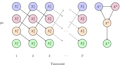
FIGURE 1. Dynamic Bayesian Network model of sentiment evolution. Sentiment on a topiciat timet, measured asXtiis dependent on the sentiment at the previous timepoint,Xt−1. This allows the
network structure shown on the right, which includes a directed cycle, to be represented as a graphical model, using the DBN structure shown on the left.
TABLE 1. Notation used for methods.
sentiment of topics over time. However, how the sentiment orientation of a topic has been influenced by other topics and the dynamic interaction of topics from the aspect of sentiment have been ignored by existing work.
Bayesian networks [35] can model the conditional inde-pendence relationships between variables, learning directed acyclic graphs that represent a factorisation of the joint prob-ability distribution over the relevant variables. These models do not take into account temporal information, and the restric-tion to acyclic graph structures means they cannot model various phenomena that occur in time series data. These static Bayesian network models have been proposed to model the sentiment of topics previously in the literature [10], [36]. However, Bayesian networks cannot include temporal infor-mation in the model, while Dynamic Bayesian Networks [37] are able to model the temporal relationships between data points in a time series. In this paper, we propose to apply DBNs to the sentiment evolution domain and use it to model the dynamics and interactions of the sentiment of topics in social media.
III. LEARNING DYNAMIC BAYESIAN NETWORKS FOR SENTIMENT EVOLUTION
We apply Markov Chain Monte Carlo (MCMC) method to learn the network structure, as it allows us to estimate the
posterior distribution over network structures in a Bayesian framework, giving an estimate of the posterior probability of each possible edge. For the DBN conditional distributions we apply Gaussian Process regression, as this approach is flexible and can model non-linear dependencies. In this paper, a topic is defined as a hashtag. The two terms topic and hashtag are used interchangeably.
We use a DBN to model the evolution of sentiment over time and learn the relationships between topics. The DBN models a topiciat a timepointtas having a distribution that is conditional on the values of a set of parent topics, Pa(i) at the previous timepoints, in our case only depending on the previous timepointt−1. This is illustrated in figure1. Then for topicsi = 1, . . . ,P, at timest = 1, . . . ,T, we denote the sentiment on topici at timet as Xti, and in the DBN model
p(Xti|Xt−1, θ)=f(XtPa(−1i), θ) (1)
whereXt−1denotes the sentiment of all the topics at timet−1,
f is a function of the parents of variableiat timet−1, and a set of parametersθ. We exclude the variableifrom being a member of its own parent set Pa(i).
The main focus of this paper is to learn whether the senti-ment of topics depend on one another, rather than learning the exact nature of the dependence between the sentiment on top-ics. This can be thought of as learning which topics influence the sentiment of others, by inferring conditional dependencies between topics. In this work we take the approach of using a flexible nonparametric regression model, Gaussian Process Regression [38], that allows the marginal likelihood to be evaluated directly. Gaussian Processes are a nonparametric model that allows us to place a prior on the function f in equation 1, and which have been used successfully in pre-vious work in the literature to learn DBNs from time series data [39], [40].
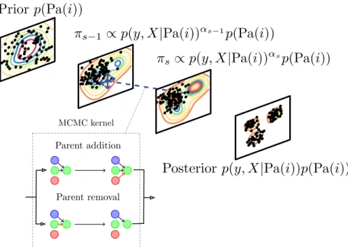
FIGURE 2. Sequential Monte Carlo sampler for Dynamic Bayesian Networks. Particles (parent sets for topici) are sampled for the prior, then through several intermediate stages particles are perturbed with an MCMC kernel, to reach the posterior target.
A. GAUSSIAN PROCESS REGRESSION
To model the dependency of a variable on its parent set, we apply Gaussian process regression [38]. This treats the observationsyas following a multivariate normal distribution with some covariance6 that is defined by a kernel on the predictorsD. For observations of the sentiment of a single topic at T timepoints,y1, . . . ,yT andPtopics on which it may depend in aT ×PmatrixD, we define
y∼N(0, 6y,D) (2) where the covariance matrix6y,Dis defined using a kernelK on the predictors
6i,j=K(Di,Dj)+I(i=j)σy2, (3) with the termσy2accounting for noise in the observations,Di denoting rowiinDandIdenoting the indicator function.
For the kernel K we have chosen the commonly used squared exponential kernel, which has two parameters, the length scalel, and the heightσf2
K(Di,Dj)=σf2exp
(Di−Dj)2
2l2 . (4)
To apply this in our DBN model, the sentiment of a topic i for which we wish to learn the parent set Pa(i) becomes y=X2i:T and the remaining topicsD=X1:(T−1), introducing
a time lag of one interval betweenyandD.
As our main aim is to learn the membership of the parent set of each variable, we can marginalise out the parameters of the likelihood and obtain a marginal likelihood that only
depends on the selection of parents, as p(y|D)=
Z
p(y|f,D)p(f|D)df =N(y|0, 6y,D) (5) which can be used to construct the posterior distribution on parent sets Pa(i) for a topicias
p(Pa(i)|D)∝p(y|DPa(i))p(Pa(i)) (6) wherep(Pa(i)) is the prior on the parent sets, andDPa(i)is the sentiment of the parent topics. Here we set the prior for all topics as a Poisson distribution on the size of the parent set with rate parameterλ =2, including edges uniformly. This remains constant throughout the inference procedure. B. MARKOV CHAIN MONTE CARLO
Applying Gaussian process regression and our prior on the parent sets, we can construct a Bayesian model of sentiment evolution over time with posterior distribution as defined in equation6.
We would then like to estimate the posterior distribution over parent sets Pa(i) for each topic i = 1, . . . ,P, and in this case we can do so by sampling from the posterior using Markov Chain Monte Carlo methods [41]. As we can calculate the marginal likelihood, it would also be possi-ble to directly evaluate the posterior for each possipossi-ble par-ent set. However if we allow for large numbers of topics, and potentially many parent topics influencing sentiment per topic, the number of possible combinations of parents for each variable quickly becomes too large to evaluate the posterior of each. In previous work in the literature, this has been addressed by limiting the size of potential parent
Algorithm 1Sequential Monte Carlo Sampler
1: Input:Sentiment time series for topiciand all potential parents.
2: Output:Set ofM parent sets for topici.
3: Sample particles Pa1(i), . . . ,PaM(i) fromp(Pa(i))
4: Set particle weightsw1,1, . . . ,wM,1=M1 5: s←1
6: αs ←0
7: whileαs<1do
8: Increments
9: findαssuch thatESSis greater than threshold
10: form∈ 1, . . . ,M do 11: wm,s ←wm,s−1γγs(Pam(i)) s−1(Pam(i)) 12: end for 13: Normalisewm,s 14: Resample particles 15: form∈ 1, . . . ,M do
16: Sample Pam(i) from MCMC kernel
17: end for
18: end while
sets [39], [40] to reduce the possible numbers of parent sets that must be evaluated. In contrast, here we extend this approach by applying a Sequential Monte Carlo sampler [42] that considers multiple possible parent sets at once, in paral-lel, and can draw samples from the posterior distribution over network structures for parent sets of unlimited size.
Using an SMC sampler to sample from the posterior defined above, the parameter space is explored by multi-ple particles (values of the model parameters) over a num-ber of discrete steps, slowly moving from a sample of particles from the prior distribution, to the full posterior, as illustrated in figure 2. In contrast with the majority of MCMC methods, the SMC sampler is less prone to becoming stuck in local maxima of the target distribution, as it does not rely on a single state. The SMC algorithm is outlined in algorithm1.
The sampler proceeds by generating a weighted population of M parameter estimates for the model, known as parti-cles, targeting a particular distribution over several iterations. As we are aiming to estimate a posterior distribution on parent sets for a given topic, we apply Sequential Monte Carlo by moving from the prior distribution to include the likelihood over multiple steps before arriving at the posterior. The initial set of particles are sampled directly from the prior on parent sets, and propagated between steps using a kernel to perturb the particles and reduce degeneracy.
In each step of the Sequential Monte Carlo algorithm we define the (unnormalised) target distribution over parent sets at steps∈ 1. . .Sas
γs(Pa(i))=p(y|DPa(i))αsp(Pa(i)) (7) where 0 ≤ αs ≤ 1, for some increasing sequence of αs, with α1 = 0 and αS = 1. For α1 = 0 theM particles
can be sampled directly from the prior, and are given equal
weights wm,1 = M1 for m = 1, . . . ,M. Moving between
the targetγs−1 andγs, the particles, written as Pam(i), are assigned weightswm,s so that the normalised posteriorπsis approximated by πs(Pa(i))= M X m=1 wm,sδPam(i), (8)
whereδ is the Dirac delta function. The particles are then perturbed using a kernel. In models with continuous param-eter spaces it is possible to use a simple Gaussian kernel to move particles in the parameter space. In our case as the parameters associated with each particle are discrete, we must define a suitable kernel on the parameter space, and so we define a Markov Chain Monte Carlo kernel, with the target at the next step of the SMC sampler as its stationary distri-bution. This can be derived using the Metropolis-Hastings algorithm [41] to construct a chain that has the desired target distribution.
Then to update the weights of the particles we use the approach described in [42], generating incremental weights for each particlemas
ˆ
wm,s= πs
(Pam(i)s−1)
πs−1(Pam(i)s−1)
(9) which are used to update the individual particle weights between steps, using
wm,s= ˆ wm,swm,s−1 PM m=1wˆm,swm,s−1 . (10)
After particle weights are updated, we resample from the weighted particle approximation of πs. This ensures that all of the weight does not become concentrated in a single particle. After resampling, the particles represent a sam-ple from the target, and so the particle weights become uniform.
Having resampled the particles, they are then perturbed to reduce degeneracy in the sample, and allow the parti-cles to move towards the target distribution. This is done using an MCMC kernel targetting γs, constructed fol-lowing the Metropolis-Hastings algorithm, which defines proposal distributions for a given state of the Markov Chain (the current parent set for the particle, Pam(i)), and accepts or rejects these proposals based on the Metropolis-Hastings acceptance probability [41]. This process is outlined in algorithm2.
As we are sampling from the target distributionγsover pos-sible parent sets for a given topic, we must define a proposal on the space of parent sets. To do so we define two possible proposal types, parent addition and parent deletion, which are chosen with probabilitypaddandpdel, withpadd+pdel =1. This is illustrated in figure2. Here we setpadd =pdel =0.5. The proposal distribution of moving to a parent set Pa(i)∪j, j ∈/ Pa(i) from parent set Pa(i) following a parent addition
Algorithm 2Parent Set MCMC Kernel
1: InputCurrent parent set for topici, particlem, Pam(i).
2: OutputNew parent set for topici, particlem, Pam(i).
3: if|Pam(i)|<Pthen
4: if|Pam(i)|>1then
5: With probabilitypadd:
6: j←uniform sample fromj∈/Pam(i)
7: Pam(i)∗←Pam(i)∪j
8: With probabilitypdel
9: j←uniform sample fromj∈Pam(i)
10: Pam(i)∗←Pam(i)−j
11: else
12: j←uniform sample fromj∈/Pam(i)
13: Pam(i)∗←Pam(i)∪j
14: end if
15: else
16: j←uniform sample fromj∈Pam(i)
17: Pam(i)∗←Pam(i)−j
18: end if
19: a=min1,γs(Pam(i)∗)q(Pam(i)∗→Pam(i))
γs(Pam(i))q(Pam(i)→Pam(i)∗)
20: With probabilityaset Pam(i)←Pam(i)∗
21: returnPam(i)
move is then defined as
q(Pa(i)→Pa(i)∪j)= padd 1 P− |Pa(i)| |Pa(i)|<P 1 P−1 |Pa(i)| =1 0 |Pa(i)| =P. (11)
wherePis the number of possible parent topics (excluding self-interactions), and only addition moves are allowed when a topic only has a single parent. Similarly for a deletion move where we move from parent set Pa(i) to Pa(i)−jforj∈Pa(i)
q(Pa(i)→Pa(i)−j)= pdel 1 |Pa(i)| |Pa(i)|>0 1 P |Pa(i)| =P 0 |Pa(i)| =1 (12)
Then given the proposal distributionsq and the target at steps,γs, the Metropolis-Hastings acceptance probability,a, of a move from Pam(i) the proposal Pam(i)∗is defined as
a=min 1,γs(Pam(i) ∗)q(Pa m(i)∗→Pam(i)) γs(Pam(i))q(Pam(i)→Pam(i)∗) (13) and we accept the move to Pam(i)∗with probabilitya, as out-lined in algorithm2.
As we can use equation 10 to calculate the weights of each particle before perturbing them, we can calculate the Effective Sample Size (ESS) [43] of the particles at steps for a given value ofαs, as
ESS = 1
PM
m=1w2m,s
(14)
which gives a measure of the degeneracy of the particles. If the majority of the weight is concentrated in a single particle, as can occur when making large jumps in the target distribution between stepss−1 and s, the estimate of the target distribution becomes poor, and so we wish to avoid this situation. Thus rather than setting a fixed schedule for the sequenceα1, . . . , αS, we varyαsin equation7adaptively,
ensuring that a certain threshold for the ESS, expressed as a fraction of the total number of particles, is met for each step taken, moving toαS = 1 only when doing so would give an ESS above the acceptable threshold. This can be done by setting a newαswhich moves closer to 1, and then reducing this new value until the calculated ESS is greater than the threshold.
Having run the SMC sampler algorithm, we are provided with a weighted set of particles that represents a sample from the posterior distribution on the model parameters, in this case the parent set of a given topic. We can then use these particles to estimate the posterior probability of a given topic being in the parent set by applying the estimate
p(j∈Pa(i)|X)= M
X
m=1
wm,SI(j∈Pam(i)) (15)
to determine the posterior probability of topicjbeing a parent of topici. Then a cutoff can be selected, and any edges for which the posteriorp(j∈Pa(i)|X) is larger than the cutoff are included in the final network.
The complexity of the overall algorithm depends partially on the number of particlesM and the number of topics P, asO(MP), asM particles must be used in the SMC algorithm for each of thePtopics. However there will also be a complex dependency on the data introduced through adaptive SMC algorithm. In practice we find the inference procedure takes around 1 hour for 10 topics, and scales approximately linearly as the number of topics increases.
IV. EXPERIMENTS
In this section, we discuss how to conduct experiments on real-life datasets. As the input of the proposed approach is the sentiment time series data of topics, we first collect hashtags and tweets from Twitter within a given time period. Then, we detect the sentiment dynamics of each hashtag using existing sentiment classification approaches. After that, we discuss the construction of the Dynamic Bayesian Net-work based on the input sentiment time series and the sen-timent analysis results of the constructed Dynamic Bayesian Network for sentiment evolution.
A. DATASET
We collected hashtags and tweets from the popular social media platform Twitter. Twitter’s standard search API allows simple queries to download a sample of recent Tweets. We used ‘‘#Brexit’’ as a seed topic to collect a list of related topics. First, we collected tweets of the topic Brexit in one week and created a seed tweets dataset. Then, we selected
TABLE 2. Selected related hashtags of Brexit.
FIGURE 3. Total number of sample tweets of example hashtags.
FIGURE 4. The Training and Testing accuracy of the CNN classifier with different training dataset size.
top 15 hashtags that occurred in the seed tweet dataset. The 15 seed hashtags are shown in Table 2. They are in bold format. We removed the ‘‘#’’ symbol and converted all the text into lowercase. For each of these hashtags, we repeat the process of collecting tweets with this hashtag and selected top 2 related hashtags from each seed hashtag. For example, in Table 2, topic ‘‘boris’’ has two related topics ‘‘surrender-act’’ and ‘‘newsnight’’. In this way, we crawled tweets from 5th October 2019 to 5th November 2019. In total, this dataset has 9.72 million tweets. Table 2 shows the selected hashtags. Figure 3 shows the total number of tweets every day of two hashtags ‘‘nodealbrexit’’, ‘‘stopbrexit’’, from 5th October 2019 to 5th November 2019. We can see that the total number of tweets of a hashtag are usually not the same
every day. They change daily and the change pattern of different topics are also different.
B. TOPIC-LEVEL SENTIMENT CLASSIFICATION
To capture the topic-level sentiment dynamics, we need to detect the sentiment of each topic over a certain time period (i.e., a time bin). As detecting the topic-level sentiment ori-entation is not the focus of this paper, we use the popularly used existing collective sentiment classification approach [6] to detect the overall sentiment orientation of each time bin of a hashtag. This approach includes two steps: 1) detect the sentiment orientation of each tweet; 2) aggregate the sentiment of all the tweets of each time bin of a hashtag.
FIGURE 5. Generated sentiment time series of example hashtags, (a) #Brexit, (b) #Borisjohnson, (c) #Conservatives and (d) #stopBrexit. Time series were collected over 32 days and the daily numbers of tweets classified as positive, negative or neutral are plotted.
FIGURE 6. Plot of the change inα, which controls the influence of the likelihood of the model on the target distribution, in the adaptive SMC algorithm over multiple steps of the SMC sampler. This plot shows onlyα for the SMC sampler learning the parents of a single topic, bbcpanorama, each topic has an individual adaptive schedule.
The sentiment score of a hashtag in a time bin is calculated as the number of tweets classified as positive, minus those classified as negative, over the total number of tweets of this hashtag in that bin.
For tweet or sentence-level sentiment classification, vari-ous kinds of methods for discovering tweet-level sentiment have been proposed [6], including averaging word polar-ity [26], topic-based analysis of words, emotions, hash-tags and connect information [23], and deep learning based approaches [7]. We used the popularly used CNN based approach [7] to detect the sentiment orientation of each tweet. The code we used is based on one popular implementa-tion on 3 classes.1 The filter sizes were set to 3, 4, and 5.
1https://github.com/dennybritz/cnn-text-classification-tf
FIGURE 7. Heatmap of the posterior probability of an edge between each pair of source and target nodes for all possible directed edges in the network of topics learnt from the Twitter dataset. Each row and column corresponds to a single node (topic) in the network. Cells in the heatmap show the posterior probability of a directed edge from the source topic to the target topic in the DBN.
The CNN model was trained on the US Airlines Senti-ment Twitter dataset.2 This dataset contains 14,640 tweets from 7,700 users. This dataset has 3,099 positive tweets, 9,178 negative tweets, and 2,363 neutral tweets.
Figure 4 shows the training and testing accuracy with dif-ferent training data size. We can see that the testing accuracy is about 92% for the US Airlines Sentiment Twitter dataset. Note, more advanced tweet-level or topic-level sentiment classification approaches can be used to further improve the classification accuracy, thus can promote the quality
FIGURE 8. Dynamic Bayesian Network inferred from sentiment time series data. Nodes correspond to topics, and the parents of each node (topic) are shown by directed edges into each topic. There are nine nodes with no connections, these are omitted.
of sentiment evolution analysis of our proposed model. However, such directions are not within the scope and target of this paper.
For each hashtag, the tweets are grouped into bins based on their timestamps. In this paper, we use a day as a time bin. If tweets are published on the same day, then they are put into the same bin. Altogether we use 32 bins for each hashtag, and for each hashtag, we calculate the sentiment score of each bin. In this way, we created a sentiment time series for each hashtag. Figure 5 shows the generated sentiment time series of topics ‘‘brexit’’ and another 3 topics from 5th October 2019 to 5th November 2019. We can see that the sentiment dynamic patterns of these topics are different with each other. The majority of sentiment is classified as negative, including on topics for contrasting opinions such as ‘‘brexit’’ and ‘‘stopbrexit’’. This could be due to different subsets of users using each hashtag.
C. SENTIMENT DYNAMICS ANALYSIS RESULTS
To construct the DBN, topics with fewer than 10 tweets in any day were removed. In this way, we selected 37 hashtags
in total. We apply our approach using a population of 5000 particles, in the adaptive SMC scheme described above, with the adaptive threshold on the ESS set as 0.75, and using 5 iterations of the MCMC kernel inbetween steps. A plot of the trajectory ofαas it is adjusted adaptively when learning the parents of single topic is shown in figure 6. Applying our method to the sentiment time series data described above, we are able to learn the posterior probability of each incoming edge in the DBN for a given topic. This is illustrated by the heatmap shown in figure7. To select the final set of edges in the network, we apply a threshold of 0.7 to the posterior edge probabilities. This then produces a directed graph between the different topics showing how each is dependent on the sentiment of other topics.
The network produced is shown in figure8, where it can be seen that there is a complex network of interrelated topics. Many of the edges in the network have clear interpretations, such as sentiment on ‘‘backboris’’ (the prime minister and supporter of Brexit) influencing sentiment on ‘‘nodeal’’ and ‘‘leave’’. In turn the ‘‘finalsay’’ topic, a movement to allow a confirmatory public vote on the outcome of Brexit, appears
to influence sentiment on ‘‘backboris’’ (backing for the pro-Brexit UK prime minister), ‘‘getbrexitdone’’ , ‘‘wato’’ (an abbreviation of a BBC current affairs radio programme) and ‘‘impeachment’’. Some of these interactions appear to span different underlying issues or topic areas, such as between ‘‘finalsay’’ and ‘‘impeachment’’. This suggests that sentiment on indirectly related topics with underlying commonalities, such as their position on the political spectrum, may be helpful in understanding how sentiment evolves over time. Core issues such as ‘‘finalsay’’ also appear to form key nodes in the network with many connections.
Other interpretable relationships include between ‘‘final-say’’ and ‘‘stopthecoup’’ (referencing the prorogation of par-liament by prime minister Boris Johnson), and ‘‘brexiters’’ and ‘‘surrenderact’’ (an act of Parliament that required the prime minister to seek an extension of the Brexit deadline).
Finally there are some nodes that are not connected, this is likely as a result of the data not containing sufficient information to learn edges related to these nodes. Collecting data over a longer time period may improve performance in this respect.
Our approach does have some limitations: 1) the total number of crawled tweets are limited. Twitter only allows a limited number of tweets per hashtag per day to be retrieved (roughly 18,000 tweets). That means that for some popular hashtags, we only collected a small percentage of the total number of tweets of these hashtags. This may affect the accuracy of the generated Dynamic Bayesian Network; 2) the accuracy of detecting the sentiment orientation of a hashtag is not empirically evaluated, because of lacking related existing work. This may also affect the accuracy of the generated Dynamic Bayesian Network; 3) there is a fixed time lag of a single day between sentiment on one topic affecting sentiment on the topics that are dependent on it. This could be addressed by collecting and analysing sentiment data on top-ics at a finer resolution, and also by considering interactions at multiple time lags.
V. CONCLUSION
We have developed a methodology for the analysis of senti-ment evolution across multiple related topics that can build dynamic models of the changes in sentiment over time. This allows us to infer networks that indicate how sentiment on one topic can cause changes in sentiment around other topics. A Gaussian Process Dynamic Bayesian Network is proposed to model a time series of the sentiment of related topics and learn dependency relationships between them. We developed a Sequential Monte Carlo sampler to perform Bayesian infer-ence on a Dynamic Bayesian Network model.
We applied this approach to the analysis of a time series of sentiment on topics related to the event ‘‘Brexit’’. We con-ducted experiments on a real dataset that was crawled from Twitter with 37 hashtags and 9.72 million tweets in 32 days from 5th October 2019 to 5th November 2019. We show that our method can produce interpretable results that reveal sentiment links between related topics.
In this paper we have focused on the development of the methodology for inferring networks from sentiment data, but a future extension of this work would be to consider how these networks can be used to predict future sentiment on a given topic, using related topics as predictors. Also, in the future work, we will explore how to explain the sentiment dynamics for a given topic with real-life news events, through linking the news data with Twitter data.
REFERENCES
[1] B. Liu,Sentiment Analysis and Opinion Mining(Synthesis Lectures on Human Language Technologies). San Rafael, CA, USA: Morgan & Clay-pool, 2012, doi:10.2200/S00416ED1V01Y201204HLT016.
[2] B. Pang and L. Lee, ‘‘Opinion mining and sentiment analysis,’’Found. Trends Inf. Retr., vol. 2, nos. 1–2, pp. 1–135, 2008, doi: 10.1561/ 1500000011.
[3] Y. Zhao, B. Qin, T. Liu, and D. Tang, ‘‘Social sentiment sensor: A visualiza-tion system for topic detecvisualiza-tion and topic sentiment analysis on microblog,’’
Multimedia Tools Appl., vol. 75, no. 15, pp. 8843–8860, Aug. 2014. [4] X. Wang, F. Wei, X. Liu, M. Zhou, and M. Zhang, ‘‘Topic sentiment
anal-ysis in Twitter: A graph-based hashtag sentiment classification approach,’’ inProc. 20th ACM Int. Conf. Inf. Knowl. Manage. (CIKM), New York, NY, USA, 2011, pp. 1031–1040, doi:10.1145/2063576.2063726.
[5] K. Macropol, P. Bogdanov, A. K. Singh, L. Petzold, and X. Yan, ‘‘I act, therefore I judge: Network sentiment dynamics based on user activity change,’’ inProc. IEEE/ACM Int. Conf. Adv. Social Netw. Anal. Mining (ASONAM), 2013, pp. 396–402.
[6] U. Kursuncu, M. Gaur, U. Lokala, K. Thirunarayan, A. Sheth, and I. B. Arpinar, ‘‘Predictive analysis on Twitter: Techniques and applica-tions,’’ inEmerging Research Challenges and Opportunities in Computa-tional Social Network Analysis and Mining. Cham, Switzerland: Springer, 2019, pp. 67–104, doi:10.1007/978-3-319-94105-9_4.
[7] Y. Kim, ‘‘Convolutional neural networks for sentence classification,’’ in Proc. Conf. Empirical Methods Natural Lang. Process. (EMNLP), Oct. 2014, pp. 1746–1751.
[8] J. Si, A. Mukherjee, B. Liu, Q. Li, H. Li, and X. Deng, ‘‘Exploiting topic based Twitter sentiment for stock prediction,’’ inProc. 51st Annu. Meeting Assoc. Comput. Linguistics, Sofia, Bulgaria, vol. 2, Aug. 2013, pp. 24–29. [Online]. Available: https://www.aclweb.org/anthology/P13-2005 [9] M. Dermouche, J. Velcin, L. Khouas, and S. Loudcher, ‘‘A joint
model for topic-sentiment evolution over time,’’ in Proc. IEEE Int. Conf. Data Mining, Washington, DC, USA, Dec. 2014, pp. 773–778, doi:10.1109/ICDM.2014.82.
[10] S. Orimaye, Z. Pang, and A. Setiawan, ‘‘Learning sentiment dependent Bayesian Network classifier for online product reviews,’’Informatica, vol. 40, pp. 225–235, Jun. 2016.
[11] Q. Mei, X. Ling, M. Wondra, H. Su, and C. Zhai, ‘‘Topic sentiment mixture: Modeling facets and opinions in weblogs,’’ inProc. 16th Int. Conf. World Wide Web (WWW), New York, NY, USA, 2007, pp. 171–180. [Online]. Available: http://portal.acm.org/citation.cfm?doid=1242572.1242596 [12] A. Giachanou and F. Crestani, ‘‘Tracking sentiment by time series
anal-ysis,’’ in Proc. 39th Int. ACM SIGIR Conf. Res. Develop. Inf. Retr. (SIGIR), New York, NY, USA, 2016, pp. 1037–1040, doi: 10.1145/ 2911451.2914702.
[13] A. Giachanou, I. Mele, and F. Crestani, ‘‘Explaining sentiment spikes in Twitter,’’ in Proc. 25th ACM Int. Conf. Inf. Knowl. Manage. (CIKM), New York, NY, USA, 2016, pp. 2263–2268, doi:10.1145/2983323.2983678.
[14] C. Wang, Z. Xiao, Y. Liu, Y. Xu, A. Zhou, and K. Zhang, ‘‘SentiView: Sentiment analysis and visualization for Internet popular topics,’’IEEE Trans. Human-Mach. Syst., vol. 43, no. 6, pp. 620–630, Nov. 2013, doi:10.1109/THMS.2013.2285047.
[15] B.-E. Perrin, L. Ralaivola, A. Mazurie, S. Bottani, J. Mallet, and F. d’Alche-Buc, ‘‘Gene networks inference using dynamic Bayesian networks,’’ Bioinformatics, vol. 19, pp. ii138–ii148, Sep. 2003, doi:10.1093/bioinformatics/btg1071.
[16] M. Zou and S. D. Conzen, ‘‘A new dynamic Bayesian network (DBN) approach for identifying gene regulatory networks from time course microarray data,’’Bioinformatics, vol. 21, no. 1, pp. 71–79, Jan. 2004, doi:10.1093/bioinformatics/bth463.
[17] S. Lèbre, J. Becq, F. Devaux, M. P. Stumpf, and G. Lelandais, ‘‘Statistical inference of the time-varying structure of gene-regulation networks,’’BMC Syst. Biol., vol. 4, no. 1, p. 130, Sep. 2010, doi:10.1186/1752-0509-4-130. [18] T. Thorne, ‘‘Approximate inference of gene regulatory network models from RNA-seq time series data,’’BMC Bioinf., vol. 19, no. 1, p. 127, Dec. 2018. [Online]. Available: https://bmcbioinformatics.biomedcentral. com/articles/10.1186/s12859-018-2125-2
[19] M. Jain, J. McDonough, G. Gweon, B. Raj, and C. P. Rosé, ‘‘An unsu-pervised dynamic Bayesian network approach to measuring speech style accommodation,’’ inProc. 13th Conf. Eur. Chapter Assoc. Comput. Lin-guistics, Avignon, France, Apr. 2012, pp. 787–797. [Online]. Available: https://www.aclweb.org/anthology/E12-1080
[20] T. Wang, Q. Diao, Y. Zhang, G. Song, C. Lai, and G. Bradski, ‘‘A dynamic Bayesian network approach to multi-cue based visual tracking,’’ inProc. 17th Int. Conf. Pattern Recognit. (ICPR), vol. 2, Aug. 2004, pp. 167–170. [Online]. Available: http://ieeexplore.ieee.org/document/1334087/ [21] X.-Q. Yao, H. Zhu, and Z.-S. She, ‘‘A dynamic Bayesian network
approach to protein secondary structure prediction,’’BMC Bioinf., vol. 9, no. 1, pp. 13–49, 2008. [Online]. Available: http://bmcbioinformatics. biomedcentral.com/articles/10.1186/1471-2105-9-49
[22] S. Rosenthal, A. Ritter, P. Nakov, and V. Stoyanov, ‘‘SemEval-2016 Task 4: Sentiment Analysis in Twitter,’’ inProc. 8th Int. Workshop Semantic Eval. (SemEval), Belfast, Ireland, 2014, pp. 73–80. [Online]. Available: http://www.aclweb.org/anthology/S14-2009
[23] S. Xu, H. Liang, and T. Baldwin, ‘‘UNIMELB at SemEval-2016 tasks 4A and 4B: An ensemble of neural networks and a Word2Vec based model for sentiment classification,’’ inProc. 10th Int. Workshop Semantic Eval. (SemEval@NAACL-HLT), San Diego, CA, USA, Jun. 2016, pp. 183–189. [Online]. Available: https://www.aclweb.org/anthology/S16-1027/ [24] K. Fukuda, S. Nishimura, H. Liang, and T. Nishimura, ‘‘Toward sentiment
analysis in elderly care facility,’’ inProc. New Frontiers Artif. Intell. (JSAI-isAI), Workshops, LENLS, HAT-MASH, AI-Biz, JURISIN, SKL, Kanagawa, Japan, Nov. 2016, pp. 143–154, doi:10.1007/978-3-319-61572-1_10. [25] C. Zucco, H. Liang, G. D. Fatta, and M. Cannataro, ‘‘Explainable
sentiment analysis with applications in medicine,’’ inProc. IEEE Int. Conf. Bioinf. Biomed. (BIBM), Madrid, Spain, Dec. 2018, pp. 1740–1747. [Online]. Available: http://doi.ieeecomputersociety.org/10.1109/ BIBM.2018.8621359
[26] S. M. Mohammad, S. Kiritchenko, and X. Zhu, ‘‘NRC-Canada: Building the state-of-the-art in sentiment analysis of tweets,’’ 2013,
arXiv:1308.6242. [Online]. Available: http://arxiv.org/abs/1308.6242 [27] K. Arulkumaran, M. P. Deisenroth, M. Brundage, and A. A. Bharath,
‘‘Deep reinforcement learning: A brief survey,’’IEEE Signal Process. Mag., vol. 34, no. 6, pp. 26–38, Nov. 2017.
[28] D. Tang, B. Qin, and T. Liu, ‘‘Document modeling with gated recurrent neural network for sentiment classification,’’ inProc. Conf. Empirical Methods Natural Lang. Process., 2015, pp. 1422–1432.
[29] Z. Lei, Y. Yang, and M. Yang, ‘‘SAAN: A sentiment-aware attention network for sentiment analysis,’’ inProc. 41st Int. ACM SIGIR Conf. Res. Develop. Inf. Retr. (SIGIR), New York, NY, USA, 2018, pp. 1197–1200, doi:10.1145/3209978.3210128.
[30] M. M. Rahman and H. Wang, ‘‘Hidden topic sentiment model,’’ inProc. 25th Int. Conf. World Wide Web (WWW), Geneva, Switzerland, 2016, pp. 155–165, doi:10.1145/2872427.2883072.
[31] L. Deng, ‘‘Entity/event-level sentiment detection and inference,’’ inProc. Conf. North Amer. Chapter Assoc. Comput. Linguistics, Student Res. Workshop, Denver, CO, USA, Jun. 2015, pp. 48–56. [Online]. Available: https://www.aclweb.org/anthology/N15-2007
[32] L. T. Nguyen, P. Wu, W. Chan, W. Peng, and Y. Zhang, ‘‘Predicting collective sentiment dynamics from time-series social media,’’ inProc. 1st Int. Workshop Issues Sentiment Discovery Opinion Mining (WIS-DOM), New York, NY, USA, 2012, pp. 6-1–6-8. [Online]. Available: http://doi.acm.org/10.1145/2346676.2346682
[33] Y. He, C. Lin, W. Gao, and K.-F. Wong, ‘‘Tracking sentiment and topic dynamics from social media,’’ inProc. 6th Int. AAAI Conf. Weblogs Social Media (ICWSM), 2012, pp. 483–486.
[34] M. Yang, J. Mei, H. Ji, W. Zhao, Z. Zhao, and X. Chen, ‘‘Identifying and tracking sentiments and topics from social media texts during natural disasters,’’ inProc. Conf. Empirical Methods Natural Lang. Process., Copenhagen, Denmark, Sep. 2017, pp. 527–533. [Online]. Available: https://www.aclweb.org/anthology/D17-1055
[35] T. Koski and J. Noble,Bayesian Networks. Hoboken, NJ, USA: Wiley, 2011.
[36] Y. Chen, Q. Wang, and W. Ji, ‘‘A Bayesian-based approach for pub-lic sentiment modeling,’’ 2019,arXiv:1904.02846. [Online]. Available: http://arxiv.org/abs/1904.02846
[37] D. Koller and N. Friedman,Probabilistic Graphical Models. Cambridge, MA, USA: MIT Press, 2009.
[38] C. E. Rasmussen and C. K. I. Williams,Gaussian Processes for Machine Learning. Cambridge, MA, USA: MIT Press, Jan. 2006.
[39] C. A. Penfold and D. L. Wild, ‘‘How to infer gene networks from expression profiles, revisited,’’Interface Focus, vol. 1, no. 6, pp. 857–870, Dec. 2011, doi:10.1098/rsfs.2011.0053.
[40] C. A. Penfold, V. Buchanan-Wollaston, K. J. Denby, and D. L. Wild, ‘‘Non-parametric Bayesian inference for perturbed and orthologous gene regula-tory networks,’’Bioinformatics, vol. 28, no. 12, pp. i233–i241, Jun. 2012. [Online]. Available: https://academic.oup.com/bioinformatics/article-lookup/doi/10.1093/bioinformatics/bts222
[41] C. Robert and G. Casella,Monte Carlo Statistical Methods(Springer Texts in Statistics). New York, NY, USA: Springer, 2013. [Online]. Available: http://link.springer.com/10.1007/978-1-4757-3071-5
[42] P. Del Moral, A. Doucet, and A. Jasra, ‘‘Sequential Monte Carlo samplers,’’
J. Roy. Stat. Soc. B, Stat. Methodol., vol. 68, no. 3, pp. 411–436, Jun. 2006, doi:10.1111/j.1467-9868.2006.00553.x.
[43] J. S. Liu and R. Chen, ‘‘Sequential Monte Carlo methods for dynamic systems,’’J. Amer. Stat. Assoc., vol. 93, no. 443, pp. 1032–1044, Feb. 2012. [Online]. Available: http://www.tandfonline.com/doi/full/10.1080/ 01621459.1998.10473765
HUIZHI LIANGreceived the Ph.D. degree in com-puter science from the Queensland University of Technology, Australia, in 2011. Before joining the University of Reading, U.K., in 2017, she worked as a Postdoctoral Researcher with LIP6, Pierre and Marie Curie University, the French National Cen-ter for Scientific Research (CNRS), Department of Computing and Information Systems, University of Melbourne, and the Research School of Com-puter Science, Australian National University. She is currently with the Department of Computer Science, University of Read-ing. Her research interests include recommender systems, data mining, and machine learning.
UMARANI GANESHBABU received the M.S. degree in information technology from Madurai Kamaraj University, India, in 2003, and the M.Sc. degree in advanced computer science from the University of Reading, U.K., in 2019, where she is currently pursuing the master’s degree with the Department of Computer Science.
She is working with Talend, U.K. Her research interests include big data, cloud technologies, artificial intelligence, machine learning, pattern recognition, natural language processing, and Bayesian networks.
THOMAS THORNE received the Ph.D. degree in bioinformatics from Imperial College Lon-don, U.K., in 2010. He worked as a Postdoctoral Researcher with the Theoretical Systems Biology Group, Imperial College London, a Chancellor’s Fellow with the School of Informatics, The Uni-versity of Edinburgh, and a Safra Fellow with the Department of Medicine, Imperial College London. He is currently with the Department of Computer Science, University of Reading, U.K. His research interests include systems biology, Bayesian statistics, and com-putational statistics.