A comparison of discrete event simulation and system dynamics for modelling health care systems

A Comparison of Discrete Event Simulation and System Dynamics

for Modelling Healthcare Systems

Sally Brailsford and Nicola Hilton

School of Management University of Southampton, UK

Abstract

In this paper we discuss two different approaches to simulation, discrete event simulation and system dynamics. Both have been used widely in the health care domain, although there are fewer applications of system dynamics. The aim of this paper is not to give a comprehensive survey of the literature, but rather to discuss whether the choice of methodology is purely the personal preference of the modeller, or whether there are identifiable features of certain systems that make one methodology superior to the other. We illustrate the use of these techniques by considering two case studies, a simple discrete event simulation model of HIV/AIDS and a system dynamics model of the UK cardiac surgery system. We attempt to draw up some guidelines to assist the modeller in making the choice of technique.

1. Introduction

Simulation is arguably the most commonly used Operational Research technique and it has been widely used in the health care domain, chiefly because of the advantages it has over other techniques in its flexibility, ability to deal with variability and uncertainty, and its use of graphical interfaces to facilitate communication with, and comprehension by, health care professionals. These features have often made simulation the technique of choice in modelling health care systems, which may involve complex biological, organisational and human behavioural processes, and multidisciplinary teams of

modellers (e.g. epidemiologists, clinicians, managers, nurses, GPs, or health economists).

Discrete event simulation and system dynamics are two quite different approaches to simulation modelling. Discrete event simulation models systems as networks of queues and activities, where state changes in the system occur at discrete points of time. The objects in the system are distinct individuals, each possessing characteristics that

determine what happens to that individual, and the activity durations are sampled for each individual from probability distributions.

System dynamics is essentially deterministic whereas discrete event simulation is stochastic. System dynamics can be used qualitatively and has strong links with the problem structuring approach of causal link or influence diagrams, and so there is a tendency to use system dynamics at a higher, more strategic level in order to gain insight into the interrelations between the different parts of a complex system. Discrete event simulation, on the other hand, has traditionally been used at a more operational or tactical level to answer specific questions; for example, in the healthcare domain, to solve

resource allocation problems or to compare and evaluate medical interventions.

2. The basic elements of system dynamics

System dynamics (SD) is an analytical modelling methodology that can be attributed to Jay Forrester [1,2], whose work on “industrial dynamics” at the Massachusetts Institute of Technology led to the development of the process. It combines two distinct aspects; one qualitative and one quantitative, with the aim of enhancing the understanding of an identified problem and improving comprehension of the structure of the problem and the relationships present between relevant variables.

Because of the flexibility of the process, along with its ability to combine both qualitative and quantitative information, SD has been applied in many different fields of study including project management, defence analysis and, most relevantly to the following examples illustrated here, health care.

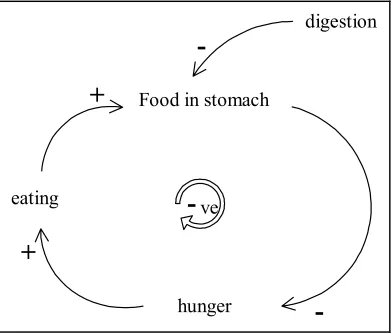
The qualitative aspect of SD was not initially considered to be a very important part of the approach. However in recent years the benefits of focussing on this aspect have been increasingly appreciated [3]. The initial discussion of the problem being modelled works to identify the elements considered fundamental to the system and those that are likely to generate an influence in the problem situation. The identified elements are presented in the form of an influence diagram, an example of which is shown in Figure 1.

Food in stomach

hunger eating

+

+

--ve

digestion

The identified elements are connected by arrows. The “+” and “−” signs denote the direction of the influence, but do not show the magnitude of the influence. For example, as eating increases food in stomach increases, shown by a “+”; as digestion increases,

food in stomach decreases, shown by a “−”. In this way complex and informative diagrams can be built up to represent and clarify the problem being investigated, providing insights into how the variables interact.

In many cases the qualitative analysis of these diagrams is of considerable value in its own right. The aim of this analysis is to find loops, as in the above example, where elements are connected by a directed cycle of arrows. Balanced loops contain an odd number of “−” signs, whereas reinforcing loops or vicious circles contain an even number of “−” signs. The above example, a balanced loop, shows how the system regulates itself. The hungrier we are, the more we want to eat. Eating obviously increases the amount of food in our stomach, but this makes us feel less hungry, so we stop eating. Identifying both types of loop can be very helpful in understanding system behaviour.

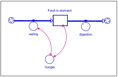
If a quantitative model is to be developed, the influence diagram is converted to a flow diagram. Figure 2 shows the flow diagram for this system in the notation of the software STELLA [4]. This flow diagram has been constructed from the influence diagram shown in Figure 1. The two “clouds” represent a source and a sink, in other words infinite amounts of the material (in this case, food) that flows through the system. The stomach is modelled as a stock or level of food. Eating and digestion are defined as rates, in this case the rates at which food flows into and out of the stomach. Food can flow into or out of a stock according to numerical values defining the rates of eating and digesting.

Hunger is a “soft” variable that can be measured, as opposed to quantified, and can be defined graphically. It is linked to, and therefore influences, the rate at which eating

takes place. The quantity of food in the stomach in turn influences hunger, completing the cycle.

Food in stomach

hunger

eating digestion

Figure 2. Example of a simple model using STELLA notation

St(t+1) = St(t) + eating rate *dt – digestion rate * dt

The time spent in each stage can be modelled by the use of delays. The simplest type of delay is the exponential delay. If for example the average time taken to digest food is 4

time units, the digestion rate is equal to 4

) (t St

. Modern SD software has the facility to

implement more complex types of delay function, such as pipeline delays and batch delays, which permit non-exponential dwelling times in the various stages to be

modelled. However SD undeniably lacks the total flexibility of discrete event simulation, which can use virtually any probability distribution function, or empirical data, to model state dwelling times.

As with most modelling approaches, the process of formulating the problem improves communication and increases understanding of the problem. More tangible outputs are numerical in the form of tables and graphs providing specific data on how the variables are changing with time. In recent years there has been a trend towards SD software that is easy to use and does not require any knowledge of computer programming. STELLA, for example, has a “drag and drop” interface so that the user can select icons for levels, rates, etc, place them on the screen, connect them up, and edit their properties; the software then automatically generates the underlying equations and runs the model, collecting and presenting the output.

3. Applications of system dynamics models

SD models have the capability of using descriptive or judgmental data as well as numerical data. The overall emphasis, particularly of qualitative models, is on policy rather than decisions. SD models are not used for optimisation or point prediction. In fact, Jay Forrester [2] said that SD models are “learning laboratories” and rather more

contentiously, David Lane [5] argued that SD models are never more than 40% accurate.

In a special issue of the Journal of the British Operational Research Society [3] on the theme “System Dynamics for Policy, Strategy and Management Education”, Brian Dangerfield presented a survey of applications of system dynamics to health care issues in Europe [6]. Dangerfield’s own work with Carole Roberts in the field of HIV/AIDS modelling is well known, and their 1990 paper [7] on quantitative SD models for AIDS won the OR Society President’s Medal for its role in increasing public awareness of OR modelling.

was discharged. In theory, this would reduce the number of discharges and would reduce overall social services costs.

+

-

--

+ +

-+

+

Community care budget

Hospital discharge rate

In community care

Community care costs

Hospital waiting list

-In hospital _Hospital

admission rate

+

Funds available

Figure 3. Wolstenholme’s model for community care (after Wolstenholme, [8])

This intended effect is shown in the inner loop of the influence diagram in Figure 3. However the outer loop of this model shows that an (unintended) effect of the

Community Care Act would actually be actually to increase social service spending, since as hospital discharges decrease fewer beds become available, thus limiting admissions, and increasing the number of sick elderly people in the community awaiting admission and requiring costly care at home.

Wolstenholme chose SD because he wished to communicate with politicians and health care planners in order to expose how unintended effects might cause waiting lists to increase. Accurately estimating the actual numbers of patients was less important than gaining an understanding of how the system worked. The model was extended to include other types of residential care and was implemented in an interactive gaming mode.

A more recent example, this time of a quantitative SD model, is Townshend and Turner’s model [9] for screening for Chlamydia, a sexually transmitted infection that is a major cause of infertility in the UK. Chlamydia infection is a good candidate for screening as it is asymptomatic in its early stages yet can still be detected and successfully treated. Townshend and Turner constructed an ithink (STELLA) model of a population stratified by age and by risk group, using subscripted arrays. They chose SD partly because of the large populations in the model, which would make a DES model too cumbersome to run, and partly because of the need to model the feedback effects due to re-infection of treated people, and the reduction in the prevalence of Chlamydia after screening.

and emergency department. SD models developed by ORAHS members include Rauner’s quantitative model for predicting the size of the AIDS epidemic in Austria [12]. These models all handle very large populations.

To summarise, SD models are mainly used at a strategic or conceptual level; they are basically deterministic, and they treat simulated objects as a continuous mass. The aim of an SD model is usually to gain an understanding of feedback dynamics and long-term system behaviour. The models may not be simulated at all since the influence diagrams are often found to be the most useful part of the modelling process. SD does not attempt optimisation or point prediction, but it is capable of modelling very large complex systems and can deliver a wealth of qualitative and quantitative output measures. SD is less good at detailed resource allocation problems. Parameter estimation and validation are less of an issue with SD than with DES (but still difficult). Compared with DES, and with a few notable exceptions, SD models are not all that well-known in the academic community and are not widely used by practitioners.

4. Case study: Hilton’s SD model for cardiac surgery

The case study was developed as an initial stage in Hilton’s doctoral thesis. The model used the SD software STELLA, in order to investigate the long waiting lists known to exist for NHS patients requiring cardiac surgery.

In the model, patients suffering from coronary artery disease were referred to a cardiac surgeon who clinically assessed them. If they were considered suitable for Coronary Artery Bypass surgery, they were then placed on a waiting list. There were three types of waiting list, depending on the severity of disease. Patients could switch between waiting lists and could also come into the system as emergency admissions.

In the model, the number of patients who could be treated per annum was governed by the contract level. The contract level is a fixed number of operations that the local Health Authority agrees (annually in advance) to buy from the providing hospitals. It was

assumed that surgery was carried out on a “worst-come-first-served” basis, so patients considered to have the greatest clinical need were treated first.

The aims of this early model were

• to identify the influences acting on the waiting lists; • to improve understanding of the dynamics of the lists; • to investigate how the lists interact with each other.

throughput costs Waiting list length Patients requiring reassessment Patients upgraded Length of stay /

care required cancellations + + + + + + + _ _ _ throughput costs Waiting list length Patients requiring reassessment Patients upgraded Length of stay /

care required cancellations + + + + + + + _ _ _

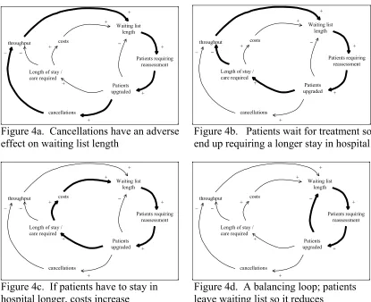
Figure 4a. Cancellations have an adverse Figure 4b. Patients wait for treatment so effect on waiting list length end up requiring a longer stay in hospital

throughput costs Waiting list length Patients requiring reassessment Patients upgraded Length of stay /

care required cancellations + + + + + + + _ _ _ throughput costs Waiting list length Patients requiring reassessment Patients upgraded Length of stay /

care required cancellations + + + + + + + _ _ _

Figure 4c. If patients have to stay in Figure 4d. A balancing loop; patients hospital longer, costs increase leave waiting list so it reduces

From this influence diagram a representation of the basic structure of the cardiac system was devised, as shown in Figure 5. This schematically represents the possible pathways for patients to follow, after they have presented with cardiac symptoms and been referred for a surgical consultation.

D E C I S I O N T R E A T M E N T Routine WL Urgent WL Unstable WL Emergency Patient passage

Figure 5. Schematic representation of Cardiac waiting lists of different priorites.

routine urgent unstable emergency no routine no urgent no unstable no emergency rate on routine

rate on urgent

rate on unstable

rate on emergency

rate off routine

rate off urgent

rate off unstable

rate off emergency x

y

z

maximum no pts contract level

rate off emergency rate off unstable

upgrade R to Uns upgrade R'

upgrade R to Ur

upgrade Ur to Uns

upgrade Uns to Em upgrade R

upgrade Ur

upgrade Uns

In Figure 5, following a decision made by the surgeon, and assuming that the patient is considered suitable for surgery, the patient is placed on a waiting list either as a routine, urgent or unstable patient.

Based on the simple diagram a system dynamics flowchart was constructed to enable the model to be completed. The waiting lists have been considered to be a stock of patients with the valves that determine the input and output of the waiting lists to be the referral rate and the admission rate in each case. The SD diagram is shown in Figure 6.

Quantitative data were required in order to complete the model and allow it to run. This was gathered from surgeons and databases in a large teaching hospital. Several

simulations were run altering, systematically, the variables and the results analysed, some of which are presented here.

0 50 100 150 200 250 300 350

600 700 800 900 1000 1100 1200

contract level no r outi ne p at ie nt s 0 20 40 60 80 100 120

600 700 800 900 1000 1100 1200

contract level no em er ge nc y p at ien ts

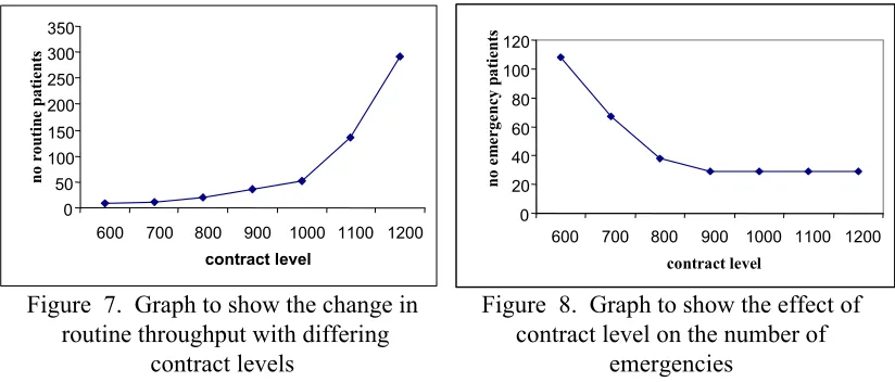
Figure 7. Graph to show the change in routine throughput with differing

contract levels

Figure 8. Graph to show the effect of contract level on the number of

emergencies

Figure 7 shows that as contract levels increase, so does the number of routine patients who are treated. At very low contract levels, the number of treatments available is only just sufficient to cope with the unstable and urgent patients. In this scenario almost no routine patients can be scheduled for treatment as routine patients, and they are only treated when their condition deteriorates and they are reclassified as unstable or

emergency. As more treatments become available, more routine patients can be treated directly from the routine waiting list and not following an “upgrade” due to a change in clinical status.

Figure 8 shows that the effect of the contract level on the number of emergency patients requiring admission is considerable. An insufficient contract level puts pressure on the waiting lists. Patients wait a long time for treatment as throughput is limited. As the disease suffered by the patient advances the likelihood of the patient coming to hospital as an emergency is increased, leading to an increased number of emergency admissions.

levels progressing to a point where an emergency admission is necessary, but some patients will only realise that treatment is required following a severe heart attack.

System dynamics was used in this model since the focus of the study was not to follow individual patients around the system, but to look at the behaviour of certain aspects of the system. No attempt was to be made to optimise the running of the cardiac system. However, an understanding of how the system as a whole reacted to changes in, for instance, contract policy, was to be gained. In addition SD allowed qualitative factors to be considered in the construction of the influence diagram.

Further study is currently being carried out, expanding the system observed here to include other stages of the cardiac pathway, that is General Practitioners and

Cardiologists. This will enable additional understanding to be gained about how different waiting lists interact across a medical/surgical interface.

5. The basic elements of discrete event simulation

DES is arguably the most widely used OR technique in practice. It is used to model systems that can be viewed as a queueing network. Individual objects (entities) pass through a series of activities, in between which they wait in queues. The rules governing the order in which these activities occur and the conditions for them to take place can be extremely complex. Each individual entity can be given characteristics that determine what happens to that individual in the system. The durations of the activities are usually sampled from probability distribution functions. The modeller has almost unlimited flexibility in the choice of these functions and the logic governing the flow of entities around the system.

DES models make frequent use of animation and graphics, and can be made interactive; all these features are very useful for communication with clients. The models produce a vast range of output, often showing the whole distribution of possible outcomes in addition to summary measures. However each simulation run or iteration only represents one realisation of the system (one possible outcome), and highly variable systems require many iterations. Reducing the variance of the simulation results can be extremely

important, and the interpretation of results needs care. Model validation is an important issue because of the quantitative nature of the results.

DES models have traditionally been applied at a tactical, operational level. They are by definition stochastic in nature and deal with distinct entities, scheduled activities, queues and decision rules. DES models are simulated in unequal timesteps (when “something happens”); the model is almost always simulated, and DES requires large amounts of quantitative, numerical data. The aim of these models is often comparison of scenarios, prediction, or optimising specified performance criteria.

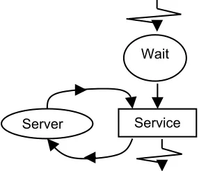
and rectangles. An example of a simple activity diagram is shown in Figure 9. The circle “Wait” is a queue, and the rectangle “Service” is an activity requiring the resource

“Server”. Customer entry and exit points in the system are shown by zigzag lines.

Wait

Service Server

Figure 9. Activity diagram for a simple queueing system

As with SD software, the increase in power and availability of PC’s has led to a trend towards user-friendly and cheap DES software. The advantages are obvious – it is easy to develop a rough working model very quickly, no knowledge of programming is required, and it facilitates communications with clients if the modeller can develop and run a demonstration model during a single meeting. A well-known example of this type of software is SIMUL8 [13]. However these packages need to be handled with care; the simulation results need intelligent analysis by people with some knowledge of statistics, as it is easy to draw disastrously wrong conclusions. The software does have its

limitations – it can be too rigid, and it can be difficult to model simultaneous or interrupted activities, or complex logical rules. For some situations, for example in academic research or for unusual complex systems, the only solution may be to write the simulation from scratch in a programming language such as C++ or Pascal. This of course can be expensive and time-consuming.

6. Applications of discrete event simulation models

The relative dominance of DES over SD in practice is reflected by the vast number of health care applications of DES, compared with SD. Examples abound in the literature in a very wide range of application areas. A recent survey paper by Jun et al [14] contained 117 references for clinic models alone. Examples of models by members of the ORAHS Working Group include Davies and Brailsford’s model for screening for diabetic

retinopathy [15], Riley’s model of Accident and Emergency departments [16], Shahani et al’s hospital capacity model [17], and Davies’ renal transplant model [18]. Davies and Davies [19] argue that DES is the technique of choice for modelling health care systems, which are characterised by variability, uncertainty, and complexity.

amounts of data. Validation can be difficult. Many DES models are well-known in the academic community, yet are still not always widely used in practice; the reasons for this are not clear.

7. Case study: Brailsford’s DES model for AIDS

This model was developed as part of Brailsford’s MSc dissertation [20]. The model used an early version of Davies and O’Keefe’s PASCAL_SIM [21] and was coded in Pascal. The model simulated a population of male homosexuals, including recruitment of new individuals, and was basically driven by a “natural history” model of the progression of HIV infection in an individual. The model also included resource use and transmission of the virus.

In the model, the number of new cases caused by an infected individual depended on three things; the proportion of susceptible (HIV-negative) men in the population, the average number of different sexual partners the infected individual has per unit time, and the probability that a contact between that infected individual and an HIV-negative man would result in a new infection. This probability, known as the force of infection, depended on the clinical status of the infected individual.

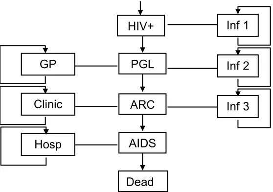
The natural history model contained five clinical states, shown in Figure 10, in increasing degrees of severity: HIV+, Persistent Generalised Lymphadenopathy (PGL), AIDS Related Complex (ARC), AIDS, and Dead. Individual differences in sexual behaviour were modelled by sampling the average number of sexual partners each individual had per annum from a negative exponential distribution. Evidence [22] showed that there is considerable variation between individuals; a few high-risk individuals have a large number of partners, but the majority of individuals have a small number of different partners. Figure 5 also shows how clinical progression is linked to resource use and viral transmission. A very limited set of resources was used: GP time, hospital out-patient visits and hospital bed utilisation. Clinical status was known to affect the viral transmission rate. Infectivity is high in the early stages of infection, but then falls and only rises again just before the onset of clinical AIDS.

This was a very detailed model requiring the estimation of many unknown parameters. One technical difficulty, the modelling of simultaneous activities (clinical progression, consumption of resources and infecting other people) was overcome by the use of

Inf 3 Inf 2 Inf 1

Hosp Clinic

GP

Dead AIDS

ARC PGL HIV+

Figure 10. Three parallel processes in the AIDS simulation

DES was selected as a modelling technique because of the need to track individuals through the system, and to capture the considerable variation between individuals. Variability in sexual behaviour is known to be a critical variable affecting the spread of the epidemic [24]. There were relatively few HIV+ cases compared with the total population, so large numbers were not a problem. Some activities were of very short duration, for example GP visits, whereas the clinical transition times were very long. Lack of data was inevitably a problem, partly due to the time constraints of the MSc dissertation, and the data used were mainly a combination of hypothetical data plus expert medical opinion. The model output consisted of the numbers in each clinical state, plus resource utilisation. The model was further developed over the next three years in Brailsford’s PhD thesis [25].

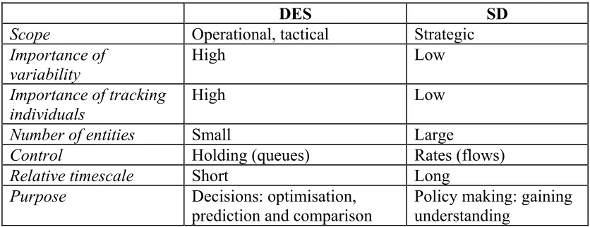
8. The crucial question: which is better?

How do you choose which method to use? Are some systems “naturally” better modelled by SD or by DES … and if so, why? Does the choice of technique simply depend on the personal preference of the modeller, because people tend to stick to what they know best and feel most comfortable with? The answers may depend less on the system being modelled, than on the purpose of the model: what sort of questions do we want our model to answer?

DES SD

Scope Operational, tactical Strategic

Importance of variability

High Low

Importance of tracking individuals

High Low

Number of entities Small Large

Control Holding (queues) Rates (flows)

Relative timescale Short Long

Purpose Decisions: optimisation, prediction and comparison

Policy making: gaining understanding

Table 1. Criteria for selection of modelling approach

For example, suppose the system under consideration is a hospital out-patients clinic. We might choose SD if we are looking at the clinic in a broad context, and we are interested in its interaction with other parts of the hospital or the community health service; if all patients are roughly similar in behaviour; if there are large numbers of patients; if we want qualitative output (for example why certain clinics overrun, and how this affects discharges from surgical wards); and if we have a timescale of weeks, months or years.

On the other hand, we might choose DES if we are looking at the clinic in a narrow context, and there is little contact with the outside world; if individual patients differ considerably in behaviour; if there are relatively small numbers of patients; if we want quantitative output (patient waiting times, resource utilisation, etc); if we want to compare scenarios, for example different staffing levels; and if we have a timescale of hours or days.

Two comparisons in the literature are of interest in this context. It should be pointed out that both comparisons were made by afficionados of SD, and that the earlier comparison by Randers [26] was not a direct comparison between SD and DES, but between SD and quantitative modelling approaches in general. The authors are grateful to David Lane for bringing the Randers’ comparison to their attention. The technological developments in computer hardware and software since 1980, when Randers made his comparison, also affect the validity of this comparison today.

DES SD Point predictive

ability

Formal

correspondence with data

Fertility

Ease of enrichment

Relevance (usefulness) Transparency

Mode reproduction ability Insight generating

capacity _{Descriptive realism}

Figure 11. Randers’ comparison (after Randers [26])

The keenest proponent of SD would have to admit that DES is superior in the areas of

formal correspondence with data and point predictive ability, although in fairness SD does not attempt to compete here. In the authors’ view, both approaches can be equally

useful and relevant if used appropriately, although DES has actually been used more widely than SD.

DES SD

Perspective Analytic, emphasis on detail

complexity Holistic, emphasis on dynamic complexity

Resolution Individual entities, attributes, decisions and events

Homogenised entities, continuous policy pressures and emergent behaviour

Data sources Numerical with some judgmental elements

Broadly drawn

Problems studied

Operational (?) Strategic (?)

Model elements

Physical, tangible plus some information

Physical, tangible, judgmental and information links

Human agents Decisions Policies

Clients find the

model Opaque, “dark grey box”: convincing Transparent, “Fuzzy glass box”; compelling

Outputs Point predictions, performance measures

Understanding of structural source of behaviour modes

Table 2. Lane’s comparison (due to Lane [27])

In Lane’s experience clients find SD models compelling; he believes they are excited by SD models whereas they find DES models more mundane (although convincing). It should be borne in mind that Lane is a proponent of SD, and users of DES might well argue that their clients have found their models both exciting and convincing! However Lane calls for closer links between the two communities of modellers, which can only be of mutual benefit.

9. Conclusion

We have attempted to give an overview of discrete event simulation and system dynamics, to describe the strengths and weaknesses of each approach in (hopefully) an unbiased way, and to offer some guidelines to potential users about the selection of an appropriate technique for a given problem. We echo David Lane’s opinion that more communication and discourse between the communities of SD and DES modellers would have great benefit, particularly in the field of health care.

References

1. J.W. Forrester. Industrial Dynamics. MIT Press, Cambridge, MA (1961), reprinted by Productivity Press (1994) and now available from Pegasus Communications,

Waltham, MA, USA.

2. J.W. Forrester. The impact of feedback control concepts on the Management

3. Special issue on System Dynamics for Policy, Strategy and Management Education.

Journal of the Operational Research Society, 50, No. 4, April 1999.

4. STELLA, High Performance Systems, 45 Lyme Road Suite 300, Hanover NH 03755 http://www.hps-inc.com/.

5. D.C. Lane. You just don't understand me: Modes of failure and success in the discourse between system dynamics and discrete event simulation. LSE OR Dept Working Paper LSEOR 00-34, London School of Economics and Political Science, 2000.

6. B.C. Dangerfield. System dynamics applications to European health care issues.

Journal of the Operational Research Society, 50, pp 345-353, 1999.

7. B.C. Dangerfield and C.A. Roberts, Modelling the epidemiological consequences of HIV infection and AIDS: a contribution from operational research. Journal of the Operational Research Society, 41, pp 273-289, 1990.

8. E.F. Wolstenholme. A case study in community care using systems thinking. Journal of the Operational Research Society, 44, pp 925-34, 1993.

9. J.R.P. Townshend and H.S. Turner. Analysing the effect of Chlamydia screening.

Journal of the Operational Research Society, 51, pp 812-24, 2000.

10. R.G. Coyle. A systems approach to the management of a hospital for short-term patients. Socio-Economic Planning Science, 18, pp 219-226, 1984.

11. D.C. Lane, C. Monefeld and J.V.Rosenhead. Looking in the wrong place for healthcare improvements: a system dynamics study of an accident and emergency department. Journal of the Operational Research Society, 51, pp 518-531, 2000.

12. M.S.Rauner. Managing the AIDS epidemic in Vienna, Austria: prevention strategies for the 21st century, in: Information, management and planning of health services, Proceedings of the 25th meeting of the European Working Group on Operational Research Applied to Health Services, Valmiera, Latvia, July 18-23, 1999, ed. E. Mikitis (Health Statistics and Medical Technology Agency, Riga, Latvia, 2000).

13. SIMUL8 Corporation, 141 St James Road Glasgow G4 0LT, Scotland, www.simul8.com.

14. J.B. Jun, S.H. Jacobson and J.R. Swisher. Application of discrete-event simulation in health care clinics: A survey. Journal of the Operational Research Society, 50,

pp109-123, 1999.

15. R. Davies, S.C. Brailsford, P.J. Roderick, C.R. Canning and D.N. Crabbe. Using simulation modelling for evaluating screening services for diabetic retinopathy.

16. J. Riley. Visual interactive simulation of accident and emergency departments. In:

Managing Health Care Under Resource Constraints. Proceedings of the 21st Annual Meeting of the ORAHS EURO-WG, Eindhoven University Press, Netherlands, 1996.

17. J.C. Ridge, S.K. Jones, M.S. Nielsen, and A.K. Shahani. Capacity planning for intensive care units. European Journal Of Operational Research,105, pp 346-355, 1998.

18. R .Davies and H. Davies. A simulation-model for planning services for renal patients in Europe. Journal of the Operational Research Society, 38, pp 693-700, 1987.

19. R .Davies and H. Davies. Modelling patient flows and resource provision in health systems. Omega, 22, pp. 123-131.

20. S.C. Brailsford. MSc dissertation, Faculty of Mathematical Studies, University of Southampton, 1988.

21. R.Davies and R.M. O’Keefe. Simulation Modelling with Pascal. Prentice Hall, London (1989).

22. C.A.Carne, W.V.D.Weller, A.M.Johnson et al. Prevalence of antibodies to Human Immunodeficiency Virus, gonorrhea rates, and changed sexual behaviour in homosexual men in London. The Lancet, i, pp 656-658, 1987.

23. K.D. Tocher. The Art of Simulation. English Universities Press, London, 1963.

24. R.M.Anderson, G.F.Medley, R.M.May and A.M.Johnson. A preliminary study of the transmission dynamics of the Human Immunodeficiency Virus (HIV), the causative agent of AIDS. IMA J. Math. Appl. Med.Biol., 3, pp 229-283, 1986.

25. S.C. Brailsford. PhD dissertation, Faculty of Mathematical Studies, University of Southampton, 1993.

26. J. Randers (ed). Elements of the System Dynamics Method. MIT Press, Cambridge, MA. 1980.