Free-form modelling of galaxy clusters: a Bayesian and data-driven
approach
Malak Olamaie,
1,2‹Michael P. Hobson,
2Farhan Feroz,
2Keith J. B. Grainge,
2,4Anthony Lasenby,
2,3Yvette C. Perrott,
2Clare Rumsey
2and Richard D. E. Saunders
2,31Imperial Centre for Inference and Cosmology (ICIC), Imperial College, Prince Concort Road, London SW7 2AZ, UK
2Astrophysics Group, Battcock Centre for Experimental Astrophysics, Cavendish Laboratory, 19 J. J. Thomson Avenue, Cambridge CB3 0HE, UK 3Kavli Institute for Cosmology Cambridge, Madingley Road, Cambridge CB3 0HA, UK
4Jodrell Bank Centre for Astrophysics, School of Physics and Astronomy, Alan Turing Building, Oxford Road, Manchester, M13 9PL, UK
Accepted 2018 August 30. Received 2018 August 28; in original form 2017 May 30
A B S T R A C T
A new method is presented for modelling the physical properties of galaxy clusters. Our tech-nique moves away from the traditional approach of assuming specific parameterized functional forms for the variation of physical quantities within the cluster, and instead allows for a ‘free-form’ reconstruction, but one for which the level of complexity is determined automatically by the observational data and may depend on position within the cluster. This is achieved by rep-resenting each independent cluster property as some interpolating or approximating function that is specified by a set of control points, or ‘nodes’, for which the number of nodes, together with their positions and amplitudes, are allowed to vary and are inferred in a Bayesian manner from the data. We illustrate our nodal approach in the case of a spherical cluster by mod-elling the electron pressure profilePe(r) in analyses both of simulated Sunyaev–Zel’dovich (SZ) data from the Arcminute MicroKelvin Imager (AMI) and of real AMI observations of the cluster MACS J0744+3927 in the CLASH sample. We demonstrate that one may indeed determine the complexity supported by the data in the reconstructedPe(r), and that one may constrain two very important quantities in such an analysis: the cluster total volume integrated Comptonization parameter (Ytot) and the extent of the gas distribution in the cluster (rmax). The approach is also well-suited to detecting clusters in blind SZ surveys, in the case where the population of radio sources is known in advance.
Key words: methods: data analysis – galaxies: clusters – cosmology: observations.
1 I N T R O D U C T I O N
Determining the properties of clusters of galaxies, such as their total and baryonic mass, has the potential to provide an independent tool for constraining the parameters of theCDM model, since cluster population properties are sensitive to several cosmological parameters, most notablyσ8(see, e.g. Sievers et al.2013, Planck
Collaboration et al.2016, and de Haan et al.2016). The challenge lies, however, in obtaining a robust estimate of the cluster masses, as these are not directly observable. The mass distribution within a cluster is usually measured with a variety of observational methods, including X-ray (see, e.g. Vikhlinin et al.2009, Ettori2013, Mantz et al.2014,and Olamaie et al.2015), the Sunyaev–Zel’dovich (SZ) effect (see, e.g. Hasselfield et al.2013; Planck Collaboration et al.
2013, Schammel et al.2013, Perrott et al. 2015, Rumsey et al.
E-mail:[email protected]
2016, and Rodr´ıguez-Gonz´alvez et al.2017), measurement of line-of-sight velocity dispersions of the galaxies in a cluster (see, e.g. Rines et al.2010, Munari et al.2013, Saro et al.2013, and Sif´on et al.2013), and gravitational lensing (see, e.g. Rozo et al.2010, Hoekstra et al.2013, Rozo et al.2014and Battaglia et al.2016).
Each of these approaches relies on developing some method for determining the cluster’s mass (distribution) from its observ-able properties, namely its distributions of X-ray surface bright-ness, SZ Comptonization parameter, line of sight velocity disper-sions, and weak-lensing shear distribution. This is usually achieved by modelling the physical properties through the cluster in terms of some specific parameterized functional forms. Typical exam-ples include assuming an NFW profile (Navarro, Frenk & White
1996, 1997) for the dark matter density distribution, a β-model (Cavaliere & Fusco-Femiano 1976, 1978) for the gas density, or a generalised NFW (GNFW) profile (Nagai et al. 2007) for the gas pressure. The cluster mass (distribution) is then usually calculated under the standard assumption of a spherical cluster
model obeying hydrostatic equilibrium (HSE) and/or some scaling relationships.
Even for physically based cluster models (see, e.g. Olamaie, Hobson & Grainge2012, 2013), there still remains considerable uncertainty regarding the appropriate form one should assume for the radial variation of cluster properties, and this can lead to differ-ent cluster mass estimates (see, e.g. Olamaie et al.2012, Giodini et al.2013, and K¨ohlinger, Hoekstra & Eriksen2015, and De Mar-tino & Atrio-Barandela2016). This may result from either adopting inappropriate functional forms, often by extrapolating their use to cluster masses and/or redshifts that are not well sampled by observa-tions or simulaobserva-tions, or by fitting models that depend on parameters to which the data are insensitive.
In this paper, we therefore move away from the traditional ap-proach of assuming specific parameterized forms for the variation of cluster properties, such as the pressure, density, and/or temperature distribution, and instead allow for a ‘free-form’ reconstruction, but one for which the level of complexity is determined automatically by the observational data and may depend on position within the cluster. This is achieved by representing each independent cluster property as some interpolating or approximating function (for ex-ample, a piecewise linear interpolation or a spline) that is specified by a set of control points, or ‘nodes’. The positions and amplitudes of these nodes and, most importantly, the number of nodes used are allowed to vary and constitute the set of parameters to be inferred from the data in a Bayesian manner.
We note that we have already successfully applied such a Bayesian nodal modelling approach to a number of cosmological analysis problems, including the reconstruction of the primordial anisotropy power spectrum and the variation of the dark energy equation-of-state parameter with redshift (see, e.g. V´azquez et al.
2012a,b and Hee et al.2016,2017).
The structure of this paper is as follows. In Section 2, we briefly summarize Bayesian inference, in particular parameter estimation and model selection. Our nodal approach to modelling galaxy clus-ters is presented in Section 3, and in Section 4 we apply it to the particular case of modelling the pressure profilePe(r) in a spherical
cluster observed via its SZ effect. Section 5 outlines our Bayesian methodology for inferring the cluster parameters from interfero-metric SZ observations, and summarizes our simulated cluster ob-servations and real obob-servations of the cluster MACS J0744+3927 using AMI. In Section 6, we present the results of our Bayesian nodal analysis of these simulations and real observations, and we conclude in Section 7.
2 B AY E S I A N I N F E R E N C E
For the analysis of some data D in the context of a model (or hypothesis)Mthat depends on some set of parameters, Bayes’ theorem states that
Pr(|D,M)= Pr(D|,M) Pr(|M) Pr(D|M) ≡
L()π()
Z , (1)
which is usually interpreted as the prior probability distribution Pr(|M)≡π() of the parameters being updated by the likeli-hood Pr(D|,M)≡L() of obtaining the observed data given some set of parameter values to yield the posterior probability dis-tribution Pr(|D,M) of the parameters, which is normalized by the Bayesian evidence Pr(D|M)≡Z(which does not depend on the parameters). The joint (unnormalizsed) posterior provides the complete inference in Bayesian parameter estimation, and can be
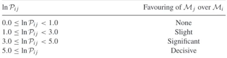
Table 1. Jeffreys’ scale for interpreting PORs (or Bayes factors). As lnPij= −lnPj i, negative values imply reversed model favouring.
lnPij Favouring ofMjoverMi
0.0≤lnPij<1.0 None
1.0≤lnPij<3.0 Slight
3.0≤lnPij<5.0 Significant
5.0≤lnPij Decisive
subsequently marginalized over each parameter to obtain individual parameter constraints.
Similarly, in Bayesian model selection, one can calculate the probability of a model given the data as
Pr(M|D)= Pr(D|M) Pr(M) Pr(D) ≡
ZπM
Pr(D). (2)
Taking the ratio of the probabilities of two models signifies our degree of belief in one model over another, and is given by the posterior odds ratio (POR)
Pij ≡ Pr(Mj|D) Pr(Mi|D) = ZjπMj ZiπMi =Bij πMj πMi , (3)
whereBij ≡Zj/Ziis the Bayes factor (Jeffreys1961). Clearly, if
πMj =πMi, so that the two models are considereda prioriequally probable, then Pij =Bij. Table 1lists a modern version of
Jef-freys’ criteria, which are used to give meaning to this quantification (Kass & Raftery1995; Feroz2013).
Thus, for Bayesian model selection, in contrast to parameter esti-mation, the evidence takes a central role. Typically, the evidence for each model is calculated separately and their ratios evaluated. From (1), the evidence is the normalization constant for the posterior, which is given by
Z=
L()π() dD , (4)
whereDis the dimensionality of the parameter space. As the average of the likelihood over the prior, the evidence embodies the notion of Occam’s razor (see, e.g, Jaynes1986and Sivia2005): a simple theory with a compact parameter space will have a larger evidence than a more complicated one, unless the latter is significantly better at explaining the data.
The evaluation of the multidimensional integral (4) over the whole parameter space is a challenging numerical task. We perform this calculation here using the nested sampling algorithm MULTI-NEST (Feroz & Hobson 2008; Feroz, Hobson & Bridges2009; Feroz et al.2013). This Monte-Carlo method is targeted at the effi-cient calculation of the evidence, but as a by-product also produces posterior inferences for parameter estimation; it is also very ef-ficient at exploring posteriors that contain multiple modes and/or large (curving) degeneracies.
We note that elsewhere (Hee et al.2016,2017), we have presented an alternative method for performing Bayesian model selection, without explicitly computing evidences, which uses a combined likelihood and introduces an integer model selection parametern. If the maximum number of models under consideration is specified
a priori, the full joint parameter space of the models is of fixed dimensionality and can be explored using standard sampling meth-ods, without the need for trans-dimensional techniques, although the posterior is usually highly multimodal and hence nested sam-pling is again an obvious choice. Bayes factors, or more generally posterior odds ratios, may then be read off directly from the poste-rior onn, which is obtained by straightforward marginalization. To
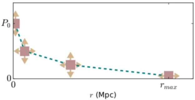
Figure 1. Linearly-interpolated nodal representation forN=4 nodes of the gas pressure profilePe(r) in a galaxy cluster described in units of MeVm−3
(1MeVm−3=1.602×10⁻¹³Nm−2).
keep our discussion simple, however, we will not use this method here, but plan to apply it to nodal modelling of galaxy clusters in a forthcoming publication.
In closing this section, it should be mentioned that, in general, a gain in information via a Bayesian analysis may be achieved in several ways: it can occur because of a tightening of the pa-rameter constraints, a shift in position of the peak(s) of the dis-tribution from prior to posterior, or an increase in the evidence (see, e.g. Trotta et al. 2008, Seehars et al. 2014, and Seehars et al.2016).
3 N O DA L M O D E L F O R A G A L A X Y C L U S T E R
As described briefly earlier, in our nodal approach to free-form modelling of a galaxy cluster, each independent physical property of the cluster is represented by some interpolating or approximating function that is determined by a set of control points, or nodes. In principle, these functions can be fully three-dimensional, such that
fi=fi(r,θ,φ, . . . ) for some set of functions, to allow modelling
of arbitrary structure in each property of interest in the cluster. To illustrate the method simply, however, we will consider here the special case of a spherical cluster, such that each property is a function only of radiusrfrom the cluster centre. Moreover, we will specialize still further to the case where one constructs a nodal model of just a single property of interest, described by some functionf(r). It is a straightforward matter to extend the following analysis to multiple properties of interest.
The basic idea is to representf(r) not with some standard pa-rameterized functional form, as in most current cluster analyses, but in terms of a numberNof nodes in (r,f)-space, separated by their corresponding positionsrnand amplitudesfn(n=0, 1, 2, . . . , N−1) (thus each node can ‘move’ both horizontally and vertically – see Fig.1), whereNis itself determined in the analysis (or, in principle, marginalized over). TheNnodes act as control points for the continuous functionf(r). In this way, one obtains a continuous free-form reconstruction of the profilef(r), for which the complexity is regularized by the data under analysis.
One is free to choose from a wide range of possible interpolation or approximation methods, such as a constant function between the nodes, polynomials, rational functions, splines, B´ezier curves, or even Gaussian processes. It should be noted, however, that some forms of smooth interpolating or approximating functions, such as cubic splines, have continuity requirements on the function and its derivatives which can significantly reduce the ability of the result-ingf(r) to reproduce abrupt features in the cluster profile (V´azquez et al.2012). We also note that assuming a function that is constant between the nodes breaks the continuity requirement of the pressure
profile. In principle, the nature of the interpolating or approximat-ing function could be determined by performapproximat-ing a straightforward Bayesian model selection between the various options, although we will not consider that further here. Instead, for illustration, we choose here the simplest approach of linearly interpolating between the nodes; since we are performing an interpolation, rather than an approximation, one hasfn=f(rn).
As mentioned above, given the nature of the one-dimensional functionf(r) that we wish to model in the case of a galaxy cluster, we typically restrict the movement of the first and last nodes (or end nodes) as follows. The first node has a fixed position, at the origin, such thatr0 =0. Consequently, its corresponding
ampli-tude parameterf0represents the central valuef(0), which is often
of interest in galaxy cluster analyses. To determine the impact of this restriction, however, which assumes knowledge of the position of the cluster centre, we also study the case where the position of the first node is not fixed. In contrast, the last node has a fixed amplitude of zero, such that fN−1 = 0. Thus, its corresponding
position parameter rN−1can sometimes be interpreted as an
ex-tent of the clusterrmax, which is again often of interest (although
this interpretation does depend on the nature of the quantityf(r) being modelled). In our demonstration of the method presented in Section 4,f(r) represents the electron pressure profilePe(r) of the
cluster and sorN−1represents the extent of the cluster gas. Fig.1
illustrates our linearly interpolated nodal model ofPe(r) forN=4
nodes.
In the context of Bayesian inference, we denote the model con-sisting ofNnodes byMN, which has the parameters={rn,fn}
forn=0, 1, 2, . . . ,N−1, plus any further ‘global’ parameters, such as the cluster position on the sky or parameters describing any contaminating signals or noise in the data. The priors on the parameters may be chosen to accommodate whatever information is availablea priori. In general, however, we typically also impose a ‘sorting condition’ on the node positions, such thatrn<rn+ 1. This
can be done straightforwardly, without the need to reject any sam-ples. Indeed, if each node position is considered to be drawn from a uniform distribution in some given range, as is usually the case, the corresponding (non-separable) joint priorπ(r0,r1,r2, . . . ,rN−1)
on the node positions, which incorporates the sorting conditionrn
<rn+ 1, has an analytic form in terms of the beta distribution
(Han-dley, Hobson & Lasenby2015). It is also worth mentioning that, although we will assume here that each modelMNis equally likely a priori, such thatπMi =πMj (and hence PORs are equivalent to Bayes factors), this is not necessary. One may view this assumption as imposing a uniform prior (within some range) on the numberN
of nodes, but one could equally well impose, for example, a Poisson prior onNwith some given mean, from which one can read off the corresponding values ofπMN.
In the straightforward model selection approach used here, one begins by analysing the N = 2 model, using MULTINEST to calculate the evidenceZ2and obtain samples from the posterior Pr(|D,M2). This process is then repeated separately forN=3, 4, . . . until the evidenceZNhas decreased well below that of the
most-favoured model. One may then proceed either by conditioning on the most-favoured modelMNˆ and simply infer parameters and the
corresponding constraints onf(r) from the posterior Pr(|D,MNˆ)
or perform a ‘multi-model’ inference (see e.g. Parkinson & Lid-dle 2013, Hee et al.2016,2017, and Planck Collaboration et al.
2016) in which the constraints onf(r) are determined by averag-ing over all the modelsMN considered, weighted by their PORs.
In the interests of simplicity we will adopt the former approach here.
4 A P P L I C AT I O N T O S Z O B S E RVAT I O N S
Although our nodal approach may be used to model observations of galaxy clusters in any waveband, we illustrate the method here by applying it to SZ observations (see e.g. Sunyaev & Zeldovich1970, Birkinshaw1999, and Carlstrom, Holder & Reese2002). Since the SZ surface brightness is proportional to the line-of-sight integral of the electron pressure, as we show below, it is natural to use the nodal approach to model the radial electron pressure profilePe(r)
of the ionized gas within the cluster.
The observed SZ surface brightness δIν in the direction of an
electron reservoir is given by
δIν=TCMByf(ν) ∂Bν ∂T T=TCMB . (5)
Here, Bν is the blackbody spectrum, TCMB = 2.73 K (Fixsen
et al. 1996) is the temperature of the CMB radiation, f(ν)= (xcoth(x/2)−4) (1+δ(x, Te)) is the frequency dependence of
thermal SZ signal,x= hpν
kBTCMB,hpis Planck’s constant,νis the fre-quency, and kBis Boltzmann’s constant. The functionδ(x,Te) takes
into account the relativistic corrections in the study of the thermal SZ effect which is due to the presence of thermal weakly relativistic electrons in the ICM and is derived by solving the Kompaneets equa-tion up to the higher orders (Rephaeli1995, Challinor & Lasenby
1998, Itoh, Kohyama & Nozawa1998, Nozawa, Itoh & Kohyama
1998, Pointecouteau, Giard & Barret1998). It should be noted that at 15 GHz (AMI observing frequency)x=0.3 and therefore the relativistic correction, as shown by Rephaeli (1995), is negligible forkBTe≤15 keV. The dimensionless parametery, known as the
Comptonization parameter, is the integral of the number of colli-sions multiplied by the mean fractional energy change of photons per collision, along the line of sight
y= σT mec2
+∞ −∞
Pe(r) dl , (6)
wherePe(r) is the electron pressure at radiusr, respectively,σTis
Thomson scattering cross-section,meis the electron rest mass,cis
the speed of light, anddlis the line element along the line of sight. It should be noted that (6) assumes an ideal gas equation of state.
The integral (YSZ) of the Comptonizationyparameter over the
solid anglesubtended by the cluster is proportional to the volume integral of the gas pressure. It is thus a good estimate for the total thermal energy content of the cluster and hence its mass (see e.g. Bartlett & Silk1994). TheYSZparameter in cylindrical and spherical
geometries, respectively, may be described as
Ycyl(R)= σT mec2 +∞ −∞ dl R 0 Pe(r)2π sds , Ysph(r)= σT mec2 r 0 Pe(r)4π r2dr, (7)
whereR is the projected radius of the cluster on the sky. Thus, by using our nodal approach to modelPe(r), one may constrain YSZin either geometry. In this paper, we calculate the marginalized
posterior distribution of the cluster total volume integrated Comp-tonization parameter,Ytot=Ysph(rmax), wherermaxis the extent of
the cluster.
5 A N A LY S I S O F I N T E R F E R O M E T R I C S Z DATA
In order to verify that our proposed model, with its correspond-ing assumptions, can describe profiles of cluster physical properties accurately, we carry out a Bayesian analysis of simulated SZ obser-vations using AMI (AMI Consortium: Zwart et al.2008) of a set of
three clusters, as well as real AMI SZ observations of the cluster MACS J0744+3927 (Rumsey et al.2016).
5.1 Bayesian methodology
An interferometer like AMI operating at a frequencyν measures samples from the complex visibility plane ˜Iν(u). These are given
by a weighted Fourier transform of the surface brightness Iν(x),
namely ˜
Iν(u)=
Aν(x)Iν(x) exp(2π iu·x) dx, (8)
wherexis the position on the sky relative to the phase centre,Aν(x)
is the (power) primary beam of the antennas at observing frequency
ν(normalized to unity at its peak), anduis the baseline vector in units of wavelength.
Details of our Bayesian methodology for modelling interfero-metric SZ data, primordial CMB anisotropies, and resolved and unresolved radio point-source are given in Hobson & Maisinger (2002), Feroz & Hobson (2008), Feroz et al. (2009), AMI Consor-tium: Davies et al. (2011) and AMI Consortium: Olamaie M. et al. (2012).
In short, the measured interferometer visibilities in our model are assumed to have the form
Vν(u)=I˜ν(u)+Nν(u), (9)
where the signal part, ˜Iν(u), contains the contributions from the SZ
cluster and identified radio point sources, whereas the generalized noise part,Nν(u), contains contributions from the background of
unsubtracted radio point sources, primary CMB anisotropies, and instrumental noise. The last two contributions to the generalized noise are well described by Gaussian processes, whereas the back-ground of unsubtracted radio sources is strictly a Poisson process. Nonetheless, in the limit of a large number of faint unsubtracted sources, this contribution can also be well approximated as Gaus-sian (Feroz et al. 2009). Thus, the generalized noise is assumed to be Gaussian-distributed, so that the likelihood function has the form
L()∝exp−12χ2, (10)
whereχ2is the standard statistic quantifying the misfit between the
observed dataDand the predicted dataDp():
χ2= ν,ν (Dν− Dpν) T(C ν,ν)−1(Dν−D p ν), (11)
in whichCν,νis the generalized noise matrix relating the frequency
channelsν andν. Under the assumption that the three contribu-tions to the generalized noise discussed above are independent, this matrix is simply the sum of the covariance matrices for each com-ponent. These matrices are described in Feroz et al. (2009) and are assumed to be independent of the parameters to be fitted in the analysis. In particular, the primary CMB anisotropies are assumed to be consistent with the concordance cosmology.
In the Bayesian analysis, the point sources are modelled using delta-function priors on position and Gaussian priors on flux and spectral index, usually determined from higher-resolution observa-tions from the AMI Large Array, as discussed in Feroz et al. (2009). We focus here, however, on the inference of the cluster parame-ters. For the modelMN, having Nnodes, the cluster parameters
are
c≡(x, y, r0, P0, . . . , rN−1, PN−1), (12)
wherexandyare the cluster projected position on the sky. We carry out the analysis forN=2, 3, 4, . . . , 8. We assume that the priors on these sampling parameters are separable, apart from imposing the ‘sorting condition’ on the nodes positions, as discussed in Section 3, so that
π(c)=π(x)π(y)π(r0, r1, . . . , rN−1)
N−1
n=0
π(Pn). (13)
The position of the first node is either fixed to r0 = 0, or has
a uniform prior in the range 0.0 ≤ r0/Mpc ≤ 0.1, whereas the
position of the last node always has a uniform prior in the range 0.5
≤rN−1/Mpc≤2.5. The positions of the intervening nodes have
uniform priors in the range 0≤rn/Mpc≤1. The prior on the pressure P0 of the first node is a truncated exponential distribution with
meanλ=100 MeVm−3in the range 10≤P
0/MeVm−3≤5×103,
whereas the pressurePN−1of the last node is fixed to zero. The
pressuresPnof the intervening nodes have uniform priors in the
range 0≤Pn/MeVm−3≤500. Finally, we assume Gaussian priors
on the cluster position parametersxandy, centred on the origin with a standard deviation of 1 arcmin. It is also worth mentioning that we assume here that each modelMN is equally likelya priori,
such thatπMi =πMj (and hence PORs are equivalent to Bayes factors), which is equivalent to imposing a uniform prior onNin the range 2≤N≤8. We note that the above priors are chosen to be consistent with the results ofN-body simulations and real cluster observations of galaxy clusters (see, e.g. Olamaie et al.2012,2013
and references therein). In all analyses, the redshift of the cluster is assumed known.
5.2 Simulated AMI observations
To generate simulated SZ skies and observe them with a model AMI instrument, we use the methods outlined in Hobson & Maisinger (2002), Grainge et al. (2002), Feroz et al. (2009), and AMI Consor-tium: Olamaie M. et al. (2012). In particular, we generate simulated observations of three different model clusters, which we call SIM1,
SIM2and SIM3. These differ in the input pressure profile used to
generate them, and all include primordial CMB anisotropies, re-ceiver thermal noise, and simulated residual points sources typical of AMI-pointed observations of clusters.
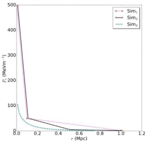
For SIM1and SIM2, we assume an input pressure profile that
matches our nodal model precisely, in order to investigate the ability of our approach to recover the true parameter values in the simplest case. In particular, the pressure profiles for SIM1
and SIM2 are generated by linear interpolation between N = 3
and N = 4 nodes, respectively, and are plotted in Fig. 2. For both simulations, we assume the cluster lies at a redshift of
z=0.5.
For SIM3, we use a more realistic cluster model to test the
abil-ity of our nodal approach to recover a pressure profile that is not of the form assumed in the analysis. In this case, the cluster is simulated using the model described in Olamaie et al. (2012,
2013), which assumes that the dark matter density follows an NFW profile and the ICM plasma pressure is described by the gener-alized NFW (GNFW) profile. The model also assumes that hy-drostatic equilibrium is satisfied and that the local gas fraction is small throughout the cluster. This cluster model is fully spec-ified by just three parameters, for which we assume the values
Mtot(r200)=5×10¹⁴M,z=0.54 andfgas(r200)=0.13. The
re-sulting pressure profile is shown in Fig.2, and is formally singular at
Figure 2. The input pressure profiles for the simulated clusters SIM1, SIM2,
and SIM3. The profiles for SIM1and SIM2were generated by linear
inter-polation betweenN=3 andN=4 nodes, respectively. The profile for SIM3
was generated using the model described in Olamaie et al. (2012,2013), withMtot(r200)=5×10¹⁴M,z=0.54 andfgas(r200)=0.13.
the origin, decreasing sharply with radius in the central regions of the cluster.
5.3 AMI observations of MACS J0744+3927
We also analyze real AMI observations of MACS J0744+3927, one of the clusters in the CLASH (Cluster Lensing And Supernova sur-vey with Hubble) sample (Postman et al.2012). MACS J0744+3927 is a rich cluster at redshiftz=0.689 and has been studied through its X-ray emission, strong lensing, weak lensing, and SZ effect (Schmidt & Allen 2007; Ettori & Balestra2009; Rumsey et al.
2016; Umetsu et al.2016). The SZ signal (decrement) on the AMI map appears circular, (Fig.7in Rumsey et al.2016), in agreement with the X-ray surface brightness from the Chandra archive data (fig.6in Postman et al.2012). Details of AMI-pointed observations towards the cluster, modelling of foreground and background radio point sources and noise, the data reduction pipeline and mapping are described in Rumsey et al. (2016). In particular, we note that the Bayesian analysis includes fitting 23 radio point sources in the AMI field. We focus here, however, on the determination of the parameters defining our nodal model of the cluster.
6 R E S U LT S A N D D I S C U S S I O N
We now present the results of our Bayesian nodal analysis applied to the three simulated data sets SIM1, SIM2, and SIM3, and real
AMI observations of the cluster MACS J0744+3927.
6.1 Simulation SIM1
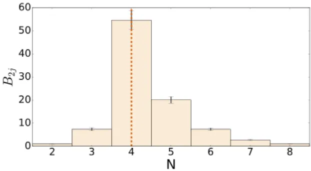
The results of our evidence-based Bayesian model selection analysis to determine the number Nof nodes in the Pe(r) reconstruction
for SIM1are given in Fig.3. This shows the histogram of Bayes
factors B2j, i.e. relative to theN= 2 ‘straight line’ model, as a
function of the number of nodes N in the reconstruction of the pressure profilePe(r) for simulation SIM1. Given our prior choice
πMi =πMjon the models, the Bayes factors are equal to the PORs
P2j, and so the plotted histogram is equivalent to the marginalized
posterior onN. Recalling that the input pressure profile for SIM1
is constructed by linear interpolation between N=3 nodes, one
Figure 3. Histogram of Bayes factorsB2j(i.e. relative to theN=2 model)
as a function of the number of nodesNin the reconstruction of the pressure profilePe(r) for simulation SIM1; this is equivalent to the marginalized
posterior onN. The estimated errors on the Bayes factors are also shown. The vertical dotted line indicates the most-favoured value ofN.
sees that our analysis has recovered the true value ofNas the most-favoured. In particular, it is worth noting that the log Bayes factor lnB23=4.0±0.12, indicating strong evidence for theN=3 model over theN=2 (straight line) model, according to Table1. The Bayes factors then gradually decline forN>3, ultimately reaching the value logB28=0.0±0.12, which indicates no preference forN=
8 over theN=2 model, demonstrating that the ability of theN=
8 model to (over)fit the data is offset by the penalty of its increased complexity.
As mentioned earlier, we will adopt here the straightforward approach of determining the constraints on parameters by condi-tioning on the most-favoured model ˆN=3, rather than performing model averaging according to their Bayes factors. Since it is of interest to understand any biases or constraints on the parameters
imposed by our choice of priors, we first consider the ‘posterior’ Pr(c|D=0,M3) on the cluster parameters obtained in the
ab-sence of any data. This is calculated simply by setting the likeli-hood to a constant value, so that the sampler explores just the prior
π(c). The resulting 1D and 2D marginalized distributions for the
sampling parameterscare shown in Fig.4(left-hand panel); in
addition we plot the derived parameterYtotdefined in equation (7).
These plots show that we correctly recover the assumed prior distri-butions, and also reveal the constraints that our choice of priors has placed on the derived parameterYtot. The plots are produced using
the open source Python librarycorner.py(Foreman–Mackey
2016).
The corresponding plot obtained after analysing the simulation SIM1is shown in Fig.4(right-hand panel), and shows the effect
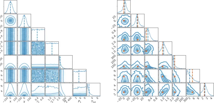
that the data have in updating the prior, via the likelihood func-tion, to produce the posterior, in the spirit of Bayes’ theorem. In particular, one sees that the cluster position (xand y) on the sky is firmly constrained and the true values lie within few arcseconds of the means of the posterior probability distributions forxandy. From the range of posterior distributions in Fig.4, it is clear that the model given the data leads to constraints tighter by a factor of 10. Probability distributions ofxandyfor the no data analysis cover the range−200 and 200, where as the range ofxandyin the analysis including the data is between−20 and 20. Turning to the parameters defining the nodal model of the pressure profile, one sees that the amplitudeP0of the first node is not well constrained,
and we are essentially recovering just the prior distribution. This is to be expected, since an interferometric SZ observation is insensi-tive to length scales on the sky that correspond to Fourier modes in the visibility plane lying well below the shortest baseline (in units of wavelengths) of the interferometer. Consequently, for this
Figure 4. 1D and 2D marginal posterior distributions of the cluster sampling parameterscand the derived parameterYtot, conditioned onN=3 nodes and
obtained in the absence of any data (left) and from analysis of simulation SIM1(right). The horizontal (left to right) and vertical (top to bottom) panels arex
andyin units of arcseconds,r1andr2in Mpc,P0andP1in MeVm−3×10⁻¹, andYtotin Mpc2×10−4, respectively. The contours on the 2D distributions
represent 68 per cent and 95 per cent Bayesian confidence intervals. The vertical dashed blue lines show the mean values of the 1D distributions. The brown squares in the 2-D distributions and the vertical dashed brown lines in the 1D distributions indicate the true values of the parameters used in the simulation. Note that the regions of the parameter space depicted in the right-hand plot are typically much smaller than those in the left-hand one.
Figure 5. The reconstructed pressure profilePe(r) conditioned onN=3
nodes, obtained from analysis of simulation SIM1. Yellow squares show
the positions and amplitudes of the input pressure profile used to generate the simulation. The colour scale shows the relative probability for a recon-structed pressure profilePe(r) to pass through any given pixel in the (r,Pe)
– plane.
simulation, the observations cannot probe the cluster inner core and thus provide no information on the pressureP0at the centre. By
contrast, the position and amplitude of the second node, (r1,P1),
are both constrained relative to their prior distributions, although their 2D marginal reveals a clear degeneracy between them. The positionr2of the third (and final) node is very well constrained.
Since this node corresponds to the point at which the gas pressure drops to zero, it is a valuable quantity for defining the extent of the gas distribution in the cluster. Indeed, obtaining a robust constraint on this quantity can provide insight to the dynamical state of the cluster. Finally, we note that the important derived parameterYtotis
also very well constrained. From their 2-D marginal, however, one sees that there is some degeneracy between the parametersr2and Ytot.
Rather than viewing the posterior constraints on the individual parametersr1,r2,P0,andP1, as in Fig.4, it can be more intuitive
and instructive to plot the corresponding inference on the recon-structed pressure profilePe(r) directly. This may be performed in
a number of ways. For example, one may plot the posterior proba-bility Pr(P|r,D,M3), in normalized slices at constantr(Hee et al.
2016). Here, as shown in Fig.5, we plot simply the relative proba-bility, as determined from the posterior samples, for a reconstructed pressure profilePe(r) to pass through any given pixel in (r,Pe) –
plane. The input pressure profile used to generate the simulation is also plotted (yellow squares). As one might expect from Fig.4
(right-hand panel) and Fig.5, the reconstructed pressure profile is consistent with the input profile, with the true node locations in (r,
Pe)-space all lying within the 68 per cent Bayesian credible
inter-vals of the corresponding inferred node locations. It is again clear, however, that the central pressureP0is poorly constrained, as
dis-cussed above, but that the remaining node parameters are reasonably well determined.
Conditioning onN=3 nodes, we also analyse the SIM1simulated
data assuming a uniform prior onr0between 0 and 0.1 Mpc and plot
the corresponding posterior distributions in Fig.6, which showsr0
is indeed constrained. It should be noted that the constraints on the other parameters remain unchanged.
Figure 6. 1D and 2D posterior distributions ofx,y, andr0, when a uniform
prior between 0 and 0.1 Mpc is placed on the position of first node for SIM1.
xandyare in units of arcseconds, andr0is in Mpc.
Figure 7. As for Fig.3, but for the analysis of simulation SIM2.
In the remainder of the paper, we will plot the reconstructedPe(r),
as in Fig.5, together with the posterior distributions on the position (xandy) of the cluster and the important physical parametersrN−1 ≡rmaxandYtot.
6.2 Simulation SIM2
The histogram of Bayes factorsB2j as a function ofNobtained in
the analysis of simulation SIM2is shown in Fig.7. Recalling that the
input pressure profile for SIM2is constructed by linear interpolation
betweenN=4 nodes, one sees that our analysis has again recovered the true value ofNas the most-favoured. In this case, one sees the
N=2 (straight-line) model is again strongly disfavoured. In partic-ular, one finds lnB24=4.0±0.12, indicating strong evidence for the most-favouredN=4 model over theN=2 model, according to Table1. The Bayes factors then gradually decline forN>4 in a similar way to that found for SIM1, ultimately reaching the value
logB28=0.0±0.12; this again indicates no preference forN=8 over theN=2 model, for the reasons discussed above.
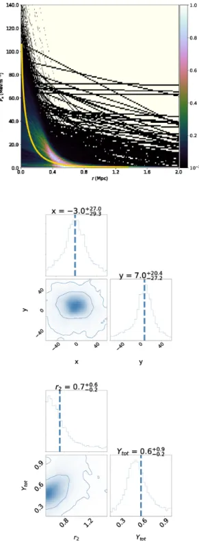
Conditioning onN= 4 nodes, Fig.8shows the reconstructed pressure profile Pe(r) (top panel), and the 1D and 2D marginal
posterior distributions on the cluster position parameters xandy
(middle panel) and on the gas extentr3and total Comptonization
parameterYtot(bottom panel). One again sees that the reconstructed
pressure profile is consistent with the input profile used to generate the simulation, but that cluster gas pressureP0is poorly constrained,
for the reasons we discussed above in the context of SIM1. The
Figure 8. Constraints on cluster parameters, conditioned onN=4 nodes, obtained from analysis of simulation SIM2. Top: the reconstructed pressure
profilePe(r), displayed as in Fig.5, together with the input profile used in
the simulation (yellow squares). Middle: the cluster position parametersx
andy. Bottom: the gas extentr3and total Comptonization parameterYtot.x
andyare in units of arcseconds,rs are in Mpc,Ps are in MeVm−3, andYtotis
in Mpc2×10−4. The contours on the 2D distributions represent 68 per cent
and 95 per cent Bayesian confidence intervals. The vertical dotted lines show the mean values of the 1D distributions; these values and their 68 per cent Bayesian credible intervals are also quoted. The squares and solid vertical lines indicate the true values of the parameters used in the simulation.
Figure 9. As for Fig.3, but for the analysis of simulation SIM3.
remaining node parameters are again reasonably well-constrained, especially the first internal node parameters (r1,P1). Moreover, one
again obtains tight constraints on the cluster position, consistent with the input values. The cluster extentr3and total Comptonization
parameter are also both well-constrained and in agreement with the input values. As in SIM1, however, the 2D marginal distribution of r2andYtotreveals a mild degeneracy.
Further, we analyse the SIM2simulated data conditioning onN=
4 nodes assuming a uniform prior onr0. The results of the analysis
are similar to those found for SIM1and showr0is constrained.
6.3 Simulation SIM3
The histogram of Bayes factorsB2jas a function ofNobtained in
the analysis of simulation SIM3is shown in Fig.9. The input
pres-sure profile for SIM3is not constructed from a linear interpolation
between nodes, but instead from the cluster model of Olamaie et al. (2012,2013), which assumes that the pressure is described by the generalized NFW (GNFW) profile (Nagai et al.2007). Hence, in this case, there is no ‘correct’ number of nodes to recover. Instead, the most-favoured value of ˆN =3 nodes gives an indication of the level of complexity in the pressure profile reconstruction that is sup-ported by the data. Thus, for interferometric SZ observations of the type simulated, the data support only a very simple reconstruction of the pressure profile, favouring a representation consisting of just two straight-line segments. Indeed, the variation of the Bayes factor withNis very similar to that shown in Fig.3for SIM1, for which
the input pressure profile had precisely this simple form.
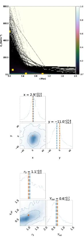
Conditioning onN=3 nodes, Fig.1shows the reconstructed pressure profile Pe(r) (top panel), and the 1D and 2D marginal
posterior distributions on the cluster position parameters xandy
(middle), and the gas extentr3and total Comptonization parameter Ytot(bottom). Although in this simulation there are no ‘correct’
lo-cations for the nodes in (r,Pe)-space, one sees the reconstructedPe
pressure profiles are consistent with the input one. Once again, our analysis serves to highlight the rather coarse level of detail in the re-constructed pressure profile that is achievable with SZ observations of the type simulated. Nonetheless, one still obtains tight constraints on the cluster position, which are consistent with the input values, and also on the cluster extentr3and total Comptonization
parame-ter. We again see, however, that there is a slight degeneracy in the 2D marginal distribution ofr2andYtot.
We also analyse SIM3-simulated data conditioning on N= 3
nodes assuming uniform prior onr0. Once again, we find the results
of the analysis to be similar to those found for SIM1and showr0is
constrained.
Figure 10. As for Fig.8, but conditioned onN=3 nodes, and obtained from the analysis of simulation SIM3.
6.4 Cluster MACS J0744+3927
The histogram of Bayes factorsB2jas a function ofNobtained in the
analysis of real AMI observations of the cluster MACS J0744+3927 is shown in Fig.11. For this real cluster, one sees that the varia-tion of the Bayes factorB2j is broadly similar to that shown in
Fig.9, obtained from the analysis of simulation SIM3, for which
an input GNFW pressure profile was assumed. In particular, the most-favoured model again hasN=3 nodes, after which the Bayes factors gradually decline with increasingN. This indicates that the
Figure 11. As for Fig.3, but for the analysis of real AMI observations of the cluster MACS J0744+3927.
data support a model for the pressure profile that is no more com-plex than two straight-line segments. It is worth noting, however, that in comparing the favouredN=3 model with the baseN=2 (straight-line) model, one obtains lnB23=6.0±0.2, which corre-sponds to a decisive favouring of the former model, according to Table1. Thus, one may deduce at high confidence from our analy-sis, in a model-independent manner, that the pressure profile is not simply a linear function ofr.
Conditioned onN=3 nodes, Fig.10shows the reconstructed pressure profile Pe(r) (top panel), and the 1D and 2D marginal
posterior distributions on the cluster position parameters xandy
(middle), and the gas extentr2and total Comptonization
param-eter Ytot(bottom). Once again, the central pressure P0 is poorly
constrained, but the remaining node locations in (r,Pe)-space are
better determined. It is worth recalling from our analysis of simu-lated data how SZ observations of this type allow for only a very coarse reconstruction of the cluster pressure profile, owing to the SZ effect being proportional to the line-of-sight integral of the pressure. Indeed, from Fig. 10, we recall that in the analysis of simulation SIM3the reconstructed pressure profile was somewhat
flatter than the input GNFW profile, although still consistent with it to within the error-bars, and a similar effect could be occurring in Fig.12.
Nonetheless, as we found in our analysis of simulated data, the cluster position (xandy) is well-constrained, and the corresponding 2-D marginal posterior distribution shows no sign of degeneracy. The gas extentr3and total Comptonization parameterYtotare also
both very well-determined, although their 2-D marginal posterior distribution shows that same slight degeneracy as seen in the anal-yses of the simulation observations.
In the interest of completeness, for this analysis of real AMI observations, we also plot in Fig. 13, the full set of 1D and 2D marginalized posterior distributions for the sampling parameters
c, and the derived parameterYtot.
Since the Bayes factor, plotted in Fig.11suggests that the model, withN=4, 5, and 6 nodes jointly account for similar total probabil-ity as forN=3 model alone, it would be of interest to consider the multi-model inference approach discussed in Section 3, in which the constraints onPe(r) are determined by averaging over all the models MN, weighted by the POR. We postpone this analysis, however, to
a future publication.
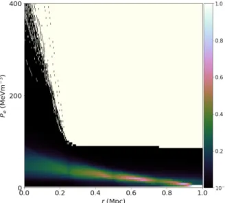
Finally, we compare our reconstructedPe(r) profile in Fig. 12
(top panel) with that obtained using a more mundane approach in which we fix the number and positions of the nodes, which is equivalent to simple radial binning. In particular, we use five equally spaced nodes betweenr=0 andr=1 Mpc (inclusive), where the amplitude of the final node is also fixed. The resulting reconstructed
Figure 12. As for Fig. 10, but conditioned on N = 3 nodes, and obtained from the analysis of real AMI observations of the cluster MACS J0744+3927. Note that the axes are scaled for plotting purposes:
xandyare in units of arcseconds,rs are in Mpc,Ps are in MeVm−3, and
Ytotis in Mpc2×10−4.
Pe(r) profile is shown in Fig.14, in which it should be noted that the
scales on therandPeaxes are somewhat different to those in Fig.12
(top panel). From fig. 14, one sees that the amplitudes of the nodes (each with fixed nodal position) are reasonably well-constrained for
r≥0.4Mpc with almost the same uncertainty for each node in the region. As might be expected, the amplitudes of nodes in the region
r≤0.4Mpc are less well-constrained, with the uncertainty growing significantly as one approachesr=0.
Figure 13. The full set of 1D and 2D marginalized posteriors for the analysis of real AMI observations of the cluster MACS J0744+3927. Note that the axes are scaled for plotting purposes.xandyare in units of arcseconds,rs are in Mpc,Ps are in MeVm−3andYtotis in Mpc2×10−4.
Figure 14. The reconstructed pressure profilePe(r) (conditioned onN=5
nodes and fixed radial bins) obtained from analysis of real AMI observations of the cluster MACS J0744+3927.
Comparing the pressure profile reconstruction with that in Fig.12
(top panel), one sees some interesting differences. In particular, the constraints on the pressure in fig. 12 are much tighter than in Fig.14. Moreover, Fig.12demonstrates far more clearly thervalues over which the data place the strongest constraints on the pressure namely aroundr=0.5 Mpc. Overall, we consider Fig. 12to convey the constraints in the pressure profile more usefully, which illustrates the advantages of our nodal approach.
7 C O N C L U S I O N S
Almost all current approaches to modelling observations of galaxy clusters rely on assuming some parameterized functional form for the properties of the cluster, such as gas density, dark matter density, or temperature. A generic weakness of this approach is that these functional forms have usually been arrived at through empirical means, via the analysis ofN-body simulations or observations, and are often chosen to have simple analytic expressions, rather than being fundamental or physically well motivated.
In this paper, we have moved away from this approach and pre-sented a free-form model for the physical properties of galaxy clus-ters. Previous attempts to model clusters in this way have typically relied simply on dividing the cluster into a predefined number of cells, or concentric shells for spherical clusters, and determining the value of each physical quantity of interest within these subregions (Tchernin et al.2015). Such approaches typically lead to under-determined inverse problems that therefore need to be regularized in some way. There is considerable freedom in how to choose the level or nature of the regularization to apply, and the results can vary significantly depending on how this choice is made. We have therefore presented an alternative approach to free-form reconstruc-tion in which the complexity of the model is determined directly from the data. This is achieved by representing each independent cluster property as some interpolating or approximating function that is specified by a set of control points, or ‘nodes’, for which the number of nodes, together with their positions and amplitudes, are allowed to vary and are inferred from the data in a Bayesian manner, employing both model selection and parameter estimation.
To demonstrate our approach in a simple setting, we have applied it to the particular case of modelling interferometric SZ observa-tions of spherical galaxy clusters. In this context, the free-form part of the cluster model is simply a nodal representation of the elec-tron pressure profilePe(r). We have performed Bayesian analyses
of simulated observations with the Arcminute Microkelvin Imager (AMI) of three separate model clusters.
In the first two simulations, the input pressure profile has the same form as that assumed in the analysis, namely a linear interpolation between a set ofNnodes (withN=3 andN=4, respectively). We showed that, in both cases, our Bayesian model selection analysis returned the true value ofNas the most-favoured. Moreover the resulting reconstructed pressure profiles were consistent with those used as input. In our third simulation, in which the input pressure was assumed to follow a GNFW, the most-favoured model again hadN=3 nodes, and the resulting reconstructed pressure profile was consistent with the input one. In all cases, we found that the central pressure of the cluster is not well-determined, since inter-ferometric observations of the type simulated do not probe length scales corresponding to the inner core. In the analysis of our third simulation, we also noted that the reconstructed pressure profile was somewhat shallower that the singular GNFW profile used to generate the simulation (although still consistent with it), which results from the SZ effect being proportional only to the line-of-sight integral of the pressure in the cluster. A general feature of our results is that SZ interferometric observations of this type allow for only a very coarse reconstruction of the cluster pressure profile. Nonetheless, we also find that in all cases one obtains tight con-straints on the cluster position, and that the cluster extent and total Comptonization parameter are also both well-determined.
We also applied our approach to real AMI observations of the cluster MACS J0744+3927. We found that the most-favoured model has N = 3 nodes. As we found in the analysis of simulations,
the central pressure is poorly determined but the remaining node parameters are reasonably well-constrained. Once again, we found that cluster position, cluster gas extent, and total Comptonization parameter are all very well-constrained.
In closing, some further general points and avenues for future research are worth discussing. First, the tight constraints obtained on the cluster position and on the two very important cluster pa-rametersrmaxandYtotdemonstrate the robustness of our approach.
Moreover, with only minor modification, the method may prove very useful in cluster detection. Although, for the sake of illustra-tion, we assumed the cluster redshift in our analyses presented here, this is not necessary. One can easily re-perform the analysis by instead constructing a nodal model for the pressure profilePe(θ),
whereθ is the projected angle on the sky from the centre of the cluster. In this way, the approach does not depend on the redshift, but will still produce the tight constraints on the cluster position, angular extent, andYtot. It should be pointed out that the detection
algorithm may only be applied in the case where the population of radio point sources is known in advance.
Finally, since our Bayesian approach to the inference produces posterior weighted samples in the parameter space, further direc-tions for future development include defining other derived parame-ters that capture particular features of interest in the pressure profile. One example would be a statistic that embodies the concavity or convexity of the pressure profile. Others might include a parameter that quantifies the cuspy versus core nature of the central region of the cluster. In any case, one may easily use the posterior samples to determine the full (joint) posterior distribution of such derived parameters.
AC K N OW L E D G E M E N T S
The authors thank William Handley for illuminating discussions regarding Bayesian inference. This work was performed using both the Darwin Supercomputer of the University of Cambridge High Performance Computing Service (http://www.hpc.cam.ac.uk/), and COSMOS Shared Memory system at DAMTP, University of Cam-bridge operated on behalf of the STFC DiRAC HPC Facility. Darwin Supercomputer is provided by Dell Inc. using Strategic Research Infrastructure Funding from the Higher Education Funding Council for England and funding from the Science and Technology Facilities Council. COSMOS Shared Memory system is funded by BIS Na-tional E-infrastructure capital grant ST/J005673/1 and STFC grants ST/H008586/1, ST/K00333X/1. We are grateful to Stuart Rankin and COSMOS management team for their computing assistance. MO thanks Astro Hack Week 2016 for valuable discussions and insights on Bayesian inference and statistics. YCP acknowledges support from a Trinity College Junior Research Fellowship.
R E F E R E N C E S
AMI Consortium: Davies et al., 2011,MNRAS, 415, 2708 AMI Consortium: Olamaie M. et al., 2012,MNRAS, 419, 2921 AMI Consortium: Zwart J. T. L. et al., 2008,MNRAS, 391, 1545 Arnaud M., Pratt G. W., Piffaretti R., B¨ohringer H., Croston J. H.,
Pointe-couteau E., 2010, A &A, 517, A92 Bartlett J. G., Silk J., 1994, ApJ, 423, 12 Battaglia N. et al., 2016,JCAP, 8, 013 Birkinshaw M., 1999, PhR, 310, 97
Bonamente M. et al., 2012,NJPh, 14, 025010 Borgani S. et al., 2004,MNRAS, 348, 1078
Carlstrom J. E., Holder G. P., Reese E. D., 2002,ARA &A, 40, 643 Cavaliere A., Fusco-Femiano R., 1976, A&A, 49, 137
Cavaliere A., Fusco-Femiano R., 1978, A&A, 70, 677 Challinor A., Lasenby A., 1998,ApJ, 499, 1 de Haan T. et al., 2016,ApJ, 832, 95
De Martino I., Atrio-Barandela F., 2016,MNRAS, 461, 3222 Ettori S., 2013,MNRAS, 435, 1265
Ettori S., Balestra I., 2009,A&A, 496, 343
Ettori S., Tozzi P., Borgani S., Rosati P., 2004,A&A, 417, 13
Ettori S., Gastaldello F., Leccardi A., Molendi S., Rossetti M., Buote D., Meneghetti M., 2011,A&A, 526, 1
Feroz F., 2013, IEEE 13th International Conference Feroz F., Hobson M. P., 2008,MNRAS, 384, 449
Feroz F., Hobson M. P., Zwart J. T. L., Saunders R. D. E., Grainge K. J. B., 2009,MNRAS, 398, 2049
Feroz F., Hobson M. P., Bridges M., 2009,MNRAS, 398, 1601
Feroz F., Hobson M. P., Cameron E., Pettitt A. N., 2013, preprint (arXiv:1306.2144)
Foreman–Mackey D., 2016, J. Open Source Softw., 24
Giodini S., Lovisari L., Pointecouteau E., Ettori S., Reiprich T. H., Hoekstra H., 2013, SSRv, 177, 247
Grainge K., Jones M. E., Pooley G., Saunders R., Edge A., Grainger W. F., Kneissl R., 2002,MNRAS, 333, 318
Handley W. J., Hobson M. P., Lasenby A. N., 2015,MNRAS, 453, 4384 Hasselfield M. et al., 2013,JCAP, 7, 008
Hee S., Handley W. J., Hobson M. P., Lasenby A. N., 2016,MNRAS, 455, 2461
Hee S., V´azquez J. A., Handley W. J., Hobson M. P., Lasenby A. N., 2017, MNRAS, 466, 369
Hobson M. P., Maisinger K., 2002,MNRAS, 334, 569
Hoekstra H., Bartelmann M., Dahle H., Israel H., Limousin M., Meneghetti M., 2013, SSRv, 177, 75
Itoh N., Kohyama Y., Nozawa S., 1998,ApJ, 502, 7
Jaynes E. T., 1986, Bayesian Methods: an Introductory Tutorial, Cambridge University Press, Cambridge
Jeffreys H., 1961, Theory of Probability, 3rd ed. Oxford: University Press, Oxford
Kass Robert E., Raftery Adrian E., 1995, J. Am. Stat. Assoc., 90, 430 K¨ohlinger F., Hoekstra H., Eriksen M., 2015, MNRAS, 453, 3107 Mantz A. B., Allen S. W., Morris R. G., Rapetti D. A., Applegate D. E.,
Kelly P. L., von der Linden A., Schmidt R. W., 2014,MNRAS, 440, 2077
Munari E., Biviano A., Borgani S., Murante G., Fabjan D., 2013,MNRAS, 430, 2638
Nagai D., Kravtsov A. V., Vikhlinin A., 2007,ApJ, 668, 1 Navarro J. F., Frenk C. S., White S. D. M., 1996,ApJ, 462, 563 Navarro J. F., Frenk C. S., White S. D. M., 1997,ApJ, 490, 493 Nozawa S., Itoh N., Kohyama Y., 1998,ApJ, 508, 17 Olamaie M. et al., 2012,MNRAS, 421, 1136
Olamaie M., Hobson M. P., Grainge K. J. B., 2012,MNRAS, 423, 1534
Olamaie M., Hobson M. P., Grainge K. J. B., 2013,MNRAS, 430, 1344 Olamaie M., Feroz F., Grainge K. J. B., Hobson M. P., Sanders J. S., Saunders
R. D. E., 2015,MNRAS, 446, 1799 Parkinson D., Liddle A. R., 2013, SADM, 6, 3 Perrott Y. C. et al., 2015,A&A, 580, A95 Planck Collaboration et al., 2013,A&A, 550, A128 Planck Collaboration et al., 2016,A&A, 594, A20 Planck Collaboration et al., 2016,A&A, 594, A24 Pointecouteau E., Giard M., Barret D., 1998, A&A, 336, 44 Postman M. et al., 2012,ApJS, 199, 25
Rephaeli Y., 1995, ARA&A, 33, 541
Rines K., Geller M. J., Diaferio A., 2010,ApJ, 715, L180
Rodr´ıguez-Gonz´alvez C., Chary R. R., Muchovej S., Melin J.-B., Feroz F., Olamaie M., Shimwell T., 2017,MNRAS, 464, 2378
Rozo E. et al., 2010,ApJ, 708, 645
Rozo E., Bartlett J. G., Evrard A. E., Rykoff E. S., 2014,MNRAS, 438, 78 Rumsey C. et al., 2016,MNRAS, 460, 569
Saro A., Mohr J. J., Bazin G., Dolag K., 2013,ApJ, 772, 47 Sayers J. et al., 2013,ApJ, 768, 177
Schammel M. P. et al., 2013,MNRAS, 431, 900 Schmidt R. W., Allen S. W., 2007,MNRAS, 379, 209
Seehars S., Amara A., Refregier A., Paranjape A., Akeret J., 2014, PhRvD, 90, 023533
Seehars S., Grandis S., Amara A., Refregier A., 2016, PhRvD, 93, 103507 Sievers J. L. et al., 2013,JCAP, 10, 060
Sif´on C. et al., 2013, ApJ, 772, 25
Sivia D. S., Skilling J., 2005, Data Analysis: a Bayesian Tutorial. Oxford University Press, Oxford
Sunyaev R. A., Zeldovicationh Y. B., 1970, CoASP, 2, 66
Tchernin C., Majer C. L., Meyer S., Sarli E., Eckert D., Bartelmann M., 2015,A&A, 574, A122
Trotta R., Feroz F., Hobson M., Roszkowski L., Ruiz de Austri R., 2008, JHEP, 12, 024
Umetsu K., Zitrin A., Gruen D., Merten J., Donahue M., Postman M., 2016, ApJ, 821, 116
V´azquez J. A., Bridges M., Hobson M. P., Lasenby A. N., 2012,JCAP, 6, 006
V´azquez J. A., Bridges M., Hobson M. P., Lasenby A. N., 2012,JCAP, 9, 020
Vikhlinin A. et al., 2009,ApJ, 692, 1060
Vikhlinin A., Markevitch M., Murray S. S., Jones C., Forman W., Van Speybroeck L., 2005,ApJ, 628, 655
Vikhlinin A., Kravtsov A., Forman W., Jones C., Markevitch M., Murray S. S., Van Speybroeck L., 2006,ApJ, 640, 691
This paper has been typeset from a TEX/LATEX file prepared by the author.