W O R K I N G PA P E R S E R I E S
N O. 3 7 7 / J U LY 2 0 0 4
OPTIMAL MONETARY
POLICY UNDER
COMMITMENT WITH
A ZERO BOUND ON
NOMINAL INTEREST
RATES
In 2004 all publications will carry a motif taken from the €100 banknote.
W O R K I N G PA P E R S E R I E S
N O. 3 7 7 / J U LY 2 0 0 4
OPTIMAL MONETARY
POLICY UNDER
COMMITMENT WITH
A ZERO BOUND ON
NOMINAL INTEREST
RATES
1by Klaus Adam
2and Roberto M. Billi
3This paper can be downloaded without charge from http://www.ecb.int or from the Social Science Research Network electronic library at http://ssrn.com/abstract_id=557703.
© European Central Bank, 2004 Address
Kaiserstrasse 29
60311 Frankfurt am Main, Germany
Postal address Postfach 16 03 19
60066 Frankfurt am Main, Germany
Telephone +49 69 1344 0 Internet http://www.ecb.int Fax +49 69 1344 6000 Telex 411 144 ecb d
All rights reserved.
Reproduction for educational and non-commercial purposes is permitted provided that the source is acknowledged.
The views expressed in this paper do not necessarily reflect those of the European
C O N T E N T S
Abstract 4
1 Non-technical summary 5
2 Introduction 7
3 Related literature 11
4 The monetary policy problem 12
4.1 Discussion 14
4.1.1 Relation to earlier work 14
4.1.2 Policy instruments 14
4.1.3 How much non-linearity? 15
5 Model calibration 17
7 Optimal policy with lower bound 20
7.1 Optimal policy functions 20
7.2 Dynamic response to real rate shocks 23
7.3 Frequency of binding rates and welfare
implications 24
7.4 Global implications of binding shocks 25
8 Sensitivity analysis 26
8.1 More variable shocks 27
8.2 Lower interest rate elasticity of output 28
9 Conclusions 29
A Appendix 30
A.1 Identification of historical shocks
(baseline calibration) 30
A.2 Numerical algorithm 33
A.3 Identification of historical shocks
(RBC calibration) 35
References 36
51
Tables and figures
European Central Bank working paper series
40
Abstract
We determine optimal monetary policy under commitment in a forward-looking New Keynesian model when nominal interest rates are bounded be-low by zero. The be-lower bound represents an occasionally binding constraint that causes the model and optimal policy to be nonlinear. A calibration to the U.S. economy suggests that policy should reduce nominal interest rates more aggressively than suggested by a model without lower bound. Rational agents anticipate the possibility of reaching the lower bound in the future and this amplifies the effects of adverse shocks well before the bound is reached. While the empirical magnitude of U.S. mark-up shocks seems too small to entail zero nominal interest rates, shocks affecting the natural real interest rate plausibly lead to a binding lower bound. Under optimal policy, however, this occurs quite infrequently and does not require targeting a positive average rate of inflation.
ment, liquidity trap, New Keynesian
Keywords: nonlinear optimal p olicy, zero i nterest rate b ound,
1
In the recent past nominal interest rates in major world economies have reached historically low levels. The inability to further lower nominal inter-est rates can lead to higher than desired real interinter-est rates and it is often feared that the economy might then embark on a deflationary path, often referred to as a ‘liquidity trap’.
Using a standard monetary policy model with nominal rigidities, the so-called New Keynesian model, and taking explicitly into account that nominal interest rates cannot be set to negative values, this paper determines the quantitative implications of the zero lower bound for the U.S. economy using estimates of the shock processes that hit the economy during the period 1983-2002.
The zero lower bound on nominal interest rates constrains monetary pol-icy because adverse shocks might create a situation where ideally the polpol-icy- policy-maker would set negative nominal interest rates. We ask for the importance of this contraint in the U.S. economy and clarify how monetary policy should be conducted in a situation where interest rates are only slightly positive and there is the possibility of reaching the lower bound in the future. The latter appears especially relevant in the current era of low inflation and low nominal interest rates.
When there is the possibility that future shocks push the economy into a situation with zero nominal interest rates, it is optimal to lower nominal rates more aggressively in advance, i.e., already before hitting the bound. Such ‘preemptive’ action is optimal because agents anticipate the possibility of binding shocks in the future and thereby tend to amplify the effects of adverse shocks. A stronger policy response counteracts this amplification.
cause the lower bound to become binding in the U.S. economy, but this happens relatively infrequently and is a feature of optimal policy. Based on our estimates for the 1983-2002 period, the bound can be expected to bind under optimal policy in one quarter every 17 years on average.
Once zero nominal interest rates are reached, policy should promise to increase nominal interest rates in the future less strongly and to allow mod-erate amounts of inflation. Provided the promise is credible, this genmod-erates inflationary expectations and effectively lowers the real interest rates that agents are confronted with.
We also consider whether there is any need to have a positive target rate for inflation in order to buffer against the risk of hitting the zero lower bound on nominal interest rates. For a range of model parameterizations wefind such a buffer to be suboptimal.
Besides addressing substantive economic questions, this paper also im-plements a new approach to numerically solving nonlinear optimal policy problems with forward-looking constraints that might be of wider interest.
2
Introduction
In the recent past nominal interest rates in major world economies have reached historically low levels and in some cases have gone all the way down to zero.1 Such a situation is generally deemed problematic as the inabil-ity to further lower nominal interest rates can lead to higher than desired real interest rates. In particular, it is often feared that if agents hold de-flationary expectations the economy might embark on a dede-flationary path, often referred to as a ‘liquidity trap’, with high real interest rates generating demand shortfalls and thereby fulfilling the expectations of falling prices.
This paper studies optimal monetary policy under commitment taking explicitly into account that nominal interest rates cannot be set to negative values.2 We consider a well-known monetary policy model with monopolistic competition and sticky prices, as described in Clarida, Galí and Gertler (1999) and Woodford (2003). While this model has been widely used to study optimal monetary policy and short-run fluctuations, we are thefirst to solve it in a fully stochastic setup that directly takes into account the zero lower bound.
In a stochastic economy the lower bound on interest rates will occa-sionally be binding, since shocks may drive the economy into a situation where it would be better for monetary policy to set nominal rates below zero. This feature aggravates the solution of the policy problem but allows us to calibrate the model to the U.S. economy and to assess the quantitative
1At April 30, 2004 the U.S. federal funds rate stood at 1%, the uncollateralized
overnight call rate in Japan was at 0,001%, and the minimum bid rate of the European Central Bank was at 2%.
2
In principle negative nominal rates are feasible, e.g., if one is willing to give up free
convertability of deposits and otherfinancial assets into cash or if one could levy a tax on
money holdings, see Buiter and Panigirtzoglou (2003) and Goodfriend (2000). However, there seems to be no general consensus on the applicability of such policy measures.
implications of the zero lower bound. In particular, we can ask how optimal monetary policy should be conducted when interest rates are only slightly positive and there is the possibility of reaching the lower bound in the fu-ture. This is especially relevant in the current era of low inflation and low nominal interest rates, that characterize major world economies.
Besides addressing substantive economic questions, this paper also im-plements a new approach to numerically solving nonlinear optimal policy problems with forward-looking constraints that might be of wider inter-est. In particular, we use results from the theory of recursive contracts, see Marcet and Marimon (1998), and determine optimal policy by solving for the functionalfixed point of a generalized Bellman equation.3 This solution method is complementary to the approach of Marcet and DenHaan (1990) and Christiano and Fisher (2000), which is based on solving a system of first order conditions, but it has the paramount advantage that one can numerically verify whether second order conditions actually hold.
Two qualitatively new features of optimal policy emerge from our anal-ysis.
First, wefind that nominal interest rates may have to be lowered more aggressively in response to shocks than what is instead suggested by a model without lower bound. Such ‘preemptive’ easing of nominal rates is optimal because agents anticipate the possibility of binding shocks in the future and reduce already today their output and inflation expectations correspond-ingly.4 Such expectations end up amplifying the adverse effects of shocks and thereby trigger a stronger policy response.
3To our knowledge we are thefirst to solve for the saddle point function solving the
generalized Bellman equation. 4
Expectations are reduced because once the lower bound is reached inflation and output
Second, the presence of shocks that cause the zero lower bound to bind alters also the optimal policy reaction to non-binding shocks. This occurs because the policymaker cannot affect the average real interest rate in any stationary equilibrium, therefore, faces a ‘global’ policy constraint. The inability to lower nominal and real interest rates as much as desired requires that optimal policy increases rates less (or lowers rates more) in response to non-binding shocks, compared to the policy that would instead be optimal in the absence of the lower bound.
There are also a number ofquantitative results regarding optimal mon-etary policy for the U.S. economy emerging from this analysis.
First, the zero lower bound appears inessential in dealing with mark-up shocks, i.e., variations over time in the degree of monopolistic competition betweenfirms.5 More precisely, the empirical magnitude of mark-up shocks observable in the U.S. economy for the period 1983-2002 is too small for the zero-lower bound to become binding. This would remain the case even if the true variance of mark-up shocks were threefold above our estimated value.
Second, the shocks to the ‘natural’ real rate of interest may cause the lower bound to become binding, but this happens relatively infrequently and is a feature of optimal policy.6 Based on our estimates for the 1983-2002 period, in the U.S. economy the bound would be expected to bind on average one quarter every 17 years under optimal policy.7 Once zero nominal interest rates are observed they are expected to endure on average not more than 1 to 2 quarters. Moreover, the average welfare losses entailed by the zero lower bound seem to be rather small.
5These shocks are sometimes called ‘cost-push’ shocks, e.g., Clarida et al. (1999).
6
The natural real rate is the real interest rate associated with the optimal use of
productive resources underflexible prices.
The latter results, however, are sensitive to the size of the standard deviation of the estimated natural real rate process. In particular, wefind that zero nominal rates would occur much more frequently and generate higher welfare losses if the real rate process had a somewhat larger variance. Third, as argued by Jung, Teranishi, and Watanabe (2001) and Eggerts-son and Woodford (2003) optimal policy reacts to a binding zero lower bound on nominal interest rates by generating inflationary expectations in the form of a commitment to let future output gaps and inflation rates increase above zero. The policymaker thereby effectively lowers the real interest rates that agents are confronted with.
Since reducing real rates using inflation is costly (in welfare terms), the policymaker has to trade-off the welfare losses generated by too high real rates with those stemming from higher inflation rates. We find that the required levels of inflation and the associated positive output gap are very moderate. A negative 3 standard deviation shock to the natural real rate requires a promise of an increase in the annual inflation rate in the order of 15 basis points and a positive output gap of roughly 0.5%.
Finally, while the optimal policy response to shocks through the promise of above average output and inflation may in principal generate a ‘commit-ment bias’, the quantitative effects turn out to be negligible. This holds not only for our baseline calibration but also for a range of alternative model parameterizations that we look at. It suggests that optimal policy for the U.S. economy implements an average inflation rate of zero even when taking directly into account the zero lower bound on nominal interest rates.8
8
Zero inflation is optimal because it minimizes the price dispersion betweenfirms with
sticky prices and we abstract from the money demand distortions associated with positive nominal interest rates.
discusses the related literature. Thereafter, section 4 introduces the model and the policy problem. Section 5 presents our calibration for the U.S. economy. The solution method we employ is described in section 6. Section 7 presents our main results on the optimal monetary policy with lower bound for the U.S. economy. We then discuss in section 8 the robustness of our findings to various parameter changes, and briefly conclude in section 9.
3
A number of recent papers study the implications of the zero lower bound on nominal interest rates for optimal monetary policy.
Most closely related is Eggertsson and Woodford (2003) who consider a perfect foresight economy and analytically derive optimal targeting rules with a lower bound. In this paper we consider instead a fully stochastic setup which requires to solve the model numerically. Only with this stochastic setup one can assess how policy should be conducted in the ‘run-up’ to a binding situation, where shocks may drive the economy from a non-binding state into a binding one. In addition, we can calibrate the model to the U.S. economy and study the quantitative importance of the zero lower bound for the conduct of monetary policy in practice.
A related set of papers focuses on optimal monetary policy in the ab-sence of credibility. In a companion paper of ours, Adam and Billi (2003), we derive the nonlinear optimal policy under discretionary policy making. Eggertsson (2003) analyzes discretionary policy and the role of nominal debt policy as an instrument to achieve credibility.
The performance of simple monetary policy rules is examined by Fuhrer and Madigan (1997), Wolman (2003), and Coenen, Orphanides and Wieland (2004). A main finding of this set of papers is that if the targeted infla-The remainder of this paper is structured as follows. Section 3 briefly
tion rate is close enough to zero, simple policy rules formulated in terms of inflation rates, e.g., the Taylor rule (1993), can generate significant real distortions. Reifschneider and Williams (2000) and Wolman (2003) show that simple policy rules formulated in terms of a price level target can sig-nificantly reduce these real distortions associated with the zero lower bound Benhabib et al. (2002) study the global properties of Taylor-type rules showing that these might lead to self-fulfilling deflation that converges to a low inflation or deflationary steady state. Evans and Honkapohja (2003) study the properties of global Taylor rules under adap-tive learning, showing the existence of an additional steady state with even lower inflation rates.
The role of the exchange rate and monetary-base rules in overcoming the adverse effects of a binding lower bound on interest rates is analyzed, e.g., by Auerbach and Obstfeld (2003), Coenen and Wieland (2003), McCallum (2003), and Svensson (2003).9
4
We consider a simple and well-known monetary policy model of a represen-tative consumer and firms in monopolistic competition facing restrictions on the frequency of price adjustments (Calvo (1983)). Following Rotemberg (1987), this is often referred to as the ‘New Keynesian’ model, that has fre-quently been studied in the literature, e.g., Clarida, Galí and Gertler (1999) and Woodford (2003).
We augment this otherwise standard monetary policy model by explicitly imposing the zero lower bound on nominal interest rates. We thus consider
9
Further articles dealing with the relevance of the zero lower bound can be found in the special issues of the Journal of Japanese and International Economies Vol. 14, 2000 and the Journal of Money Credit and Banking Vol. 32 (4,2), 2000.
on interest rates.
the following problem: max {yt,πt,it} −E0 ∞ X t=0 βt¡πt2+αyt2¢ (1) s.t.: πt=βEtπt+1+λyt+ut (2) yt=Etyt+1−ϕ(it−Etπt+1) +gt (3) it≥ −r∗ (4) ut=ρuut−1+εu,t (5) gt=ρggt−1+εg,t (6) u0,g0 given (7)
where πt denotes the inflation rate, yt the output gap, and it the nominal
interest rate expressed as deviation from the interest rate consistent with the zero inflation steady state.
The monetary policy objective (1) is a quadratic approximation to the utility of the representative household, where the weight α > 0 depends on the underlying preference and technology parameters. Equation (2) is a forward-looking Phillips curve summarizing, up to first order, profit-maximizing price setting behavior by firms, where β ∈ (0,1) denotes the discount factor andλ>0depends on the underlying utility and technology parameters. Equation (3) is a linearized Euler equation summarizing house-holds’ intertemporal maximization, where ϕ > 0 denotes the interest rate elasticity of output. The shockgtcaptures the variation in the ‘natural’ real
interest rate and is usually referred to as a real rate shock, i.e.,
gt=ϕ(rt−r∗) (8)
where the natural real rate rt is the real interest rate consistent with the
zero inflation steady state.10 The requirement that nominal interest rates have to remain positive is captured by constraint (4). Finally, Equations (5) and (6) describe the evolution of the shocks, where ρj ∈ (−1,1) and
εj,t ∼iiN(0,σ2j) forj=u, g.11
4.1
Discussion
4.1.1 Relation to earlier work
The new feature of our policy problem, outlined in the previous section, is the presence of the lower bound (4) and the shocksεu,tand εg,t. These
ele-ments together cause the policy problem to become nonlinear. The problem without lower bound has been studied, e.g., by Clarida, Galí and Gertler (1999) and Woodford (2003). The problem with lower bound and perfect foresight (εu,t=εg,t= 0) has been analyzed in Jung, Teranishi, and
Watan-abe (2001) and Eggertsson and Woodford (2003).12
4.1.2 Policy instruments
It should be stressed that the interest rate is here assumed to be the only available policy instrument. We thereby abstract from a number of alter-native policy instruments that might be important in a situation of zero nominal interest rates, most notablyfiscal policy, exchange rate policy, and quantity-based monetary policies. Our setup, thus, tends to give prominence if not overemphasize the policy implications of the zero nominal interest rate
1 0The shockg
t summarizes all shocks that underflexible prices generate time variation
in the real interest rate, therefore, it captures the combined effects of preference shocks,
productivity shocks, and exogenous changes in government expenditure. 1 1
As shown subsequently, this specification of the shock processes is sufficiently general
to describe the historical sequence of shocks in the U.S. economy for the period 1983:1-2002:4 that we consider.
1 2
Eggertsson and Woodford (2003) also consider a simple stochastic setup with an ab-sorbing non-binding state.
While the omission of fiscal policies clearly constitutes a shortcoming that ought to be addressed in future work, ignoring exchange rate and money policies may be less severe than one might initially think.
Clarida, Galí and Gertler (2001), e.g., show that one can reinterpret the present setup as an open economy model and that there exists a one-to-one mapping between interest rate policies and exchange rate policies. It is then inessential whether policy is formulated in terms of interest rates or exchange rates.
Similarly, ignoring quantity-oriented monetary policies in the form of open market operations during periods of zero nominal interest rates seems to be of little relevance. Eggertsson and Woodford (2003) show that in the present model such policies have no effect on the equilibrium unless they influence the future path of interest rates.
We recognize that alternative policy instruments may still be relevant in practice.13 Focusing on interest rate policy in isolation is nevertheless of interest, since it allows to assess what interest rate policy alone can achieve in avoiding liquidity traps and whether there is any need for employing other instruments. This seems important to know, given that alternative instruments are often subject to (potentially uncertain) political approval by external authorities and may therefore not be readily available.
4.1.3 How much non-linearity?
Instead of the fully nonlinear model, we study linear approximations to firms’ and households’ first order conditions, i.e., equations (2) and (3),
1 3See Eggertsson (2003) on how other policy instruments, e.g., nominal debt policy, may
respectively, and a quadratic approximation to the objective function, i.e., equation (1). This means that the only nonlinearity that we take account of is the one imposed by the zero lower bound (4).14
Clearly, this modelling approach has advantages and disadvantages. One disadvantage is that for the empirically relevant shock support and the esti-mated value of the discount factor the linearizations (2) and (3) may perform poorly at the lower bound. Yet, this depends on the degree of nonlinearity present in the economy, an issue about which relatively little is empirically known.
A paramount advantage of our approach is that one can economize in the dimension of the state space. A fully nonlinear setup would require an additional state to keep track over time of the higher-order effects of price dispersion, as shown by Schmitt-Grohé and Uribe (2003). Computational costs would become prohibitive with such an additional state.15
A further advantage of focusing solely on the nonlinearities induced by the lower bound is that one does not have to parameterize higher order terms when calibrating the model. This seem important, given the lack of empirical evidence on this matter.
Finally, the simpler setup implies that our results remain more easily comparable to the standard linear-quadratic analysis without lower bound that appears in the literature, as the only difference consists of imposing equation (4).
1 4Technically, this approach is equivalent to linearizing thefirst order conditions of the
nonlinear Ramsey problem around thefirst best steady state except for the non-negativity
constraint for nominal interest rates, that is kept in its original nonlinear form. This is
true because derivingfirst order conditions and linearizing thereafter is equivalent tofirst
linearizing and then taking derivatives. 1 5
Our model has 4 state variables with continuous support and it takes already 39 hours to obtain convergence on a Pentium 4 with 2.6 GHz.
5
To assess the quantitative importance of the zero lower bound for monetary policy, we assign parameter values for the coefficients appearing in equations (1) to (6) by calibrating the model to the U.S. economy.
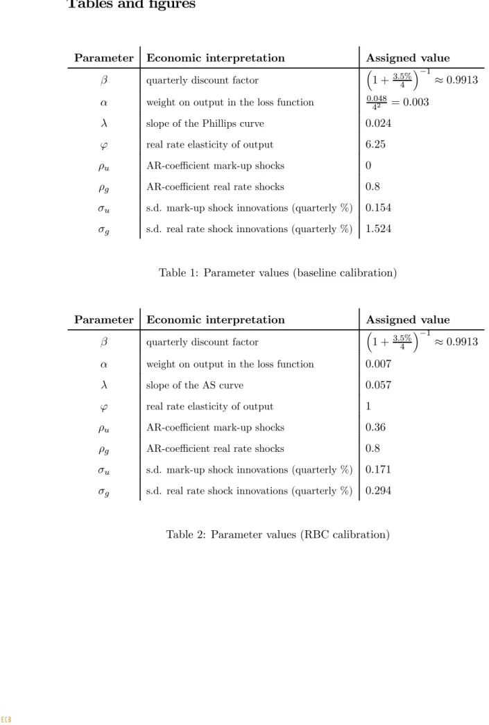
Table 1 summarizes our baseline parameterization. The values forα,λ, and ϕare taken from table 6.1 in Woodford (2003). The parameters of the shock processes and the discount factor are estimated using U.S. data for the period 1983:1-2002:4, following the approach of Rotemberg and Woodford (1998). Details of the estimation and reasons for the sample period chosen are given in appendix A.1.
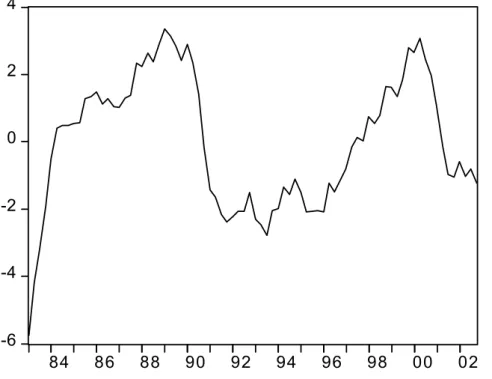
The identified historical shock series are shown in figure 3. Mark-up shocks do not display any significant autocorrelation and have a standard deviation of approximately0.61%annually.16 Real rate shocks, however, are
rather persistent. As one would expect, the natural real rate seems to fall during recessions, e.g., at the beginning of the 1990s and at the start of the new millennium. The implied annual standard deviation of the natural real rate, as implicitly defined in equation (8), is equal to1.63%annually.17
The robustness of our findings to various assumptions regarding the pa-rameterization of the model is considered in section 8.
1 6
This lack of autocorrelation contrasts with Ireland (2002) who uses data starting in 1948:1. Extending our sample back to this date would also lead to highly persistent
mark-up shocks. But our identification of shocks requires the absence of structural breaks, so
we restrict attention to the shorter sample period. 1 7
When using instead the period 1979:4-1995:2 as in Rotemberg and Woodford (1998),
which includes the volatile years 1980-1982, wefind an annual standard deviation of 2.57%
for the natural real rate.
Due to the presence of an occasionally binding constraint in the model, analytical results for optimal policy are unavailable. For this reason we have to rely on numerical methods.
An important complication that arises is that the policymaker’s maxi-mization problem fails to be recursive, since constraints (2) and (3) involve forward-looking variables. For this reason we cannot directly resort to dy-namic programming techniques; these assume transition equations that do not involve expectation terms. To obtain a dynamic programming formula-tion we apply the technique of Marcet and Marimon (1998) and reformulate the policy problem (1)-(7) as follows:
W(µ1t, µ2t, ut, gt) = inf (γ1 t,γt2) sup (yt,πt,it) © h(yt,πt, it,γt1,γt2, µ1t, µ2t, ut, gt) +βEtW(µ1t+1, µ2t+1, ut+1, gt+1) ª (9) s.t.: it≥ −r∗ µ1t+1=γt1 µ2t+1=γt2 ut+1 =ρuut+εu,t+1 gt+1=ρggt+εg,t+1 µ10 = 0 µ20 = 0 u0, g0 given where h¡y,π, i,γ1,γ2, µ1, µ2, u, g¢ ≡ −αy2−π2+γ1(π−λy−u)−µ1π +γ2(y+ϕi−g)−µ2 1 β(ϕπ+y). (10)
Equation (9) is a generalized Bellman equation, requiring maximization with respect to the controls (yt,πt, it) and minimization with respect to the
La-grange multipliers¡γ1 t,γt2
¢
. Marcet and Marimon (1998) call expressions as equation (9) a recursive saddle point functional equation.
One should note that the reformulated problem (9) is fully recursive, since the transition equations now involve only lagged state variables. This problem has, however, two additional state variables (µ1, µ2), bringing the total number of state variables up to four. The states(µ1, µ2)are the lagged values of the Lagrange multipliers for the constraints (2) and (3), respec-tively; they can be interpreted as ‘promises’ that have to be kept from past commitments. A negative value ofµ1, e.g., indicates a promise to generate higher inflation rates than what purely forward looking policy would im-ply. This follows from the expression of the one-period return functionh(·) given in equation (10). Likewise, a negative value ofµ2 indicates a promise to generate values of 1β(ϕπ+y) higher than what purely forward looking policy suggests.
Instead of deriving the first order conditions of problem (9) and trying to solve the resulting system of equations, which is the standard approach in the literature, e.g., Christiano and Fisher (2000), we approximate the value function that solves the recursive saddle point functional equation (9). It appears that we are thefirst to actually solve for the saddle point function of such a recursive problem and doing so has two important advantages.
First, the value function approach allows us to verify whether second order conditions hold. In particular, we numerically check if the right-hand side of (9) is a saddlepoint, i.e., a minimum with respect to (γ1
t,γt2) and a
maximum with respect to (yt,πt, it), respectively, at the conjectured
opti-mal policy.18 As is well known, e.g., chapter 14.3 in Silberberg (1990), the
saddle point property is a sufficient condition for having found a constrained optimum.
Second, results in Marcet and Marimon (1998) show that, given certain conditions, the mapping defined by equation (9) is a contraction as for a standard dynamic programming problem. Therefore, standard value func-tion iterafunc-tion methods deliver convergence to the fixed point. Indeed, to solve for the fixed point we iterate on this generalized Bellman equation until convergence is achieved. The numerical algorithm used is described in appendix A.2.
The next sections present the results obtained with our solution ap-proach.
7
This section describes the optimal policy with a lower bound on nominal interest rates for the calibration to the U.S. economy shown in table 1. All variables are expressed as percentage deviations from steady state; both inflation rates and interest rates are transformed into annual rates.
7.1
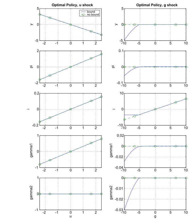
Figure 4 presents the optimal responses of (y,π, i) and the Lagrange mul-tipliers (γ1,γ2) to both a mark-up shock and a real rate shock.19 The responses of the Lagrange multipliers are of interest because they represent
simultaneous deviations from the conjectured optimum for(γ1
t,γt2)and(yt,πt, it),
respec-tively, at a large number of points in the state space. Due to the recursive structure of the
problem it thereby suffices to verify the saddle point property for one-period deviations
only.
1 9The state variables not shown on thex-axes are set to their (unconditional) average
values. Policies are shown for a range of ±4unconditional standard deviations of both
the mark-up shock and the real rate shock.
Optimal policy with lower bound
commitments regarding future inflation rates and output levels, as explained in the previous section. Depicted are the optimal policy responses both for the case of the zero lower bound being imposed (solid line) and for the case of interest rates allowed to become negative (dashed line with circles).
The left-hand panel offigure 4 shows that the optimal response to mark-up shocks is virtually unaffected by the presence of the zero lower bound.20 Independently of whether the bound is imposed or not, a positive mark-up shock lowers output and leads to a promise of future deflation, as indicated by the positive value of γ1. The latter ameliorates the inflationary effect of the shocks through the expectational channel present in equation (2). To deliver on its promise the policymaker increases nominal interest rates.21 Yet, the required interest rate changes are rather small, implying that mark-up shocks do not plausibly lead to a binding lower bound.
The situation is quite different if we consider the policy response to a real rate shock, as depicted on the right-hand panel of figure 4. Without zero lower bound these shocks do not generate any policy trade-off: the re-quired real rate can be implemented through appropriate variations in the nominal rate alone. Once the lower bound is imposed, sufficiently negative real rate shocks cause the bound to be binding, so promising future inflation remains the only instrument for implementing reductions in the real rate. The negative values ofγ1 andγ2reveal that once the lower bound is reached the policymaker indeed commits to future inflation as a substitute for nom-inal rate cuts. Yet, inflation is a costly instrument (in welfare terms) and
2 0
The optimal reaction to mark-up shocks is different with or without the bound, but
the difference is quantiatively small for the calibrated parameter values. We will come
back to this point in section 7.4. 2 1
The sign of the optimal interest rate response, however, depends on the degree of autocorrelation of the mark-up shocks. In particular, with more persistent shocks nominal rates would optimally decrease in response to a positive mark-up shock.
it would be suboptimal to completely undo the output losses generated by negative real rate shocks. As a result, there is a negative output gap, some deflation, and nominal interest rates are at their lower bound. All these features are generally associated with a ‘liquidity trap’.
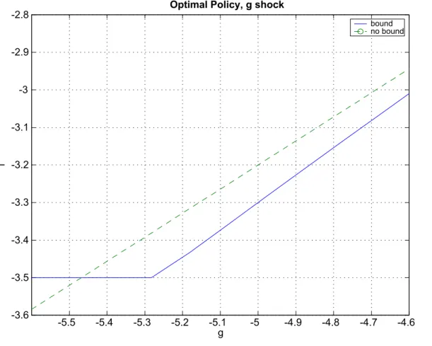
Figure 5 depicts the optimal interest rate response to real rate shocks in greater detail. This reveals that it is optimal to reduce nominal rates more aggressively than is the case when nominal rates are allowed to become negative. Therefore, the lower bound is reached earlier.22 A stronger interest rate reduction is optimal because the possibility of a binding lower bound in the future places downward pressure on expected future output and inflation, since these variables become negative once the bound is reached, see the right-hand panel offigure 4. The reduced output and inflation expectations amplify the effects of negative real rate shocks in equation (3), thereby require that the policymaker lowers nominal rates faster.
This amplification effect via private sector expectations points towards an interesting complementarity between policy decisions and private sector expectations formation that may be of considerable importance for actual policy making. Suppose, e.g., that agents suddenly assign a larger probabil-ity to the lower bound being binding in the future. Since this lowers output and inflation expectations, policy would reduce the nominal interest rate and cause the economy to move into the direction of the expected change. The existence of possible sunspotfluctuations, however, is an issue that has to be explored in future work.
2 2
Kato and Nishiyama (2003) found a similar effect with a backward looking AS curve,
which suggests that our result is robust to the introduction of lagged inflation terms into
the ‘New Keynesian’ AS curve. Using different models, Orphanides and Wieland (2000)
and Reifschneider and Williams (2000) also report more aggressive easing than in the absence of the zero bound.
7.2
Figure 6 displays the mean response of the economy to real rate shocks of
±3 unconditional standard deviations.23 With our baseline calibration of table 1 the annual ‘natural’ real rate, i.e., the real interest rate consistent with the efficient use of productive resources, stands temporarily at+8.39% and −1.39%, respectively; the interesting case being the one where full use of productive resources requires a negative real rate.
As argued by Krugman (1998), negative real rates are plausible even if the marginal product of physical capital remains positive. For instance agents may require a large equity premium, e.g., historically observed in the U.S., or the price of physical capital may be expected to decrease.
Figure 6 shows that in response to a negative real rate shock annual infla-tion rises by about 15 basis points for up to 3 or 4 quarters and then returns to a value close to zero. Similarly, output increases slightly above potential from the second quarter and slowly returns to potential. Getting out of a ‘liquidity trap’ induced by negative real-rate shocks, therefore, requires that the policymaker promises to let future output and inflation increase above zero for a substantial amount of time. The qualitative feature of thisfinding is already reported in Eggertsson and Woodford (2003), and in a somewhat different way in Auerbach and Obstfeld (2003). Our results tend to clarify, however, that the required amount of inflation and the output boom are rather modest.
2 3
Since in this nonlinear model certainty equivalence fails, instead of the more familiar deterministic impulse responses we discuss results in terms of the implied ‘mean dynamics’ in response to shocks. The mean dynamics in this and other graphs are the average responses computed for 100 thousand stochastic simulations. The initial values for the
other states are set equal to their unconditional average values. Setting them to the
conditional average values consistent with the real rate shock does not make a noticable
difference.
One should note that ex-post there would be strong incentives to increase nominal interest rates earlier than promised, since this would bring both inflation and output closer to their target values. The feasibility of the optimal policy response, therefore, crucially depends on the policymaker’s credibility. Wether policymakers can and may want to credibly commit to such policies is currently subject of debate, e.g.,Orphanides (2003).24
7.3
In this section we discuss the frequency with which the zero lower bound can be expected to bind and welfare implications.
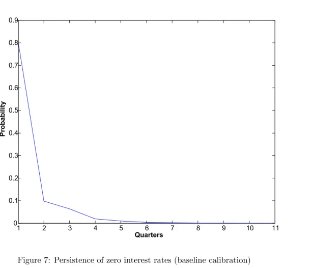
Under optimal policy for the calibration to the U.S. economy the lower bound binds rather infrequently, namely in about one quarter every 17 years on average. Moreover, zero nominal interest rates tend to prevail for rather short periods of time (roughly 1.4 quarters on average). Figure 7 displays the probability with which the zero bound is binding fornquarters, conditional on it being binding in quarter one. The likelihood that zero nominal interest rates persist for more than 4 quarters is merely 1.8%.
Since the lower bound is hit rather infrequently, possible biases for av-erage output and inflation emerging from the nonlinear policy functions are expected to be small. In fact, our simulations show that for the calibration at hand there are virtually no average level effects for these variables.25
Finally, as one would expect, the average welfare effects generated by the existence of a zero lower bound are rather small. Our simulations show that the additional welfare losses of the zero lower bound are roughly 1% of those
2 4Interestingly, the Bank of Japan has recently announced explicit macroeconomic
con-ditions that have to be fulfilled before it may consider abandoning its current zero interest
rate policy.
2 5Average output and inflation deviate less than 0.01% from their steady state values.
generated by the stickiness of prices alone.26 Since the zero lower bound is reached rather infrequently, the conditional welfare losses associated with being at the lower bound can nevertheless be quite substantial.
7.4
This section reports a qualitatively newfinding that stems from the presence of binding negative real rate shocks. It turns out that binding shocks alter the optimal policy response to non-binding shocks, i.e., positive real rate shocks and mark-up shocks of both signs. In this sense, the existence of a lower bound has global implications on the shape of the optimal policy functions.
For the baseline parameterization of the U.S. economy given in table 1, however, these global effects are quite weak, since the lower bound binds rather infrequently. To illustrate the global effects, in this section we assume that the varianceσg2 of the innovationsεg,t is threefold that implied by the
baseline calibration.27
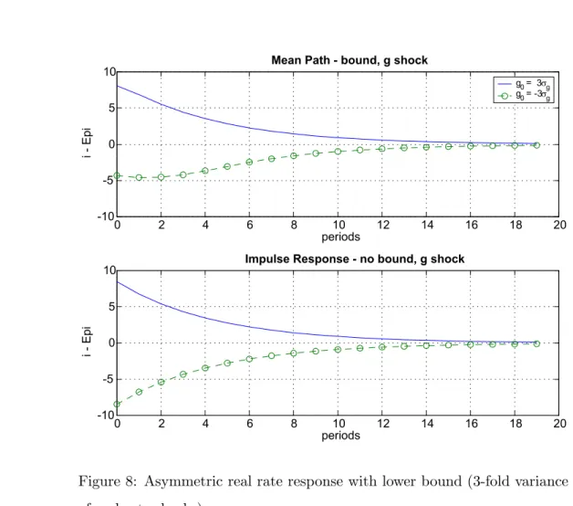
Figure 8 illustrates the mean response of the real rate to a ±3 standard deviation real rate shock under optimal policy. The upper panel shows the case with lower bound and the lower panel depicts the case without bound. While in the latter case the policy reaction is perfectly symmetric, imposing the bound creates a sizeable asymmetry: the real rate reduction in
2 6
In this paper we compute welfare losses by taking one thousand random draws of
the initial states(u0, g0, µ10, µ20)from their stationary distributions (under optimal policy
with and without lower bound) and then evaluate the corresponding welfare losses in the subsequent one thousand periods.
2 7
This value is roughly consistent with the estimated variability of real rate shocks in the period 1979:4-1995:2, i.e., the time span considered by Rotemberg and Woodford (1998). The unconditional variance of the real rate shocks for 1979:4-1995:2 is about 2.5-fold that for the period 1983:1-2002:4.
response to a negative shock is much weaker than the corresponding increase in response to a positive shock.28
Equation (3), however, implies that the policymaker is unable to affect the average real rate in any stationary equilibrium.29 Therefore, the less strong real rate decrease for a binding real rate shock has to be compensated with a less strong real rate increase (or a stronger real rate decrease) in response to other shocks. A close look atfigure 8 reveals that this is indeed the case: the real rate increase with the lower bound falls slightly short of the one implemented without bound.
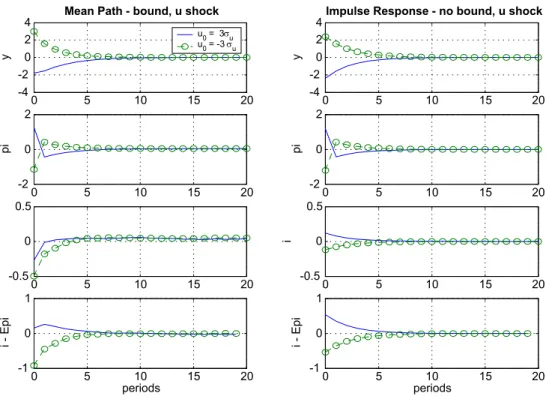
Moreover, it is optimal to undo the asymmetry by trading-off across all shocks, e.g., also across mark-up shocks. This is illustrated in figure 9 which plots the economy’s mean response to±3 standard deviation mark-up shocks. The left-hand panel illustrates the response when the zero lower bound is imposed and the right-hand panel depicts the case without bound. Clearly, the mean reactions change considerably once the lower bound is imposed. Real rates are now lowered more (increased less) in response to negative (positive) mark-up shocks. This is the case even though mark-up shocks do not lead to a binding lower bound.
8
We now analyze the robustness of our findings to a number of variations in our baseline calibration. Particular attention is given to the sensitivity of the results to changes in the parameterization of the shock processes.
2 8With negative shocks expected inflation has to be used to reduce the real interest rate
which is a costly instrument in welfare terms. 2 9
This can be seen by taking unconditional expectations of equation (3), imposing
sta-tionarity, and noting thatE[gt] = 0.
8.1
We estimated the shock processes using data for a time period that most economists would consider to be relatively ‘calm’ especially when confronted with the more ‘turbulent’ 1960s and 1970s. Since one cannot exclude that more ‘turbulent’ times might lie ahead, it seems to be of interest to study the implications of optimal policy with more variable mark-up and real rate shocks. In this regard, this section considers the sensitivity of ourfindings to an increase of the shock variancesσ2
u andσ2g above the values in table 1.
Increasing the variance of mark-up shocks we find that the results are remarkably stable. This holds even if setting the variance of σ2
u threefold
above its estimated value. Average output and (annual) inflation are vir-tually unaffected. Moreover, zero nominal rates still occur with the same frequency and persistence as for the baseline parameterization of table 1.
The picture changes somewhat increasing the variance of real rate shocks. While average output remains virtually unaffected, average inflation and the average frequency and persistence of zero nominal rates do change, albeit to different extents. This is illustrated in the first three panels offigure 10, that show the implications of increasing the variance of real rate shocks up to threefold above that of the baseline calibration.30 Average inflation and the average persistence of zero nominal rates change only in minor ways. Instead, as real rate shocks become more variable, zero nominal rates occur much more often.
Moreover, as can be observed in the lowest panel of figure 10, the addi-tional welfare losses generated by the zero lower bound increase markedly
3 0
This value is roughly consistent with the estimated variability of real rate shocks in the period 1979:4-1995:2, i.e., the time span considered by Rotemberg and Woodford (1998). The unconditional variance of the real rate shocks for 1979:4-1995:2 is about 2.5-fold that for the period 1983:1-2002:4.
with the variance of the real rate shock process. While for the baseline cali-bration the additional average losses of the zero lower bound over and above those generated by the stickiness of prices is in the order of 1%, once the variance of real rate innovations is threefold the additional losses surge to roughly 33%. This shows that the welfare effects of the zero lower bound are more sensitive to the variance of the assumed real rate process.
One should note that the effects of the variability of shocks on the average level of output and inflation differ considerably from those reported in earlier contributions. Uhlig (2000), e.g., reports negative level effects for both vari-ables when analyzing optimal policy in a backward-looking model. Clearly, the gains from promising positive values of future output and inflation can-not show up in a backward-looking model. Similarly, Coenen, Orphanides and Wieland (2004) report negative level effects for a forward-looking model considering Taylor-type interest rate rules, rather than optimal policy as in this paper. Moreover, unlike suggested by Summers (1991), our results do not justify that it is necessary to target positive inflation rates so as to safeguard the economy against hitting the zero lower bound.
8.2
Our benchmark calibration of table 1 assumes an interest rate elasticity of output of ϕ = 6.25, which seems to lie on the high side for plausible estimates of the intertemporal elasticity of substitution.31 Therefore, we
also consider the caseϕ= 1that corresponds to log utility in consumption, and constitutes the usual benchmark parameterization in the real business cycle literature. Table 2 presents the parameters values implied by assuming ϕ = 1 instead of ϕ = 6.25. Note that the values of λ and α are also
3 1As argued by Woodford (2003), a high elasticity value may capture non-modeled
interest-rate-sensitive investment demand.
changed, as they depend on the intertemporal elasticity of substitution.32 To estimate the shock processes, we follow the same procedure as for the baseline calibration. Details of the estimation are given in appendix A.3.
Overall, our findings seem robust to the change in the intertemporal elasticity of substitution. In particular, the level effects on average output and inflation remain negligible. Moreover, required inflation in response to a negative 3 standard deviation real rate shock is still in the order of 15 basis points annually. Even more importantly, the additional welfare losses generated by the zero bound are rather small and in the order of less than one-half percent of the losses generated by the stickiness of prices alone.
Respect to the baseline, however, the lower bound is binding more fre-quently, namely in about one quarter every 5 years on average. Binding real rate shocks occur more often because the variance of the real rate shock process implied by the parameterization in table 2 is about 45% higher than in our baseline.33 However, binding shocks now generate lower additional welfare losses: the steeper slopeλof the Phillips curve implies that inflation reacts more strongly to output. As a result, the required amount of inflation can be generated with less positive output gaps, implying lower additional welfare losses.
9
Conclusions
In this paper we determine optimal monetary policy under commitment tak-ing directly into account the zero lower bound on nominal interest rates and assess its quantitative importance for the U.S. economy. One of the main findings is that, given the historical properties of the estimated shock
pro-3 2
See equations (2.19) and (2.22) in chapter 6 of Woodford (2003). 3 3
Mark-up shocks also play a less marginal role, a negative shock in the order of 4 standard deviations now leads to a binding lower bound.
cesses for the U.S. economy, the zero lower bound seems neither to impose large constraints on optimal monetary policy nor to generate large addi-tional welfare losses. Furthermore, we show that the existence of the zero lower bound might require to lower nominal interest rates more aggressively in response to adverse shocks than what is suggested instead by a model without lower bound.
Ourfindings raise a number of further issues. First, the omission offiscal policy clearly constitutes a shortcoming; the study of the potential role of fiscal policy in ameliorating adverse welfare effects entailed by the lower bound seems to be of interest. Second, given the widespread belief among academics and practitioners that lagged inflation is a major determinant of inflation, an issue that should be addressed is the robustness of ourfindings to the introduction of lagged inflation in the Phillips curve.
Finally, the central bank’s credibility is key to our results. The use of expected inflation is unavailable to a discretionary policymaker, as there is no incentive to implement promised inflation ex-post. The zero lower bound on nominal interest rates, therefore, may generate significant additional wel-fare losses under discretionary policy. We explore this issue in a companion paper, see Adam and Billi (2003).
A
Appendix
A.1
Identi
fi
cation of historical shocks (baseline calibration)
To identify the historical shock processes we apply the procedure of Rotem-berg and Woodford (1998). In particular, we first construct output and inflation expectations by estimating expectation functions from the data. We then plug these expectations along with actual values of the output gap and inflation into equations (2) and (3), and identify the shocks ut and gt
We measure the output gap by linearly detrended log real GDP, and inflation by the log quarterly difference of the implicit deflator.34 Using quadratically detrended GDP or HP(1600)-filtered GDP leaves the esti-mated parameters of the shock processes virtually unchanged. Detrended output is depicted in figure 1. For the interest rate we use the quarterly average of the fed funds rate in deviation from the average real rate for the whole sample, which is approximately equal to3.5%(in annual terms). Based on this latter estimate we can set the quarterly discount factor as shown in table 1.
The expectation terms in equations (2) and (3) are constructed from the predictions of an unconstrained VAR in output, inflation, and the fed funds rate with three lags. Estimating expectation functions in such a way is justified as long as there are no structural breaks in the economy. Since our sample period, 1983:1-2002:4, starts after the disinflation policy under Federal Reserve Chairman Paul Volcker, monetary policy is expected to have been reasonably stable, see Clarida et al. (2000). A VAR lag order selection test based on the Akaike information criterion for a maximum of 6 lags suggests the inclusion of 3 lags. A Wald lag exclusion test indicates that the third lags are jointly significant at the 2% level. The correlations of the VAR residuals are depicted infigure 2. Substituting the expectations in equations (2) and (3) with the VAR predictions one can identify the shocks ut and gt. The implied shock series are shown infigure 3.
3 4
OLS estimates:
ρu= 0.129 (0.113)
ρg = 0.919 (0.050)
σu= 0.153
σg = 1.091
where numbers in brackets indicate standard errors. A univariate AR(1) describes the shock processesutand gtquite well. In particular, there is no
significant autocorrelation left in the innovations εi,t (i=u, g). Moreover,
when estimating AR(2) processes the additional lags remain insignificant. The estimated value of ρu is insignificant at conventional significance
levels. For this reason we set ρu = 0 and let the standard deviation of
the innovationsεu,tmatch the standard deviation of the identified mark-up
shocks, which is approximately equal to0.61%annually.
Although real rate shocks seem quite persistent, the persistence drops considerably once one uses actual future values to identify output and in-flation expectations in equations (2) and (3), which amounts to assuming perfect foresight. The estimated autoregressive coefficient for the real rate shocks then drops to ρg = 0.794, indicating that better forecasts than our
simple VAR-predictions would most likely lead to a reduction in the esti-mated persistence. Moreover, when using VAR-predictions but considering the period 1979:4-1995:2, as in Rotemberg and Woodford (1998), the point estimate falls toρg= 0.827. For these reasons we setρg= 0.8in our
calibra-tion.35 The standard deviation σg of the innovationsεg,t in table 1 equates
the unconditional standard deviation of the calibrated real shock process to the standard deviation of the identified shock values.
3 5This value cannot be rejected at the 1% significance level when using estimates based
on the VAR-expectations. In an earlier version of this paper, which is available upon
request, we used instead the point estimates forρuandρg.
A.2
Numerical algorithm
We use the collocation method to solve for the value function and the optimal policy functions in problem (9).36 In particular, one discretizes the state spaceS ⊂R4into a set ofN collocation nodesℵ={sn|n= 1, . . . , N}where
sn∈S. One then interpolates the value function over these collocation nodes
by choosing basis coefficientscn (n= 1, . . . , N) such that
W(sn) =
X
n=1,...,N
cnζ(sn) (11)
at each nodesn∈ ℵ, where ζ(·) is a four dimensional cubic spline function.
Equation (11) is an approximation to the left-hand side of (9).
To evaluate the right-hand side of (9) one has to approximate the ex-pected value EW(t(sn, x1, x2,ε)), where t(·) denotes the state transition function, x1 = (γ1,γ2) and x2 = (y,π, i) are the vectors of controls, and
ε= (εu,εg) are the multivariate normal innovations of the shock processes.
Assuming normality, the expected value function can be approximated by Gaussian-Hermite quadrature, which involves discretizing the shock distri-bution into a set of quadrature nodesεh and associated probability weights
ωh (h= 1, . . . , M).37
Substituting the collocation equation (11) for the value functionW(t(sn, x1, x2,ε)), the right-hand side of (9),RHSc(·), can be approximated as
RHSc(sn) = inf x1 sup x2 {h(sn, x1, x2) (12) +β X i=1,...,M X j=1,...,N ωicjζj(t(sn, x1, x2,εi))}
at each node sn ∈ ℵ. The maximization/minimization problem (12) can
be implemented using standard Newton methods, taking into account that 3 6
See chapter 11 in Judd (1998) and chapters 6 and 9 in Miranda and Fackler (2002) for more detailed expositions.
i≥ −r∗. This delivers RHSc(·) and the policy functions x1c(·) and x2c(·)
at the collocation nodes.
Using the collocation technique one can then approximate RHSc(·) by
a new set of basis coefficientsc0n (n= 1, . . . , N) such that
RHSc(sn) =
X
n=1,...,N
c0nζ(sn) (13)
at each nodesn∈ ℵ.
Equations (11), (12), and (13) together define the iteration
c→Φ(c) (14)
wherec is the initial vector of basis coefficients in (11) and Φ(c) the vector of basis coefficient c0 in (13). The fixed point of equation (9) satisfies c∗ =
Φ(c∗).
To solve for thisfixed point one proceeds as follows:
Step 1 Choose the degree of approximationN andM and appropriate collo-cation and quadrature nodes. Guess an initial basis coefficient vector c0.
Step 2 Iterate on equation (14) and update the basis function coefficient vec-torck tock+1.
Step 3 Stop and setc∗ =ck+1if¯¯ck+1−ck¯¯max<τ, whereτ >0is a tolerance level and |·|max denotes the maximum absolute norm. Otherwise go back to step 2.
Once the (approximate) fixed point c∗ has been found, one needs to assess the accuracy of the solution. Define the residual function
Rc∗(s) =RHSc∗(s)−
X
n=1,...,N
wheres∈ ℵεand ℵε is a grid of nodes for whichℵε∩ ℵ=∅. Then compute the maximum absolute approximation error
eabs = max
s∈ℵε|Rc∗(s)|
and the maximum absolute relative error
erel= max s∈ℵε ¯ ¯ ¯ ¯ ¯ ¯Rc∗(s)/ X n=1,...,N c∗nζ(s) ¯ ¯ ¯ ¯ ¯ ¯
For the baseline parameterization we set N = 6875 and M = 9, with relatively more nodes placed into the area of the state space where the policy functions display kinks. The support of the discretization is chosen so as to cover±4unconditional standard deviations of the exogenous states u and g, and to insure that in a long simulation of one million periods all state values fall inside the chosen support for µ1 and µ2. Since the latter can only be verified ex-post, i.e., after having obtained the solution, some experimentation is necessary to achieve this. Our initial guess for c0 is consistent with the solution of the problem without lower bound. The tolerance level is set to τ = 1.49 ·10−8, i.e., the square root of machine precision. Convergence is reached after about 39 hours on a Pentium IV with 2.6 GHz. The approximation errors areeabs= 0.0021anderel= 0.0027, whereℵε contained more than 75000 nodes.
A.3
Identi
fi
cation of historical shocks (RBC calibration)
We re-estimated the shock processes using the parameters from table 2 to-gether with VAR-based expectations, following the procedure described in appendix A.1. The autocorrelation coefficient for the mark-up shocks now turns out to be statistically significant at the 1% level. Therefore, in table 2 we setρu equal to its point estimate. The point estimate (standard
Since we still cannot rejectρg = 0.8 at conventional significance levels, we
keep this value of the baseline parameterization. As before, the standard deviation σg of the innovation εg,t is chosen so as to match the standard
deviation of the estimated real rate shocks.
References
Adam, Klaus and Roberto M. Billi, “Optimal Monetary Policy under
Discretion with a Zero Bound on Nominal Interest Rates,” University of Frankfurt Mimeo, 2003.
Auerbach, Alan J. and Marurice Obstfeld, “The Case for
Open-Market Purchases in a Liquidity Trap,” NBER Working Paper No. 9814, 2003.
Benhabib, Jess, Stephanie Schmitt-Grohé, and Martín Uribe,
“Avoiding Liquidity Traps,” Journal of Political Economy, 2002, 110, 535—563.
Buiter, Willem H. and Nikolaos Panigirtzoglou, “Overcoming the
Zero Bound on Nominal Interest Rates with Negative Interest on Cur-rency: Gesell’s Solution,”Economic Journal, 2003, 113, 723—746.
Calvo, Guillermo A., “Staggered Contracts in a Utility-Maximizing
Framework,” Journal of Monetary Economics, 1983, 12, 383—398.
Christiano, Lawrence J. and Jonas Fisher, “Algorithms for Solving
Dynamic Models with Occasionally Binding Constraints,” Journal of Economic Dynamic and Control, 2000, 24(8), 1179—1232.
Clarida, Richard, Jordi Galí, and Mark Gertler, “The Science of
Monetary Policy: Evidence and Some Theory,” Journal of Economic Literature, 1999,37, 1661—1707.
, , and , “Monetary Policy Rules and Macroeconomic Sta-bility: Evidence and Some Theory,” Quarterly Journal of Economics, 2000, 115, 147—180.
, , and , “Optimal Monetary Policy in Open versus Closed
Economies: An Integrated Approach,”American Economic Review Pa-pers and Proceedings, 2001, 91, 248—252.
Coenen, Günter and Volker Wieland, “The Zero-Interest-Rate Bound
and the Role of the Exchange Rate for Monetary Policy in Japan,”
Journal of Monetary Economics, 2003, 50, 1071—1101.
, Athanasios Orphanides, and Volker Wieland, “Price Stability and Monetary Policy Effectiveness When Nominal Interest Rates are Bounded at Zero,” Advances in Macroeconomics, 2004, 4(1) article 1.
Eggertsson, Gauti, “How to Fight Deflation in a Liquidity Trap: Com-mitting to Being Irresponsible,” IMF Working Paper 03/64, 2003.
and Michael Woodford, “Optimal Monetary Policy in a Liquidity Trap,” NBER Working Paper No. 9968, 2003.
Evans, George and Seppo Honkapohja, “Policy Interaction,
Expecta-tions and the Liquidity Trap,”mimeo, 2003.
Fuhrer, Jeffrey F. and Brian F. Madigan, “Monetary Policy When
Interest Rates Are Bounded at Zero,” Review of Economic Studies, 1997, 79, 573—585.
Goodfriend, Marvin, “Overcoming the Zero Bound on Interest Rate Pol-icy,”Journal of Money Credit and Banking, 2000,32 (4,2), 1007—1035.
Ireland, Peter, “Technology Shocks in the New Keynesian Model,” 2002. Boston College mimeo.
Judd, Kenneth L., Numerical Methods in Economics, Cambridge: MIT Press, 1998.
Jung, Taehun, Yuki Teranishi, and Tsutomu Watanabe, “Zero
Bound on Nominal Interest Rates and Optimal Monetary Policy,” 2001. Kyoto Institute of Economic Research Working Paper No. 525.
Kato, Ryo and Shin-Ichi Nishiyama, “Optimal Monetary Policy When
Interest Rates are Bounded at Zero,”Bank of Japan mimeo, 2003.
Krugman, Paul R., “It’s Baaack: Japan’s Slump and the Return of the Liquidity Trap,” Brookings Papers on Economic Activity, 1998,49(2), 137—205.
Marcet, Albert and Ramon Marimon, “Recursive Contracts,”
Univer-sitat Pompeu Fabra Working Paper, 1998.
and Wouter DenHaan, “Solving the Stochastic Growth by
Param-eterizing Expectations,” Journal of Business and Economic Statistics, 1990, 8(1), 31—34.
McCallum, Bennett T., “Japanese Monetary Policy, 1991-2001,”Federal Reserve Bank of Richmond Economic Quarterly, 2003, 89/1.
Miranda, Mario J. and Paul L. Fackler, Applied Computational
Eco-nomics and Finance, Cambridge, Massachusetts: MIT Press, 2002.
Orphanides, Athanasios, “Monetary Policy in Deflation: The Liquidity Trap in History and Practice,” Federal Reserve Board Mimeo, 2003.
and Volker Wieland, “Efficient Monetary Policy Design Near Price Stability,”Journal of the Japanese and International Economies, 2000,
Reifschneider, David and John C. Williams, “Three Lessons for Mon-etary Policy in a Low-Inflation Era,” Journal of Money Credit and Banking, 2000,32, 936—966.
Rotemberg, Julio J., “The New Keynesian Microfoundations,” NBER
Macroeconomics Annual, 1987,2, 69—104.
and Michael Woodford, “An Optimization-Based Econometric
Model for the Evaluation of Monetary Policy,” NBER Macroeconomics Annual, 1998,12, 297—346.
Schmitt-Grohé, Stephanie and Martín Uribe, “Optimal Simple and
Implementable Monetary and Fiscal Rules,” Duke University Mimeo, 2003.
Silberberg, Eugene,The Structure of Economics: A Mathematical Anal-ysis, New York: McGraw-Hill, 1990.
Summers, Lawrence, “Panel Discussion: Price Stability: How Should
Long-Term Monetary Policy Be Determined?,” Journal of Money Credit and Banking, 1991,23, 625—631.
Svensson, Lars E. O., “Escaping from a Liquidity Trap and Deflation: The Foolproof Way and Others,” Journal of Economic Perspectives, 2003, 17(4), 145—166.
Taylor, John B., “Discretion versus Policy Rules in Practice,” Carnegie-Rochester Conference Series on Public Policy, 1993,39, 195—214.
Uhlig, Harald, “Should We Be Afraid of Friedman’s Rule?,” Journal of Japanese and International Economies, 2000, 14, 261—303.
Wolman, Alexander L., “Real Implications of the Zero Bound on Nominal Interest Rates,” forthcoming Journal of Money Credit and Banking, 2003.
Parameter Economic interpretation Assigned value
β quarterly discount factor
³
1 +3.5%4 ´−1 ≈0.9913
α weight on output in the loss function 0.40482 = 0.003
λ slope of the Phillips curve 0.024
ϕ real rate elasticity of output 6.25
ρu AR-coefficient mark-up shocks 0
ρg AR-coefficient real rate shocks 0.8
σu s.d. mark-up shock innovations (quarterly %) 0.154
σg s.d. real rate shock innovations (quarterly %) 1.524
Table 1: Parameter values (baseline calibration)
Parameter Economic interpretation Assigned value
β quarterly discount factor
³
1 +3.5%4 ´−1 ≈0.9913
α weight on output in the loss function 0.007
λ slope of the AS curve 0.057
ϕ real rate elasticity of output 1
ρu AR-coefficient mark-up shocks 0.36
ρg AR-coefficient real rate shocks 0.8
σu s.d. mark-up shock innovations (quarterly %) 0.171
σg s.d. real rate shock innovations (quarterly %) 0.294
Table 2: Parameter values (RBC calibration)
-6 -4 -2 0 2 4 84 86 88 90 92 94 96 98 00 02
-.3 -.2 -.1 .0 .1 .2 .3 1 2 3 4 5 6 7 8 Cor(Y,Y(-i)) -.3 -.2 -.1 .0 .1 .2 .3 1 2 3 4 5 6 7 8 Cor(Y,PI(-i)) -.3 -.2 -.1 .0 .1 .2 .3 1 2 3 4 5 6 7 8 Cor(Y,I(-i)) -.3 -.2 -.1 .0 .1 .2 .3 1 2 3 4 5 6 7 8 Cor(PI,Y(-i)) -.3 -.2 -.1 .0 .1 .2 .3 1 2 3 4 5 6 7 8 Cor(PI,PI(-i)) -.3 -.2 -.1 .0 .1 .2 .3 1 2 3 4 5 6 7 8 Cor(PI,I(-i)) -.3 -.2 -.1 .0 .1 .2 .3 1 2 3 4 5 6 7 8 Cor(I,Y(-i)) -.3 -.2 -.1 .0 .1 .2 .3 1 2 3 4 5 6 7 8 Cor(I,PI(-i)) -.3 -.2 -.1 .0 .1 .2 .3 1 2 3 4 5 6 7 8 Cor(I,I(-i))
Figure 2: Residual autocorrelations with 2 s.d. error bounds for an unre-stricted VAR in GDP, inflation, and fed funds rate.
-.4 -.3 -.2 -.1 .0 .1 .2 .3 .4 .5 84 86 88 90 92 94 96 98 00 02 -6 -4 -2 0 2 4 6 8 84 86 88 90 92 94 96 98 00 02
u
tg
t-2 -1 0 1 2 -5
0
5 Optimal Policy, u shock
y bound no bound -10 -5 0 5 10 -5 0
5 Optimal Policy, g shock
y -2 -1 0 1 2 -2 0 2 pi -10 -5 0 5 10 -0.1 0 0.1 pi -2 -1 0 1 2 -0.2 0 0.2 i -10 -5 0 5 10 -10 0 10 i -2 -1 0 1 2 -1 0 1 gamma1 -10 -5 0 5 10 -0.04 -0.02 0 0.02 gamma1 -2 -1 0 1 2 -1 0 1 u gamma2 -10 -5 0 5 10 -0.03 -0.02 -0.01 0 g gamma2
-5.5 -5.4 -5.3 -5.2 -5.1 -5 -4.9 -4.8 -4.7 -4.6 -3.6 -3.5 -3.4 -3.3 -3.2 -3.1 -3 -2.9
-2.8 Optimal Policy, g shock
g
i
bound no bound
0 2 4 6 8 10 12 14 16 18 20 -2
0
2 Mean Path - bound, g shock
y g0 = 3σg g0 = -3σg 0 2 4 6 8 10 12 14 16 18 20 -0.2 0 0.2 pi 0 2 4 6 8 10 12 14 16 18 20 -5 0 5 i 0 2 4 6 8 10 12 14 16 18 20 -0.02 0 0.02 gamma1 0 2 4 6 8 10 12 14 16 18 20 -0.02 -0.01 0 gamma2 0 2 4 6 8 10 12 14 16 18 20 -5 0 5 periods i - Epi
1 2 3 4 5 6 7 8 9 10 11 0 0.1 0.2 0.3 0.4 0.5 0.6 0.7 0.8 0.9 Quarters Probability
0 2 4 6 8 10 12 14 16 18 20 -10
-5 0 5
10 Mean Path - bound, g shock
periods i - Epi g0 = 3σg g0 = -3σg 0 2 4 6 8 10 12 14 16 18 20 -10 -5 0 5
10 Impulse Response - no bound, g shock
periods
i - Epi
Figure 8: Asymmetric real rate response with lower bound (3-fold variance of real rate shocks)
0 5 10 15 20 -4
-2 0 2
4 Mean Path - bound, u shock
y u0 = 3σu u0 = -3σu 0 5 10 15 20 -4 -2 0 2
4Impulse Response - no bound, u shock
y 0 5 10 15 20 -2 0 2 pi 0 5 10 15 20 -2 0 2 pi 0 5 10 15 20 -0.5 0 0.5 i 0 5 10 15 20 -0.5 0 0.5 i 0 5 10 15 20 -1 0 1 periods i - Epi 0 5 10 15 20 -1 0 1 periods i - Epi
Figure 9: Mean response to±3 s.d. mark-up shock (3-fold variance of real rate shocks)
6 8 10 12 14 16 18 20 0
0.02 0.04
0.06 Average inflation (yearly rates)
Percentage points baseline
2Varg
3Varg
6 8 10 12 14 16 18 20
0 10
20 Frequency of zero nominal interest rates
Years baseline 2Varg 3Varg 6 8 10 12 14 16 18 20 1 1.5
2 Average persistence of zero nominal interest rates
Quarters baseline 2Varg 3Varg 6 8 10 12 14 16 18 20 1.5 2
2.5 Expected loss with and without lower bound
- Expected loss
Variance real rate shocks (%)
baseline
2Varg
3Varg bound
no bound