Anisotropic 3D texture synthesis with application to
volume rendering
Lasse Farnung Laursen Technical University of Denmark
Richard Petersens Plads Building 321 DK-2800 Kgs. Lyngby
Bjarne Kjær Ersbøll Technical University of Denmark
Richard Petersens Plads Building 305 DK-2800 Kgs. Lyngby
Jakob Andreas Bærentzen Technical University of Denmark
Richard Petersens Plads Building 321 DK-2800 Kgs. Lyngby
ABSTRACT
We present a novel approach to improving volume rendering by using synthesized textures in combination with a custom transfer function.
First, we use existing knowledge to synthesize anisotropic solid textures to fit our volumetric data. As input to the synthesis method, we acquire high quality images using a 12.1 megapixel camera.
Next, we extend the volume rendering pipeline by creating a transfer function which yields not only color and opacity from the input intensity, but also texture coordinates for our synthesized 3D texture. Thus, we add texture to the volume rendered images. This method is applied to a high quality visualization of a pig carcass, where samples of meat, bone, and fat have been used to produce the anisotropic 3D textures.
Keywords
Volumetric Rendering, Texture Synthesis, Transfer function.
1.
INTRODUCTION
The use of volumetric data is becoming increasingly common within research fields such as medical visualization, food production and graphics. This data is also ever increasing in size as the scanners providing the data, e.g. CT, MRI, and ultrasound scanners, are improving and thus able to provide higher resolutions. Increased precision and more detail is a natural evolution as having too much information, is somewhat of a luxury problem. When concerned with rendering volumetric data in real time, two issues persist. Firstly, the features that we would like to visualize might be on a finer scale than the voxels, despite the ever increasing amount of volume data. In our case, we visualize pig meat, and the variation in the texture of pig meat is on a finer scale than the resolution of our CT scan. Moreover, the voxels in our CT scanned data are stretched ten times along one axis. This problem is compounded by a second issue which is the fact that the CT intensities represent material density, which is not directly related to the appearance of the underlying tissue.
We present a novel approach which aims to alleviate both issues. With prior knowledge about the type of volumetric data we wish to visualize, we synthesize an anisotropic 3D texture which is applied to the volume data via a customized transfer function. Using this transfer function, we map the CT intensities to a high resolution solid pig meat texture which gives a qualitatively far better representation of the meat than any single color. Moreover, the solid texture texels are not stretched.
Solid textures are an ideal fit when rendering volumetric data. In almost all cases, there is an interest in rendering what is beneath the surface or subdividing the data to expose some deeper layer. Since a solid texture shares the same number of dimensions as common volume data, its application is relatively straightforward.
2.
Related Work
The focus of this paper can be divided into solid texture synthesis, and the application thereof in volumetric rendering.
Solid Texture Synthesis
Considerable work has been done within the field of texture synthesis, from parametric methods [HB95] to non-parametric methods [DB97, Har01], as well as alternative approaches [WL00]. Most texture synthesis algorithms use a sample texture as input, referred to from here on as exemplar. This exemplar forms the basis for either a parametric model, which synthesizes a new texture based on modeled Permission to make digital or hard copies of all or part of
this work for personal or classroom use is granted without fee provided that copies are not made or distributed for profit or commercial advantage and that copies bear this notice and the full citation on the first page. To copy otherwise, or republish, to post on servers or to redistribute to lists, requires prior specific permission and/or a fee.
parameters, or for a non-parametric algorithm, which reuses elements from the exemplar and recombines these to create a new, yet similar, texture.
Solid texture synthesis has been pioneered and expanded upon within the past two decades. Several methods, both parametric [GD95] and non-parametric [Wei02], as well as alternate approaches [JDR04], have been presented.
A recent texture synthesis method, which we use to create our anisotropic textures, is called texture optimization [KEBK05, KFCO+07]. This method iteratively improves the texture as a whole, making each modification smaller and more refined.
Volumetric Transfer Function
Volume rendering [DCH88] has come a long way. Most applications today make use of graphics hardware to improve performance [CN94]. The field has seen a dramatic increase of research into all kinds of visualization techniques involving volumetric data. Most volumetric data originates from either computed tomography or magnetic resonance scans, which do not yield a direct mapping to appearance attributes (i.e. color and texture of the scanned tissue). An obvious field of research is therefore to provide proper color and texture to this otherwise appearance deficient data. The visible human project is one such example, where a male and female body has been scanned, and subsequently cut and photographed to obtain the correlation between density and appearance. One method with which to color the data, is the use of a transfer function [HKRs+06a].
Many methods for creating transfer functions exist. From a simple pre-defined function capable of transforming between two number domains, to a user defined transfer function allowing for iterative refinement through user input [CS07]. In most cases, user input is desirable since the transfer function is often used as a tool to highlight or hide specific features in the volume data.
Other approaches include Dong and Clapworthy [DC05], who use 2D input exemplars to apply and synthesize texture to a volumetric volume simultaneously. By analyzing the orientation of each voxel in the volume data a patch based synthesis strategy is applied to apply and expand the 2D exemplar to the volume.
Lu et al. [LEQ+07] expand upon an existing 2D synthesis algorithm to create a flexible system for volume illustration. By extending the concept of Wang Cubes into the third dimension Lu et al. create a tileable solid texture set.
Manke and Wünsche [MW09] provide a formal framework for applying solid textures to a volume, similar to the work in this paper. They also present
methods for dealing with discontinuous mapping. In contrast to this paper, however they do not touch upon the scaling or periodicity issues of applying a repeating solid textures to a volume.
In this paper, we use a simple, piecewise constant transfer function which maps voxel intensities to entire texture volumes, similar to Manke and Wünsche [MW09]. Subsequently, the color values at the given position in the volume are obtained by lookup in these texture volumes. The voxel density is used as an indicator for opacity. The textures are applied in a multi-scale fashion to minimize the periodicity, which is further described in Section 6.
3.
Overview
It has been our overall goal is to improve the visualization of CT scanned data. By applying a solid texture to the data via a transfer function, we are able to increase the visual detail at a minor cost to the computations required.
We employ the texture optimization method presented by Kopf et al. [KFCO+07], to synthesize our anisotropic textures. There is a large overlap with our description and [KFCO+07]. This is partly to highlight particular details of our implementation and partly to make the present paper more self-contained. Unfortunately, the aforementioned texture synthesis method does a poor job of synthesizing textures with only low frequency features. This leads to some muscle textures being comparable to base noise textures with similar colors.
Due to computational limitations, synthesizing solids larger than 128x128x128 is not feasible. This presents a number of scale and periodicity issues which we explore in sections 6 and 7. In short, we apply the synthesized texture in multiple scales to allow for fine and rough effects. We still make use of the CT data to add additional rough detail.
The results of these iterative improvements are compared and discussed, also in section 7.
4.
Solid Texture Synthesis
As previously explained, texture optimization is an iterative method where the difference between the input exemplar and the synthesized solid is minimized. The difference is measured by a global texture energy function which compares fixed sized 8x8 2D neighborhoods. For now, let us assume that each voxel/texel defines its own neighborhood. We define a simplified global texture energy function, similar to the one by Kopf et al. [KFCO+07].
, = ,− ,
.
The neighborhoods in the synthesized solid and input exemplar(s), are denoted by and
The total number of number of neighborhoods from the synthesized solid () is denoted
vectorized neighborhood in the solid is denoted and its closest match (in norm)
exemplar(s), is denoted by ,
= 0.8 makes the function more robust against outliers [KFCO+07, KEBK05].
Initially, the synthesized volume is comprised of randomly selected texels from the input exemplar. The volume is then iteratively improved
the input exemplar(s). The process an expectation maximization algorithm.
the “best looking” parameters, then we optimize based on those findings, and repeat the process.
Figure 1: Exemplars on the three planes orthogonal to the main axes.
As mentioned previously, comparing the synthesized texture to the input exemplar(s) is done by comparing fixed sized 8x8 neighborhoods. These
are extracted from both the synthesized volume and the input exemplar(s). However, there is not previously mentioned - one neighborh
each voxel. Rather, each voxel is indirectly related to the neighborhoods that includes it.
Figure 2: Density of neighborhoods on both exemplar and synthesis textures.
The neighborhoods in the synthesized solid and input and respectively. The total number of number of neighborhoods from ) is denoted . The th vectorized neighborhood in the solid is denoted,, orm) in the input . The exponent makes the function more robust against Initially, the synthesized volume is comprised of from the input exemplar. The volume is then iteratively improved to resemble is comparable to an expectation maximization algorithm. We first find the “best looking” parameters, then we optimize based on those findings, and repeat the process.
Figure 1: Exemplars on the three planes orthogonal to the main axes.
As mentioned previously, comparing the synthesized texture to the input exemplar(s) is done by comparing fixed sized 8x8 neighborhoods. These neighborhoods are extracted from both the synthesized volume and However, there is not – as one neighborhood assigned to Rather, each voxel is indirectly related to
Figure 2: Density of neighborhoods on both exemplar and synthesis textures.
On the input exemplars, these neighborhoods lie on a densely populated grid, since we want to use all the available information provided to us
texture to be synthesized. In the synthesized volume the neighborhoods lie on a sparse grid
voxel apart like Kopf et al. [KFCO+07]
planes orthogonal to the three main axes of our coordinate system, as shown in F
to reduce computation time and avoid re issues.
Figure 2 visualizes the sparse grid upon which the synthesized neighborhoods lie. A given voxel highlighted in blue - is a member of 16 on any given plane, due to the sythesized solids toroidal boundary conditions.
Once the all the neighborhoods have the “best looking” parameters are
locating the least different neighborhood in the input exemplar(s), for each neighborhood in the synthesized volume. Once found, each voxel is assigned a new value based on
corresponding best matches of the neighborhoods overlapping that voxel. Essentially averaging all the contributions to make a new color:
=∑∈
Equation 2: Voxel color calculation.
The new color assigned to the voxel in the synthesized solid, denoted
several existing color values. The above equation states that for each neighborhood
member of, we find the matching texel matching neighborhood , !
divided by , which denotes the number of neighborhoods the voxel is a part of
Figure 3: Neighborhoods on the three planes orthogonal to the main axes matched to input
exemplar neighborhoods.
Figure 3 visualizes equation
sparsely populated grid on the synthesized solid, a single voxel is member of 16 neighborhoods on a single plane orthogonal to a main axis.
three such planes, visualized as blue, yellow, and green in figure 3, the voxel is a member of
48 neighborhoods. Each of these neighborhoods a corresponding match in an
overlapping the same position in each of these the input exemplars, these neighborhoods lie on a since we want to use all the information provided to us, about the texture to be synthesized. In the synthesized volume the neighborhoods lie on a sparse grid (spaced 1 [KFCO+07]), and only on planes orthogonal to the three main axes of our coordinate system, as shown in Figure 1. This serves to reduce computation time and avoid re-sampling Figure 2 visualizes the sparse grid upon which the synthesized neighborhoods lie. A given voxel – is a member of 16 on any given , due to the sythesized solids toroidal boundary Once the all the neighborhoods have been extracted, eters are then found by neighborhood in the input exemplar(s), for each neighborhood in the Once found, each voxel is assigned a new value based on texels in the sponding best matches of the neighborhoods overlapping that voxel. Essentially averaging all the contributions to make a new color:
,
.
Equation 2: Voxel color calculation.
The new color assigned to the voxel in the
, is an average of several existing color values. The above equation states that for each neighborhood the voxel is a member of, we find the matching texel , in the best !. This sum is finally , which denotes the number of
is a part of.
Figure 3: Neighborhoods on the three planes orthogonal to the main axes matched to input
exemplar neighborhoods.
visualizes equation 2 in practice. In our sparsely populated grid on the synthesized solid, a single voxel is member of 16 neighborhoods on a single plane orthogonal to a main axis. Since we have three such planes, visualized as blue, yellow, and voxel is a member of a total of 48 neighborhoods. Each of these neighborhoods has n exemplar. The texel overlapping the same position in each of these
neighborhoods contributes to the sum, which is eventually divided by the total number of contributions (in this case 48), yielding the new color.
The optimization algorithm is actually performed on multiple levels of differing quality. The synthesized solid initially consists of 32x32x32 voxels, and input exemplar(s) are scaled to 32x32 respectively. Once the synthesis process reaches certain conditions, outlined in section 4.5, the volume is scaled up to 64x64x64 using trilinear interpolation. Due to computational restrictions of performing a nearest neighbor search in a high dimensional space, the synthesis is only performed up to a resolution of 128x128x128.
Approximate Nearest Neighbor
In a standard-RGB texture, an 8x8 neighborhood consists of 192 values. Finding the nearest neighbor in a 192 dimensional space is a computationally expensive operation.
We apply the same optimizations as Kopf et al. [KFCO+07] to reduce the computation complexity. A principal component analysis is performed on the neighborhood vectors from the exemplar(s). By only preserving the coefficients required to maintain 95% of the variance, we can typically reduce the number of dimensions by half, or more.
We also employ the ANN: Approximate nearest neighbor library [MA10]. The library accepts a value
", and returns an approximate nearest neighbor guaranteed to be at most " + 1 away from the true nearest neighbor. We employ " = 2 as dictated by Kopf et al. [KFCO+07].
Weighting Scheme
As previously mentioned in section 4, using an exponent of 0.8 in equation 1, causes it to be more robust against outliers. However, minimizing the & norm is more cumbersome than minimizing the norm. So instead we introduce a weight into the equation and rewrite the terms of the energy function (1) to the following (similar to Kopf et al. [KFCO+07]):
,− ,
= ,− ,'(,− ,(
= ),,− ,
Equation 3: Energy function term re-write.
where ),= ,− ,'(. This leads to the following quadratic formula which we seek to minimize:
, = ),,− ,( *+,-!()
.
Equation 4: Improved energy function.
The weight parameter ), makes sure that the exemplar neighborhood closest to a given synthesized neighborhood, carries the most weight. Instead of a straight average as applied in equation 2, we are now calculating a weighted average which leads to the following formula when calculating a new voxel value:
=∑∑∈),) ,
,
∈ .
Equation 5: Weighted voxel color calculation.
Instead of dividing the sum by the total number of contributors, we now divide by the total amount of weight distributed among the contributions.
Meanshift
Although adjusting each contributing texel with a weight parameter yields better results and speeds up convergence, there are still numerous textures which fail to produces acceptable results. One persisting issue is that outliers still contribute to the final result, even if their contribution is minimal.
In order to minimize contribution from outliers, Kopf et al. [KFCO+07] employ a clustering approach, proposed by Wexler et al. [WSI07]. In short, every contributing texel is considered to be a cluster. These clusters are then merged depending whether their center is within a distance of 0 to one another. If any new clusters emerge, the process of searching and merging is repeated, until no further clusters form. Only texels from the dominant cluster end up contributing to the new voxel value.
The threshold 0 is decreased with each iteration over the course of a single resolution level convergence. Once the synthesized texture converges on a single level, the thresholding value 0 is reset. We found that setting 0 = 10, 0 = 0.05, and 0 = 0.01 worked well in many cases, on the lowest, medium, and highest resolution level, respectively.
Histogram Matching
The previously mentioned modifications to the original synthesis method, speeds up convergence and minimizes the impact of outliers. However, the algorithm will occasionally converge at certain minima, which fail to make full use of the exemplar(s) details.
Kopf et al. [KFCO+07] address this issue by utilizing histogram matching. The weight each texel carries is further adjusted, based upon whether its contribution will increase, or decrease, the similarity between the histograms of the input exemplar, and the
synthesized solid. Practically, they achieve this by keeping track of a 16-bin histogram for each of the input exemplars’ channels. Usually, this is just the red, green, and blue channel. Kopf et al. also note the importance of keeping this histogram up to date during each “maximization” phase. Otherwise, the method will just overshoot the intended histogram and overcompensate in the following iteration. When synthesizing anisotropic textures we maintain one histogram per input exemplar. We let each contributing texel pull in the direction of its exemplars histogram, which seems to work well. Just like Kopf et al. we also traverse the voxels in a random order, to avoid any directional bias.
Histogram matching is an integral part of creating the best results possible via texture optimization. It makes the algorithm take global statistics into consideration while still allowing for the use of a small neighborhood window. Histogram matching also speeds up convergence significantly.
Synthesis Convergence Conditions
We found that a fixed number of iterations yielded the best result with most textures (J. Kopf, pers. comm.). Iterating 100 times on the lowest resolution, 20 on the next level, and 10 on the highest level, worked well with most textures.
5.
Exemplar Acquisition
As with every other texture synthesis method, we require exemplars of the texture we intend to synthesize. Our exemplars were obtained using a 12.1 megapixel camera, Canon IXUS 120IS, in a well lit setting. Originally, we intended to obtain samples using a multispectral color and texture measurement vision system. This system measures up to 20 different bands across the visible and non-visible spectrum. These precise measurements are then combined to a final standard-RGB image. However, most household cameras actually yield more vivid and realistic colors as each sensor integrates a wider range of the spectrum than the more precise instrument.
6.
Rendering
To visualize the volumetric data, a simple ray casting technique [HKRs+06b] is applied using the GPU. To obtain the start and end point for each ray, two rendering passes are performed of a cube showing the front- and backface respectively. The cube acts as our rendering proxy and yields the start and end position for each ray, which is recorded into a buffer using the fragment shader.
An additional rendering pass is then performed where the fragment shader traces a ray through the space enclosed by the cube. The ray is traced with 0.001
increments in relation to the unit cube around the volume, and accumulates more color and opacity as it traverses the volume. The “ray-color” starts off black and completely transparent. For each step through the volume, the current density is classified as air, skin, fat, meat, or bone, according to the Hounsfield scale [Sev04]. Its contribution to the overall “ray-color” as well as “remaining transparency” is calculated by the following formulas:
234= 25∗ 7 ∗ 834∗ 85
25= 25∗ (1 − 85).
Equation 6: Color and transparency contribution per ray-step.
The contribution added to the existing color and transparency value of the ray is denoted as 234. The amount of contributing light via simple lambertian shading [HKRs+06c], is denoted 7. The contributing color and transparency from the classified density is denoted 834 and 85 respectively. When “ray-color” is completely opaque, the ray traversal is stopped.
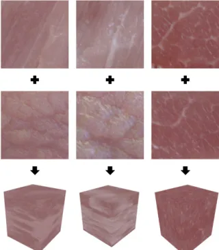
Figure 4: Three synthesized solids and their two input exemplars (pig muscle tissue). The left and middle synthesis’ yield an unsatisfactory result.
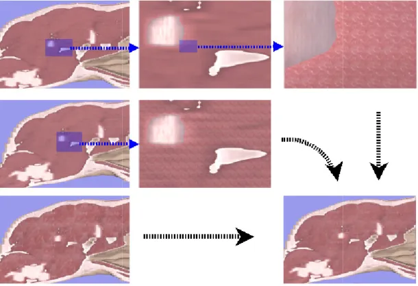
Setting 834 in Equation 6 to the color from the appropriately scaled solid texture produces a result with significant periodicity at high magnification and almost uniform color at low magnification (because of mipmapping). This can be seen in Figure 5, in the top and bottom left. To ameliorate these issues, we combine the texture at three levels of scaling, and
Figure 5: Three differently scaled muscle textures com
segment show zoomed in areas to show finer detail.
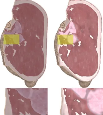
Figure 6: On the top, volumetric data from the pig carcass, visualized without enhanced graphics. The colors for the meat, bone, and fat tissue are the average color values of the textures applied on the right. On the bottom, volumetric data from the pig carcass, visualized with enhanced graphics. The highlighted
sections in yellow indicate the zoomed section displayed on th
Figure 5: Three differently scaled muscle textures combined to create the final result. The top and middle segment show zoomed in areas to show finer detail.
Figure 6: On the top, volumetric data from the pig carcass, visualized without enhanced graphics. The , bone, and fat tissue are the average color values of the textures applied on the right. On the bottom, volumetric data from the pig carcass, visualized with enhanced graphics. The highlighted
sections in yellow indicate the zoomed section displayed on the right.
bined to create the final result. The top and middle
Figure 6: On the top, volumetric data from the pig carcass, visualized without enhanced graphics. The , bone, and fat tissue are the average color values of the textures applied on the right. On the bottom, volumetric data from the pig carcass, visualized with enhanced graphics. The highlighted
834= 834 & 9&+ 8 34 9+ 9&+ 9+ 9 34= 834∗ :; − ;!<3 8=>-?@= 834+ 34
Equation 7: Density case color contribution.
The color contribution consists of three differently scaled textures 834&'A and an associated weight factor
9&'A. For each tissue, the scales differ approximately a factor of 10, and the weight factor is always highest for the macro texture (approximately 3 to 1). Density is contributed to the final color value
The value :; represents a scaled measure of the density at that point in the volumetric data, and
;!<3 <+@Bdenotes the density threshold of the contributing tissue. The result of combining the three synthesized muscle textures, along with the density modifier, is visualized in Figure 5.
An exception to the calculation outlined in Equation 7 is the skin color contribution which yields a constant average color of sampled pig skin, permeated by simplex noise [Per01] to give some variation to the surface.
The transparency value for either fat, muscle or bone is calculated via the following formu
85= max(0.3, :; + 0
Skin has a constant translucency of 0.75, and air is completely transparent.
7.
Results
We implemented the method described in this paper entirely in C++. The time required to generate a
128Asolid depends primarily on the size an
of the input exemplars. On an Alienware m17x model (using only a single core) the synthesis of our three tissue types would usually converge after approximately 2-3 hours. It was our experience that the algorithm generated the best textures when forcing two of the three dimensions to conform to input exemplars, regardless of whether isotropic anisotropic synthesis.
As previously mentioned in section 3, the synthesis algorithm has trouble synthesizing 3D textures based on input exemplars with primarily low frequency features. The two initial attempts in figure
how the final synthesized solid ends up looking almost nothing like the original two textures used as input. The third synthesized solid is much more promising.
A question of scale arises when choosing how much surface a single exemplar should cover. To ensure we acquired as homogenous a sample as possible, and preserve detail, we chose to use exemplars covering a small area of approximately 2x2 cm.
+ 834A 9A
9A 3 <+@B 34
Equation 7: Density case color contribution.
The color contribution consists of three differently and an associated weight factor . For each tissue, the scales differ approximately a factor of 10, and the weight factor is always highest for the macro texture (approximately 3 to 1). Density is contributed to the final color value 8=>-?@ via 34. represents a scaled measure of the density at that point in the volumetric data, and denotes the density threshold of the contributing tissue. The result of combining the three textures, along with the density outlined in Equation is the skin color contribution which yields a constant average color of sampled pig skin, permeated by simplex noise [Per01] to give some either fat, muscle or bone is calculated via the following formula:
0.25).
Skin has a constant translucency of 0.75, and air is
We implemented the method described in this paper The time required to generate a solid depends primarily on the size and richness of the input exemplars. On an Alienware m17x model (using only a single core) the synthesis of our three tissue types would usually converge after It was our experience that the algorithm generated the best textures when only forcing two of the three dimensions to conform to input exemplars, regardless of whether isotropic, or As previously mentioned in section 3, the synthesis algorithm has trouble synthesizing 3D textures based imarily low frequency The two initial attempts in figure 4 show how the final synthesized solid ends up looking almost nothing like the original two textures used as input. The third synthesized solid is much more scale arises when choosing how much surface a single exemplar should cover. To ensure we acquired as homogenous a sample as possible, and preserve detail, we chose to use exemplars covering a small area of approximately 2x2 cm.
As previously mentioned in section
value of a voxel is modified by a simple mapping of the current density. The density modifier allows for a number of low frequency details to show, as is visualized in Figure 7.
Figure 7: Two hams, with and without density value modification. The highlighted sections in yellow indicate the zoomed section displayed on
the bottom.
The final result of the visualized volume data with all the aforementioned techniques applied is shown in Figure 6.
Figure 8: The volume data rotation preliminary benchmark.
visualized.
We perform a preliminary benchmark of the applied synthetic textures by rotating the volume complete turn, around the y-axis
Std. Graphics Min. Fps
Max. Fps
Avrg. Fps 76.817
Table 1: Preliminary performance measurements.
The application of the synthesized textures only requires three additional texture lookups per ection 6, the final color value of a voxel is modified by a simple mapping of the current density. The density modifier allows for a number of low frequency details to show, as is
Figure 7: Two hams, with and without density modification. The highlighted sections in yellow indicate the zoomed section displayed on
the bottom.
The final result of the visualized volume data with all the aforementioned techniques applied is shown in
Figure 8: The volume data rotation pattern of the preliminary benchmark. Unenhanced pig
visualized.
We perform a preliminary benchmark of the applied synthetic textures by rotating the volume one axis, as seen in Figure 8. Std. Graphics Enh. Graphics
53 47
118 102
76.817 61.117
Table 1: Preliminary performance measurements.
The application of the synthesized textures only requires three additional texture lookups per
visualized voxel. Since texture lookups are implemented on the hardware level, it comes as no surprise that the performance loss is minimal
in Table 1. However, creating the synthesized textures is another matter. Due to the complexity of a nearest neighbor search in a high dimensional space, performing the synthesis in real
impossibility.
8.
Conclusion
s and Future Work
We have utilized an existing texture synthesis approach to produce three anisotropic textures were then applied to volumetric data transfer function, improving upon colorless data.
The technique can potentially be applied to any type of volumetric data and is not necessarily constricted to organic tissue.
Although the result has improved significantly, there is still room for improvement.
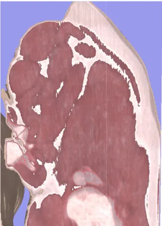
Figure 9: A close up of the visualized volumetric data showing computed tomography artifacts.
Our light model is simplistic. Better modeling of how light and meat interact would be an obvious next step since, recently, techniques for real
computation of translucent surfaces have started to appear, e.g. [WWH+10].
As mentioned in the previous section, we modify the final color slightly via the density of the volumetric data. While this adds significant detail to the final visualized voxel. Since texture lookups are hardware level, it comes as no surprise that the performance loss is minimal, as seen . However, creating the synthesized Due to the complexity of a nearest neighbor search in a high dimensional space, ynthesis in real-time is an
s and Future Work
utilized an existing texture synthesis anisotropic textures, which volumetric data via a custom upon the original The technique can potentially be applied to any type of volumetric data and is not necessarily constricted Although the result has improved significantly, there
close up of the visualized volumetric data showing computed tomography artifacts.
etter modeling of how light and meat interact would be an obvious next step since, recently, techniques for real-time interactive of translucent surfaces have started to As mentioned in the previous section, we modify the final color slightly via the density of the volumetric data. While this adds significant detail to the final
visualization, it also introduce
introduced by the scanning method. Figure 9 how the data acquisition rays from computed tomography leaves visible artifacts in the volume data.
Due to time required to perform a complete solid texture synthesis it could be advantageous to create a larger pre-computed library of multiple tissue types (in addition to the three described in this paper). Theoretically, it would also be possible to synthesize in-between textures by using an input exemplar from each tissue type, to smooth the transition between them. A few practical experiments are
how convincing the resulting solid textures
It would also be interesting to implement and compare the technique demonstrated by
[LEQ+07]. Using their extension to the wang cube model is also a way of avoiding periodicity in the applied texture.
9.
ACKNOWLEDGMENTS
We would like to thank Johannes Kopf for the invaluable correspondence during the development of this paper. We also extend our thanks to the anonymous reviewers in helping us improve on the paper. This research was supported in part by the Danish Meat Research Institute. The CT scan of the pig carcass was also kindly provided by the Danish Meat Research Institute.
10.
REFERENCES
[CJ06] Thierry Carrard and Manuel Juliachs, Bandwidth-efficient Hardware
Rendering for Large Unstructured Meshes, WSCG 2006, 14th International Conference in Central Europe on Computer Graphics, Visualization and Comput
CZECH REPUBLIC, JAN 30 169–176 (English).
[CN94] Timothy J. Cullip and Ulrich Neumann, Accelerating volume reconstruction with 3d texture hardware, Tech. report, Chapel Hill, NC, USA, 1994.
[CS07] Amit Chourasia and Jue
Data Centric Transfer Functions for High Dynamic Range Volume Data, WSCG 2007 International Conference in Central Europe on Computer Graphics, Visualization and Computer Vision, Plzen, CZECH REPUBLIC, JAN 29 01, 2007, pp. 9–15 (English).
[DB97] Jeremy S. De Bonet, Multiresolution sampling procedure for analysis and synthesis of texture images, SIGGRAPH ’97: Proceedings of the 24th annual conference on Computer graphics and interactive techniques (New York, NY, visualization, it also introduces a number of artifacts by the scanning method. Figure 9 shows how the data acquisition rays from computed tomography leaves visible artifacts in the volume Due to time required to perform a complete solid advantageous to create a computed library of multiple tissue types (in addition to the three described in this paper). Theoretically, it would also be possible to synthesize
between textures by using an input exemplar from o smooth the transition between w practical experiments are required to see ng the resulting solid textures would be. It would also be interesting to implement and compare the technique demonstrated by Lu et al. . Using their extension to the wang cube model is also a way of avoiding periodicity in the
ACKNOWLEDGMENTS
We would like to thank Johannes Kopf for the invaluable correspondence during the development of We also extend our thanks to the anonymous reviewers in helping us improve on the This research was supported in part by the Danish Meat Research Institute. The CT scan of the pig carcass was also kindly provided by the Danish
[CJ06] Thierry Carrard and Manuel Juliachs, efficient Hardware-Based Volume Unstructured Meshes, 14th International Conference in Central Europe on Computer Graphics, Visualization and Computer Vision, Plzen, CZECH REPUBLIC, JAN 30-FEB 03, 2006, pp. [CN94] Timothy J. Cullip and Ulrich Neumann, Accelerating volume reconstruction with 3d texture hardware, Tech. report, Chapel Hill, NC, [CS07] Amit Chourasia and Juergen R. Schulze, Data Centric Transfer Functions for High c Range Volume Data, WSCG 2007, 15th International Conference in Central Europe on Computer Graphics, Visualization and Computer Vision, Plzen, CZECH REPUBLIC, JAN 29-FEB
nglish).
[DB97] Jeremy S. De Bonet, Multiresolution sampling procedure for analysis and synthesis of texture images, SIGGRAPH ’97: Proceedings of the 24th annual conference on Computer graphics and interactive techniques (New York, NY,
USA), ACM Press/Addison-Wesley Publishing Co., 1997, pp. 361–368.
[DC05] Feng Dong and Gordon J. Clapworthy, Volumetric texture synthesis for nonphotorealistic volume rendering of medical data, The Visual Computer 21 (2005), 463–473.
[DCH88] Robert A. Drebin, Loren Carpenter, and Pat Hanrahan, Volume rendering, SIGGRAPH ’88: Proceedings of the 15th annual conference on Computer graphics and interactive techniques (New York, NY, USA), ACM, 1988, pp. 65–74. [GD95] D. Ghazanfarpour and J. M. Dischler,
Spectral analysis for automatic 3-d texture generation, Computers & Graphics 19 (1995), no. 3, 413 – 422.
[Har01] P Harrison, A non-hierarchical procedure for re-synthesis of complex textures, WSCG ‘ 2001, 9th International Conference on Computer Graphics, Visualization and Computer Vision, PLZEN, CZECH REPUBLIC, FEB 05-09, 2001, pp. 190–197 (English).
[HB95] David J. Heeger and James R. Bergen, Pyramid-based texture analysis/synthesis, SIGGRAPH ’95: Proceedings of the 22nd annual conference on Computer graphics and interactive techniques (New York, NY, USA), ACM, 1995, pp. 229–238.
[HKRs+06a] Markus Hadwiger, Joe M. Kniss, Christof Rezk-salama, Daniel Weiskopf, and Klaus Engel, Real-time volume graphics, pp. 81– 102, A. K. Peters, Ltd., Natick, MA, USA, 2006. [HKRs+06b] Markus Hadwiger, Joe M. Kniss,
Christof Rezk-salama, Daniel Weiskopf, and Klaus Engel, Real-time volume graphics,pp. 163– 185, A. K. Peters, Ltd., Natick, MA, USA, 2006. [HKRs+06c] Markus Hadwiger, Joe M. Kniss,
Christof Rezk-salama, Daniel Weiskopf, and Klaus Engel, Real-time volume graphics,pp. 114– 116, A. K. Peters, Ltd., Natick, MA, USA, 2006. [JDR04] Robert Jagnow, Julie Dorsey, and Holly
Rushmeier, Stereological techniques for solid textures, ACM Trans. Graph. 23 (2004), no. 3, 329–335.
[KEBK05] Vivek Kwatra, Irfan Essa, Aaron Bobick, and Nipun Kwatra, Texture optimization for example-based synthesis, SIGGRAPH ’05: ACM SIGGRAPH 2005 Papers (New York, NY, USA), ACM, 2005, pp. 795–802.
[KFCO+07] Johannes Kopf, Chi-Wing Fu, Daniel Cohen-Or, Oliver Deussen, Dani Lischinski, and Tien-Tsin Wong, Solid texture synthesis from 2d exemplars, ACM Transactions on Graphics
(Proceedings of SIGGRAPH 2007) 26 (2007), no. 3, 2:1–2:9.
[LEQ+07] Aidong Lu, David S. Ebert, Wei Qiao, Martin Kraus, and Benjamin Mora, Volume illustration using wang cubes, ACM Trans. Graph. 26 (2007).
[MA10] David M. Mount and Sunil Arya, Ann: A library for approximate nearest neighbor searching., http://www.cs.umd.edu/ mount/ANN/, 2010.
[MW09] Felix Manke and Burkhard C.Wuensche, Texture-enhanced direct volume rendering, Proceedings of the 4th International Conference on Computer Graphics Theory and Applications (GRAPP 2009) (Lisbon, Portugal), 2009, pp. 185–190.
[Per01] Ken Perlin, Noise hardware, In Real-Time Shading SIGGRAPH Course Notes (2001), Olano M., (Ed.)., 2001.
[RV06] Daniel Ruijters and Anna Vilanova, Optimizing GPU Volume Rendering, JOURNAL OF WSCG, 14th International Conference in Central Europe on Computer Graphics, Visualization and Computer Vision, Plzen Bory, CZECH REPUBLIC, JAN 30-FEB 03, 2006, pp. 9–16 (English).
[SC07] Sakurambo and John Cayley, 3d coordinate system, Image on the Internet, 2007.
[Sev04] El Sevier, Introduction to ct physics,
http://www.angelfire.com/nd/hussainpassu/Physic s_of_Computed_Tomography.pdf, 2004.
[Wei02] Li-Yi Wei, Texture synthesis by fixed neighborhood searching, Ph.D. thesis, Stanford, CA, USA, 2002, Adviser- Levoy, Marc.
[WL00] Li-Yi Wei and Marc Levoy, Fast texture synthesis using tree-structured vector quantization, SIGGRAPH ’00: Proceedings of the 27th annual conference on Computer graphics and interactive techniques (New York, NY, USA), ACM Press/Addison-Wesley Publishing Co., 2000, pp. 479–488.
[WSI07] Yonatan Wexler, Eli Shechtman, and Michal Irani, Space-time completion of video, IEEE Trans. Pattern Anal. Mach. Intell. 29 (2007), no. 3, 463–476.
[WWH+10] Yajun Wang, Jiaping Wang, Nicolas Holzschuch, Kartic Subr, Jun-Hai Yong, and Baining Guo, Real-time rendering of heterogeneous translucent objects with arbitrary shapes, Computer Graphics Forum 29 (2010), 497–506.