1
UC3M Working papers Departamento de Economía
Economics Universidad Carlos III de Madrid
15-10 Calle Madrid, 126
November, 2015 28903 Getafe (Spain)
ISSN 2340-5031 Fax (34) 916249875
DYNAMIC CONDITIONAL SCORE PATENT COUNT PANEL DATA MODELS
By Szabolcs Blazseka and Alvaro Escribanob,
a
School of Business, Universidad Francisco Marroquín, Guatemala
b
Department of Economics, Universidad Carlos III de Madrid, Spain
Abstract
We propose a new class of dynamic patent count panel data models that is based on dynamic conditional score (DCS) models. We estimate multiplicative and additive DCS models, MDCS and ADCS respectively, with quasi-ARMA (QARMA) dynamics, and compare them with the finite distributed lag, exponential feedback and linear feedback models. We use a large panel of 4,476 United States (US) firms for period 1979 to 2000. Related to the statistical inference, we discuss the advantages and disadvantages of alternative estimation methods: maximum likelihood estimator (MLE), pooled negative binomial quasi-MLE (QMLE) and generalized method of moments (GMM). For the count panel data models of this paper, the strict exogeneity of explanatory variables assumption of MLE fails and GMM is not feasible. However, interesting results are obtained for pooled negative binomial QMLE. The empirical evidence shows that the new class of MDCS models with QARMA dynamics outperforms all other models considered.
Keywords: patent count panel data models, dynamic conditional score models, quasi-ARMA model, research and development, patent applications.
JEL classification codes: C33, C35, C51, C52, O3.
Corresponding author. Telefonica Chair of Economics of Telecommunications. Department of Economics, Universidad Carlos III de Madrid, Calle Madrid 126, 28903, Getafe (Madrid), Spain. Telephone: +34 916249854 (Escribano). E-mail addresses: [email protected] (Blazsek); [email protected] (Escribano).
1. introduction
Patent activity and research and development (R&D) of firms were studied by the seminal works of Hausman, Hall, and Griliches (1984), Pakes (1985), and Jaffe (1986), who used panel data to investigate the relationships among input and output side measures of R&D activity, and various market value or accounting value based measures of firm performance. Other more recent works used dynamic patent count panel data models to study the relation-ships among patent counts, R&D and firm performance (Blundell, Griffith, and Windmeijer (2002); Wooldridge (2005); Blazsek and Escribano (2010), (2015); Bloom, Schankerman, and Van Reenen (2013)). In the present work we extend these models by suggesting a new class of dynamic patent count panel data models. By patent counts, we mean the number of success-ful patent applications of firms for a given year (Hausman, Hall, and Griliches (1984); Pakes (1985); Trajtenberg (1990); Lanjouw, Pakes, and Putnam (1998)). Although in recent patent databases the application date of patents is available with daily precision, this information is a noisy measure of the time of innovations. Therefore, following Hausman, Hall, and Griliches (1984), we aggregate patent counts over the year.
Harvey (2013, Chapter 5) noted that promising observation-driven time-series models of count data are the dynamic conditional score (DCS) Poisson models. In DCS Poisson models the dynamic equation is updated by the conditional score of the log-likelihood (LL) function, and the score is with respect to the time-varying conditional hazard parameter. The conditional score in these models discounts outliers and hence improves model fit. Harvey (2013) demonstrates the asymptotic theory of the maximum likelihood estimator (MLE) for different DCS models. These are location and scale DCS models for unrestricted and non-negative univariate continuous dependent variables, and multivariate DCS models for location, correlation and copula-based association. However, according to Harvey (2013, Section 5.11), the regularity conditions for the asymptotic distribution of MLE are not satisfied for DCS count data models based on the Poisson distribution.
time-series models for firm-level panels of patent count data. These are the multiplicative DCS (MDCS) and additive DCS (ADCS) patent count panel data models. For both DCS models we consider quasi-ARMA (QARMA) dynamics (Harvey (2013)). In order to demonstrate the advantages of the new DCS count models, we compare them with the finite distributed lag (FDL) model (Hausman, Hall, and Griliches (1984)), exponential feedback model (EFM) (Wooldridge (2005)) and linear feedback model (LFM) (Blundell, Griffith, and Windmeijer (2002)). We estimate all models for the extended panel dataset of patent applications used by Blazsek and Escribano (2010, 2015). This panel dataset includes 4,476 US firms for period 1979 to 2000. Related to the statistical inference, we consider the advantages and disadvantages of alternative estimation methods: MLE, pooled negative binomial quasi-MLE (QMLE) and generalized method of moments (GMM). For the count panel data models of this paper the strict exogeneity assumption maintained in MLE fails and GMM is not feasible. Nevertheless, interesting empirical results are obtained by the pooled negative binomial QMLE for which the asymptotic distribution of parameter estimates is known (Wooldridge (1997a), (2002)). We test whether R&D expenditure was exogenous for each model, and we also compare the statistical performance of different models by the Pearson squared and deviance residual R-squared metrics (Cameron and Windmeijer (1996)). The results suggest that MDCS-QARMA is superior to FDL, EFM, LFM and ADCS-QARMA.
The remainder of this paper is organized as follows. Section 2 presents the firm-level panel dataset. Section 3 presents econometric modeling and statistical inference. Section 4 summarizes diagnostic tests and empirical results. Section 5 concludes.
2. data
Griliches (1990) states that the main advantages of patent data are the following: (i) by definition, patents are closely related to inventive activity; (ii) patent documents are objective because they are produced by an independent patent office and their standards change slowly over time; (iii) patent data are widely available in several countries over long periods of time and cover almost every field of innovation. Lanjouw and Schankerman (1999) and Hall, Jaffe,
and Trajtenberg (2001) also validate the use of patent statistics in economic research. We perform all data procedures according to the recommendations suggested by Hall, Jaffe, and Trajtenberg (2001). The source of the US utility patent dataset of this study is MicroPatent LLC. The US patent database includes the USPTO patent number, application date, publication date, USPTO patent number of cited patents, three-digit US technological class and company name (if the patent was assigned to a firm) for each patent. We use the application date to determine the time of an innovation, since inventors have incentive to apply for a patent as soon as possible after completing an innovation (Hall, Jaffe, and Trajtenberg (2001)). Company specific information is from Standard & Poor’s (S&P) Compustat data files. For each firm, we use the book value for the sample midpoint year (Hausman, Hall, and Griliches (1984)) and R&D expenses for each year. We created a match file and crossed the patent dataset with the firm dataset via the six-digit Compustat CUSIP codes. Firm-specific data are corrected for inflation by using consumer price index (CPI) data (source: US Department of Labor, Bureau of Labor Statistics). The sample includes 488,149 US utility patents with application dates for period 1979 to 2000 (T = 22 years) of 4,476 US firms (N = 4,476). These data represent a case for which the cross-sectional dimension of the panel N is large, relative to its time-series dimension T. Therefore, we use the asymptotic theory presented by Wooldridge (1997a, 2002) for the estimation of count panel data models.
3. econometric modeling and statistical inference
3.1. General Notation of Variables
We observe a panel of patent application counts and other firm-specific variables of i = 1, . . . , N randomly selected firms for yearst= 1, . . . , T. nitdenotes the annual patent application
count of firmiat periodt;rditdenotes the log of inflation adjusted R&D expenditure of firmiat
periodt;Di takes the value one for firms in the drug, computer, scientific instrument, chemical
and electronic components industries (high-tech industries), and zero otherwise; firm size bi is
model we summarize the explanatory variables by the vector Xit for firm i and period t. For
each model we present the components of Xit in the following section.
3.2. Parameter Estimation by ML
Hausman, Hall, and Griliches (1984) use the ML method to estimate the parameters of their patent count panel data models that include random effects (RE) or fixed effects (FE). We denote both RE and FE by αi. MLE maintains the following assumptions:
(ML1) nit|(Xi1, . . . , XiT, αi) ∼ Poisson(λit), where λit = λ(Xit, θ) is the conditional hazard
parameter of the Poisson distribution. This implies strict exogeneity of all explanatory variables, conditional on αi.
(ML2) λit is modeled by the exponential function: λit = λ(Xit, θ) = exp(Xitβ + lnαi) =
exp(Xitβ)αi.
(ML3) nit|(Xi1, . . . , Xit, αi) and nis|(Xi1, . . . , Xis, αi) fort 6=s are independent.
(ML4) αi is independent and identically distributed (i.i.d.) with Gamma(1,δ) distribution.
This implies that E(αi) = 1 and Var(αi) = δ.
MLE is given by those parameters that maximize LL of the patent application count time series, i.e., ˆθ = arg maxθLL(ni1, . . . , niT;θ). For RE MLE, (ML1) to (ML4) are maintained, thus αi
is assumed to be independent of Xit. For FE MLE, (ML1) to (ML3) are maintained, hence
α1, . . . , αN are not treated as latent i.i.d. variables, but rather as constant parameters. As a
consequence, the coefficients of time-constant explanatory variables are not identified and αi is
possibly not independent ofXit. If the assumptions maintained hold, then the ML method will
provide an efficient estimator (Wooldridge (1997a)).
In the following, we present LL for RE MLE and FE MLE. First, for patent count data models with RE, the marginal density of (nit|Xi1, . . . , Xit) can be obtained by integrating out
αi from the joint density of (nit, αi|Xi1, . . . , Xit), as follows: (3.1) f(nit|Xi1, . . . , Xit) = Z ∞ 0 exp(−λit)λnitit nit! ×δ δαδ−1 i exp(−δαi) Γ(δ) dαi,
where Γ is the gamma function. The integrand of this equation is the product of the condi-tional probability mass function ofnit|(Xi1, . . . , Xit, αi)∼Poisson(λit) and the marginal density
function of αi ∼ Gamma(1,δ). Under (ML2), equation (3.1) can be written as
(3.2) f(nit|Xi1, . . . , Xit) = δδ[exp(X itβ)]nit nit!Γ(δ) Z ∞ 0 exp{−αi[exp(Xitβ) +δ]}αinit+δ−1dαi.
In order to evaluate the integral we use the formula
(3.3)
Z ∞
0
exp(−ax)xbdx= Γ(b+ 1) ab+1 .
We substitutex=αi, a= exp(Xitβ) +δ and b=nit+δ−1 into equation (3.3) and obtain
(3.4) f(nit|Xi1, . . . , Xit) = δδ[exp(X itβ)]nit nit!Γ(δ) × Γ(nit+δ) [exp(Xitβ) +δ]nit+δ .
Hence, LL for the exponential patent count data model with RE is
(3.5) LL(Xi1, . . . , XiT, θ) = PN i=1 PT t=1lit(θ) = PN i=1 PT t=1δln(δ) +nit(Xitβ) + ln Γ(nit+δ)−ln Γ(δ)−(nit+δ) ln[exp(Xitβ) +δ].
From equation (3.5) we excluded−ln(nit!), since it does not depend on the parameters. Second,
for exponential patent count data models with FE the conditional hazard parameter is λit =
exp(Xitβ)αi. This gives the following form of LL under (ML1):
(3.6) LL(Xi1, . . . , XiT, θ) = PN i=1 PT t=1[nitlnλit−ln(nit!)−λit] =PN i=1 PT t=1[nit(Xitβ+ lnαi)−ln(nit!)−exp(Xitβ+ lnαi)].
We can approximate FE αi by solving the first-order condition ∂LL/∂(lnαi) = 0 that gives (3.7) αi = PT t=1nit PT t=1exp(Xitβ) .
We substitute this result into equation (3.6) and introduce the notation
(3.8) pit = exp(Xitβ)/ " T X s=1 exp(Xisβ) # .
Under this notation, LL for the exponential patent count data model with FE is
(3.9) LL(Xi1, . . . , XiT, θ) = N X i=1 T X t=1 lit(θ) = N X i=1 T X t=1 " nitln pit T X s=1 nis ! −pit T X s=1 nis # .
From equation (3.9) we excluded−ln(nit!), since it does not depend on the parameters.
Haus-man, Hall, and Griliches (1984) note that this LL is conditional on the sum of the number of patents in the sample, i.e., PT
s=1nis. The asymptotic variance of ˆθ for both RE MLE and
FE MLE is given by A−1BA−1/N. This is due to the following result shown by Wooldridge
(1997a, 2002): √N(ˆθ −θ) →d N(0, A−1BA−1), where A = E[−Hi(θ)]; B = E[si(β)si(β)0];
Hi(θ) = PT t=1∇θsit(θ); si(θ) = PT t=1sit(θ) = PT
t=1∇θlit(θ). Moreover, sit(θ) denotes the score
with respect to θ for observation nit, and lit for RE MLE and FE MLE is given by equations
(3.5) and (3.9), respectively. Consistent estimators of A and B are given by sample averages. In the following we present the reasons why MLE is probably not the most adequate esti-mation method for the count data models of this paper. First, for the FDL model k lags of R&D are considered, Xit = (1, Di, bi, rdit, . . . , rdit−k). For EFM and LFM, Xit also includes
the first lag of patent count and the initial condition, Xit = (1, nit−1, ni1, Di, bi, rdit, . . . , rdit−k).
For all DCS count panel data models, Xit includes several lags of the conditional score
vari-able uit instead of the first lag of patent count. For example, for MDCS-QMA(q), Xit =
(1, uit−1, . . . , uit−q, ni1, Di, bi, rdit, . . . , rdit−k). In all these models, the strict exogeneity
expenditure. For EFM and LFM, (ML1) fails since the first lag of patent countnit−1 is included
as explanatory variable. For DCS count data models (ML1) fails since the conditional score uit is a transformation of the patent count nit, hence DCS models also include lagged patent
counts in the model specification. Second, MLE assumes that unobserved effectsαi are included
in λit. For the DCS count panel data models considered in this paper, LL is not available in
closed form when unobserved effects are included in λit. This is due to the fact that lags of λit
appear in Xitβ, within the conditional score terms. This motivates the application of pooled
panel data models for which unobserved effects are not considered in the model formulation. As MLE may not be a consistent estimator of parameters for the count panel data models of this paper, therefore the pooled negative binomial QMLE (Wooldridge (1997a), (2002)) or GMM (Chamberlain (1992); Wooldridge (1997b)) estimators that do not require strict exogeneity of all explanatory variables, are possibly more adequate.
3.3. Multiplicative Exponential Count Panel Data Models
All models presented in this section are formulated forE(nit|Xi1, . . . , Xit) =λit = exp(Xitθ).
For this functional form of the conditional mean, the explanatory variables and the error term are multiplicative. In this section, we review the pooled FDL model (Hausman, Hall, and Griliches (1984)) and its extension, the pooled EFM (Wooldridge (2005)). In these models we do not condition on unobserved effects αi in the count data model, thus we consider pooled
count panel data models. The pooled FDL model (Hausman, Hall, and Griliches (1984)) is
(3.10) λit = exp(Xitθ) = exp[µ0+γ1t+γ2(t×rdit) +γ3Di+γ4bi+β5(L)rdit],
where t is linear time trend;Di indicates if the firm is in a high-tech industry; bi measures firm
size; β5(L) =
P5
k=0βkLk is the lag polynomial of five lags, which captures contemporaneous and
lagged impact of R&D expensesrdit on patent counts.
conditional hazard and controls the initial conditionni1 of the dynamic process, as follows:
(3.11) λit = exp(Xitθ) = exp[µ0+γ1t+γ2(t×rdit) +γ3Di+γ4bi+γ5ni1+β5(L)rdit+φ1nit−1]
3.4. Multiplicative DCS Count Panel Data Models
We propose a new formulation for the conditional expectation of patent count. The MDCS count data model is formulated for E(nit|Xi1, . . . , Xit) = λit = exp(Xitθ). This implies that
MDCS is also a multiplicative count panel data model, and we do not condition on unobserved effects αi in the conditional expectation of patent count. MDCS involves lags of the dynamic
term uit, which is defined as follows:
(3.12) uit = nit−λit λit = nit λit −1.
The same innovation term is suggested by Davis, Dunsmuir, and Streett (2003, 2005) and Harvey (2013, Section 5.11), who propose the DCS Poisson model for time-series data and estimate it by the ML method. They defineuitaccording to equation (3.12), since it coincides with the DCS of
the Poisson LL with respect to the conditional hazard parameterλit. This can be demonstrated
as follows. The conditional probability mass function of the Poisson random variable with conditional expectation λit is
(3.13) f(nit|Xi1, . . . , Xit) =
exp(−λit)λnitit
nit!
.
The partial derivative of the log of this function with respect to λit is
(3.14) ∂lnf(nit|Xi1, . . . , Xit) ∂λit
= nit λit
−1 = uit.
In a time-series framework Davis, Dunsmuir, and Streett (2003, 2005) and Harvey (2013, Section 5.11) suggest using uit as innovation term for the DCS Poisson model. Furthermore, Harvey
(2013) also suggests DCS time-series models with first-order autoregressive formulation. Ac-cording to these a possible first-order count panel data model would be
(3.15) λit =λ(Xit, θ) = exp(Xitθ) = exp(φ1lnλit−1 +θ1uit−1+Yitθ)˜
with |φ1|<1 for covariance stationarity, θ= (φ1, θ1,θ) and˜
(3.16) Yitθ˜=µ0+γ1t+γ2(t×rdit) +γ3Di+γ4bi+γ5ni1+β5(L)rdit.
Harvey (2013, p. 37, Theorem 1) demonstrates the information matrix for general first-order DCS models. Unfortunately, the conditions of this theorem do not hold for the first-order DCS Poisson model of equations (3.15) and (3.16). For time-series data Davis, Dunsmuir, and Streett (2003, 2005) use an alternative specification for the conditional mean ofnitby considering
several lags of uit, but they do not include autoregressive terms in their model. These authors
derive the information matrix for MLE and show that there exists an asymptotic distribution of MLE. Nevertheless, Harvey (2013, Section 5.11) notes that the central limit theorem is currently unavailable for MLE for this model. Based on Davis, Dunsmuir, and Streett (2003, 2005), the MDCS count panel data model is
(3.17) λit =λ(Xit, θ) = exp(Xitθ) = exp(Ψit+Yitθ)˜
(3.18) Ψit+1 =θ0uit+θ1uit−1+. . .+θquit−q,
where θ = (θ0, . . . , θq,θ). Following the terminology of Harvey (2013, p. 63), we name this˜
model MDCS-Quasi-MA(q) or MDCS-QMA(q). We also define a more compact formulation with infinite lags of uit by the next MDCS-QAR(1) model:
(3.20) Ψit+1 =φ1Ψit+θ0uit,
where |φ1|<1 and θ = (φ1, θ0,θ). Furthermore, we combine the previous models to obtain the˜
following MDCS-QARMA(p,q) model:
(3.21) λit =λ(Xit, θ) = exp(Xitθ) = exp(Ψit+Yitθ)˜
(3.22) Ψit+1 =φ1Ψit+. . .+φpΨit−p+θ0uit+θ1uit−1+. . .+θquit−q.
3.5. Additive DCS Count Panel Data Models
The previous count data models with exponential conditional mean function assume a multi-plicative form of the conditional expectation of patent count. Nevertheless, there are several al-ternative formulations of the conditional mean of patent count in the literature. Examples are the Box-Cox-like model (Wooldridge (1997a)) and LFM (Blundell, Griffith, and Windmeijer (2002)). All additive count panel data models of this section are formulated forE(nit|Xi1, . . . , Xit) =λit.
This implies that we do not condition on unobserved effects αi in the conditional expectation
of patent count. We start with the pooled LFM, which is specified as
(3.23) λit =λ(Xit, θ) = φ1nit−1 + exp(Yitθ),˜
where 0< φ1 <1 andθ = (φ1,θ).˜ Yitθ˜is defined in equation (3.16). In the following, we propose
several ADCS specifications. The ADCS-QMA(q) count panel data model is
(3.24) λit =λ(Xit, θ) = Ψit+ exp(Yitθ)˜
(3.25) Ψit+1 =θ∗+θ0uit+θ1uit−1+. . .+θquit−q,
where θ∗ =θ0+. . .+θq and θ = (θ0, . . . , θq,θ). We include˜ θ∗ in equation (3.25) to ensure the
with infinite lags of uit, is the following ADCS-QAR(1) model:
(3.26) Ψit+1 =θ0+φ1Ψit+θ0uit,
where |φ1| < 1 and θ = (φ1, θ0,θ). We include˜ θ0 as constant parameter in equation (3.26) to
ensure the positivity of λit. Finally, we also define a more general dynamic formulation, the
ADCS-QARMA(p,q) model, as follows:
(3.27) Ψit+1 =θ∗+φ1Ψit+. . .+φpΨit−p+θ0uit+θ1uit−1 +. . .+θquit−q,
where θ∗ =θ0+. . .+θq and θ = (φ1, . . . , φp, θ0, . . . , θq,θ).˜
3.6. Parameter Estimation by QML
In this section, we present the details of the pooled negative binomial QMLE method. We use the methodology presented by Wooldridge (1997a, Sections 4.2 and 9.2; 2002, Section 19.6). The main advantage of the pooled negative binomial QMLE estimator with respect to MLE is that it requires weaker assumptions for consistent estimation. First, MLE assumes a specific conditional distribution of patent count that is not needed for the pooled negative binomial QMLE. Second, MLE assumes strict exogeneity for all explanatory variables that may fail, for example, due to lagged dependent variables included as explanatory variables, or due to feedback effects of past patent counts on future R&D expenses. Nevertheless, the pooled negative binomial QMLE can consistently estimate models with lagged dependent variables or other variables that are not strictly exogenous explanatory variables (Wooldridge (1997a)). Third, the pooled negative binomial QMLE does not consider αi in the model specification. In the count data models
estimated by this method E(nit|Xi1, . . . , Xit) = λ(Xit, θ) = λit, hence we do not condition on
αi. This is useful for both DCS count panel data models, where LL is not available in closed
form due to the latent αi term withinXitβ.
with RE for the case when the conditional distribution of patent count is Poisson and αi has
gamma distribution. A well-known choice for the parameters of gamma distribution for αi is
Gamma(1, δ). By integrating out RE from the joint density of patent count and RE, we obtain a negative binomial probability specification of the second kind that coincides with the objective function of the negative binomial QMLE (Hausman, Hall, and Griliches (1984); Cameron and Trivedi (1986); Wooldridge (1997a)). Furthermore, the use of the log negative binomial proba-bility mass function as objective function in QMLE is also motivated by Gourieroux, Monfort, and Trognon (1984a, b), who demonstrate that the negative binomial distribution with fixed value of δ is in the linear exponential family (LEF) of distributions. Gourieroux, Monfort, and Trognon (1984a, b) show that QMLE is a consistent estimator for LEF, provided that the con-ditional mean of the dependent variable is correctly specified. For the pooled negative binomial QMLE we assume that
(QMLE1) The conditional mean of patent count is correctly specified, i.e.,E(nit|Xi1, . . . , Xit) =
λ(Xit, θ) = λit. This implies the weak exogeneity (Cameron and Trivedi (2005)) of all
explanatory variables.
We implement the QMLE procedure (Gourieroux, Monfort, and Trognon (1984a, b)) following the two-step approach suggested by Wooldridge (1997a, Sections 4.2 and 9.2). In the first step, the δ parameter of the negative binomial distribution is estimated. In the second step, ˆδ is included into LL of the negative binomial distribution and QMLE is performed to estimate θ. The separate estimation of δ and θ is motivated by Gourieroux, Monfort, and Trognon (1984a, b). The details of the two-step QMLE negative binomial procedure are as follows. In the first step, the quasi-log-likelihood objective function for the pooled Poisson estimation is
(3.28) LL(Xi1, . . . , XiT, θ) = N X i=1 T X t=1 nitlnλ(Xit, θ)−λ(Xit, θ) = N X i=1 T X t=1 nitln(λit)−λit.
The pooled Poisson QMLE, denoted by ˆθ, maximizes LL. Gourieroux, Monfort, and Trognon (1984a, b) show that the Poisson distribution is LEF, hence the Poisson QMLE is a consistent
estimator under correct specification of the conditional mean of patent count. We define the Poisson residuals by ˆuit = nit−λ(Xit,θ), and also define the weighted (or Pearson) residualsˆ
by ˜uit = ˆuit/
q
λ(Xit,θ). Given these residuals, we estimateˆ δ by pooled ordinary least squares
(OLS) for the following linear regression model (Wooldridge, 1997a, Section 9.2):
(3.29) ˜u2it−1 = c+δλ(Xit,θ) +ˆ it
for i = 1, . . . , N and t = 1, . . . , T. The pooled OLS provides ˆδ, which we substitute into LL of the second step. In the second step, the quasi-log-likelihood objective function for pooled negative binomial estimation is
(3.30) LL(Xi1, . . . , XiT,ˆδ, θ) = N X i=1 T X t=1 ˆ δ−1ln " ˆ δ−1 ˆ δ−1 +λ(X it, θ) # +nitln " λ(Xit, θ) ˆ δ−1+λ(X it, θ) # .
The pooled negative binomial QMLE, denoted by ˆθ, maximizes LL. Gourieroux, Monfort, and Trognon (1984a, b) show that the negative binomial distribution is LEF. Therefore, the pooled negative binomial QMLE is consistent under correct specification of the conditional mean of patent count.
The asymptotic variance of ˆθis estimated by the following robust estimator. The asymptotic variance of ˆθ is given by A−1BA−1/N. This is due to the following result demonstrated by
Wooldridge (1997a): √N(ˆθ−θ)→dN(0, A−1BA−1), where
(3.31) A= T X t=1 E ∇ θλ(Xit, θ)0∇θλ(Xit, θ) λ(Xit, θ) (3.32) B =E[si(θ)si(θ)0].
In the last expression, si(θ) =
PT
t=1sit(θ) and the score sit(θ) is
(3.33) sit(θ) =
∇θλ(Xit, θ)0[nit−λ(Xit, θ)]
λ(Xit, θ) + ˆδλ(Xit, θ)2
For a panel with randomly sampled cross-section, consistent estimators of A and B are (3.34) ˆA=N−1 N X i=1 T X t=1 ∇θλ(Xit,θ)ˆ0∇θλ(Xit,θ)ˆ λ(Xit,θ) + ˆˆ δλ(Xit,θ)ˆ2 (3.35) ˆB =N−1 N X i=1 si(ˆθ)si(ˆθ)0.
All count panel data models of this paper can be consistently estimated by the pooled negative binomial QMLE method, given that the conditional mean of patent count is correctly specified.
3.7. Parameter Estimation by GMM
Chamberlain (1992) and Wooldridge (1997b) use the GMM method for count panel data models with unobserved effects. These authors use GMM for a transformation of patent counts for which the GMM moment conditions hold. Both authors suggest the GMM method for those cases when strict exogeneity of explanatory variables fails. Examples of these cases are the dynamic count panel data models with feedback effects. For GMM we assume that
(GMM1) The conditional mean of nit is correctly specified, E(nit|Xi1, . . . , Xit, αi) =λ(Xit, θ).
This implies the weak exogeneity of all explanatory variables, conditional onαi.
Chamber-lain (1992) refers to this as sequential moment restrictions (Wooldridge (1997a), Section 10.2; Wooldridge (1997b)).
(GMM2) The conditional mean function is the exponential function, λit = exp(Xitβ+ lnαi).
The (GMM1) assumption is weaker than (ML1) since strict exogeneity is not required. The information set in (GMM1) and the model formulation in (GMM2) includes the unobserved effect parameter αi. Nevertheless, we do not restrict the distribution of αi conditional on the
explanatory variables. (GMM2) coincides with (ML2), nevertheless (GMM2) may be relaxed to consider different functional forms of patent conditional expectation (e.g., additive functional forms). For example, Blundell, Griffith, and Windmeijer (2002) introduce the additive LFM
and demonstrate the corresponding moment conditions. Furthermore, the parameters of time-constant explanatory variables are not identified by GMM for the exponential count data model (Wooldridge (1997b)). This property is similar to FE MLE. Therefore, GMM can be seen as an alternative of FE MLE with weaker maintained assumptions. Under (GMM2), GMM is applied to the following transformation of the dependent variable, for each firmi= 1, . . . , N and period t= 1, . . . , T −1:
(3.36) rit(θ) =rit =nit−nit+1
exp(Xitβ)
exp(Xit+1β)
,
where rit(θ) indicates that the transformed variable depends on the vector of parameters θ.
Wooldridge (1997b) demonstrates that under (GMM1) and (GMM2),E(rit|Xi1, . . . , Xit, αi) = 0
which is the basis for the GMM estimator. For firmi, we introduce the (T−1)×1 vector notation ri = (ri1, . . . , riT−1)0 for the transformed dependent variables and we also introduce the following
notation for the matrix of instrumental variables:
(3.37) Zi = zi1 0 0 · · · 0 0 zi2 0 · · · 0 .. . . .. 0 · · · 0 ziT−1 .
The general element zit of this matrix is a vector with dimensions 1 × Lt. We choose the
instrumental variables in Zi as follows. First, zi1 = (1, rdi1) thus L1 = 2. Then, a general
element of Zi is given by zit= (1, rdi1, . . . , rdit, ni1, . . . , nit−1). This implies that the number of
elements of Lt is increasing with t and Lt+1 = Lt+ 2. The dimensions of Zi are (T −1)×L,
where L = L1 +. . .+LT−1 is the number of all instrumental variables. For our dataset and
all models. The GMM estimator is given by (3.38) ˆθ = arg min θ " N X i=1 Zi0ri(θ) #0 W " N X i=1 Zi0ri(θ) # ,
where W denotes the L×L general positive definite weight matrix. There is no closed form solution to this problem, since the expression to be minimized is non-linear inθ. Therefore, we solve it numerically. For the weight matrix we use
(3.39) W = ˆΩ−1 = " N−1 N X i=1 Zi0riri0Zi #−1 .
The asymptotic distribution and the robust covariance matrix of parameter estimates is obtained by the following result (Wooldridge (1997b)):
(3.40) √N(ˆθ−θ)∼aN
h
0, R0Ω−1R−1i,
where Ω−1 is estimated according to equation (3.39) andRis anL×K matrix (K is the number
of parameters). Moreover,R is estimated as
(3.41) ˆR=N−1 N X i=1 Zi0∂rit(ˆθ) ∂θ ,
where ∂rit(ˆθ)/∂θ for the parameter ˜β ∈β that corresponds to xit∈Xit is given by
(3.42) ∂rit(θ)
∂β˜ =−nit+1(xit−xit+1)
exp(Xitβ)
exp(Xit+1β)
.
We combine equations (3.36) and (3.42), to obtain
(3.43) ∂rit(θ)
∂β˜ = (rit−nit)(xit−xit+1).
R0Ω−1R is a singular matrix. Therefore, GMM standard errors cannot be computed for models with time-constant explanatory variables. The asymptotic covariance matrix of ˆθ is estimated by ( ˆR0Ωˆ−1R)ˆ −1/N, and it is evaluated at the GMM parameter estimates ˆθ.
The joint null hypothesis of adequate functional form of λit and exogeneity of instrumental
variables can be tested by the GMM overidentification test statistic, evaluated at the GMM parameter estimates (Hansen (1982); Wooldridge (1997b)):
(3.44) N−1 " N X i=1 Zi0ri(ˆθ) #0 ˆ Ω−1 " N X i=1 Zi0ri(ˆθ) # ∼aχ2(L−K).
Although GMM is very general with few assumptions maintained, we do not use this method to estimate parameters of the count panel data models due to the following reasons. First, GMM assumes that the unobserved effect αi appears inλit. If lags of the conditional score are
included inXitβ, as in both DCS models, thenritcannot be computed due to the latentαi term.
This makes the GMM distance minimization problem unfeasible for the DCS count panel data models. Similar to MLE, this issue motivates the application of pooled count panel data models. Second, the GMM numerical estimation procedure was very slow for our dataset. In order to increase the speed of GMM we used a reduced number of instrumental variables, as suggested by Wooldridge (1997b, p. 675). In this way the dimensions of the matrix of instrumental variables Ziare reduced to 21×82, and hence the speed of the GMM code increased significantly. However,
these instruments failed the GMM overidentification test of equation (3.44), and we also had numerical problems related to the singularity of ˆΩ for the GMM procedure. As a consequence, the GMM minimization problem did not converge effectively.
4. model diagnostics and empirical results
In this section we present the diagnostic tests and empirical results for the pooled negative binomial QMLE method. Table I shows the parameter estimates of the following multiplica-tive patent count panel data models: FDL, EFM, QMA(5), QAR(1), MDCS-QARMA(1,1) and MDCS-QARMA(1,5). Table II shows the parameter estimates of the
follow-ing additive patent count panel data models: LFM, QMA(5), QAR(1), ADCS-QARMA(1,1) and ADCS-QARMA(1,5). In both tables we report robust standard errors of the parameters, obtained by the robust sandwich covariance matrix estimator (Davidson and MacKinnon (2003)). The last row of Tables I and II presents the pooled OLS estimate of δ for each model for the first step of the pooled negative binomial QMLE procedure. Other rows of Tables I and II show the second step of the pooled negative binomial QMLE. Tables I and II present the following interesting results. First, the parameter estimates of γ1, . . . , γ5 and their
significance are similar for all count data models. Second, for LFM the dynamic coefficient is not far from one, ˆφ1 = 0.92, hence the patent count process almost has a unit root. Third,
for LFM besides the contemporaneous R&D effect all R&D effects are negative. This result is strange and hence questions the consistency of parameter estimates for LFM. Fourth, regarding ˆ
δ of LFM we can see in Table II that this parameter is very low, with respect to all other count data models. Fifth, for both ADCS formulations the estimates of δ and all R&D effects are similar to those of MDCS count panel data models.
If the conditional mean of patent count is correctly specified, then contemporaneous R&D expenditure will be an exogenous variable. Nevertheless, R&D expenses are possibly simultane-ous with patent application count for all patent count panel data models. We test the exogeneity of R&D expenses according to Wooldridge (1997a, Section 6.1) and Wooldridge (2002, Section 19.5.1). For all models we consider that contemporaneous log R&D expenses rdit and the
in-teraction term (t×rdit) are potentially endogenous, while other variables in Xit are exogenous.
LetZit denote the exogenous variables in Xit. For different models,Zit is
(4.1) FDL: Zit = (1, Di, bi, rdit−1, . . . , rdit−k)
(4.2) EFM and LFM: Zit= (1, nit−1, ni1, Di, bi, rdit−1, . . . , rdit−k)
(4.3) MDCS and ADCS: Zit = (1, uit−1, . . . , uit−q, ni1, Di, bi, rdit−1, . . . , rdit−k).
applied to count panel data model. In the first step we obtain the cross-sectional OLS estimates from the following regressions, for each period t= 1, . . . , T:
(4.4) (t×rdit) = ψ1+ZitΠ1+v1it
(4.5) rdit=ψ2+ZitΠ2+v2it
with i = 1, . . . , N, v1it and v2it denote error terms. Denote the OLS residuals by ˆv1it and ˆv2it.
In the second step we include these residuals into the extended panel data model:
(4.6) FDL and EFM: λit = exp(Xitθ+ ˆv1itρ1+ ˆv2itρ2)
(4.7) MDCS: λit= exp(Ψit+Yitθ˜+ ˆv1itρ1+ ˆv2itρ2)
(4.8) LFM: λit =φ1nit−1+ exp(Yitθ˜+ ˆv1itρ1 + ˆv2itρ2)
(4.9) ADCS: λit= Ψit+ exp(Yitθ˜+ ˆv1itρ1+ ˆv2itρ2).
With respect to the coefficients ρ1 and ρ2, the null hypothesis that both rdit and (t×rdit) are
exogenous is equivalent with H0 : (ρ1 = 0 and ρ2 = 0). We use the robust QMLE to test if ρ1
orρ2 are significantly different from zero. If they are non-significant, then we will conclude that
there is no evidence against the hypothesis that R&D expenses are exogenous. Panels A and B of Table III present the pooled negative binomial QMLE of ρ1 or ρ2, with robust standard
errors. Table III demonstrates that the null hypothesis according to which R&D is exogenous cannot be rejected at the 1% level of significance for FDL, EFM, MDCS-QARMA(1,5) and ADCS-QARMA(1,5). For other count panel data models R&D is an endogenous explanatory variable according to the test, thus the conditional mean of patent count is not specified correctly and the pooled negative binomial QMLE is not a consistent estimator for these models. The estimation and test results show that for MDCS and ADCS, QAR and several QMA lags are needed to make R&D expenses exogenous in the conditional mean equation.
We compare the statistical performance of different patent count panel data models by squared-type model performance metrics. Cameron and Windmeijer (1996) suggest two R-squared metrics for count data models with negative binomial specification of the second kind. Cameron and Windmeijer (1996) present the R-squared formulas for the cross-sectional data case. We implement these formulas for the panel data setup by computing each R-squared for each time period. The first one is the Pearson R-squared,
(4.10) R2P,NB2,t = 1− PN i=1(nit−λit) 2/(λ it+ ˆδλ2it) PN i=1(nit−nt)2/(nt+ ˆδn2t)
and the second R-squared is based on deviance residuals for ML estimation,
(4.11) R2DEV,NB2(M L),t = 1− PN i=1 h nitln nit λit −(nit+ ˆδ−1) ln nit+ˆδ−1 λit+ˆδ−1 i PN i=1 h nitln nit λit −(nit+ ˆδ−1) ln nit+ˆδ−1 nt+ˆδ−1 i.
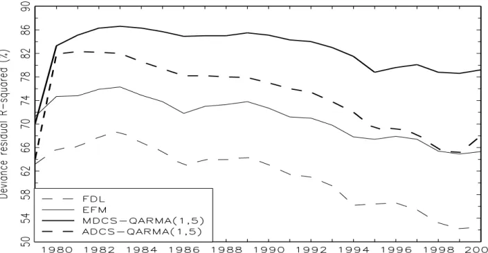
Both R-squared values are defined for each period t= 1, . . . , T. In Panels C and D of Table III we present the simple average over time of Pearson R-squared and deviance residual R-squared series. We show by bold numbers those well-specified models for which R&D is an exogenous variable. The results show that MDCS-QARMA(1,5) has the highest mean R-squared values, with respect to those models where R&D is exogenous. Due to the fact that simple average may be an inconsistent estimator and also misleading, we also present the evolution of Pearson R-squared and deviance R-squared in Figures 1 and 2, respectively, for period 1979 to 2000. In these figures, we present only those models for which R&D is exogenous. Figures 1 and 2 show that the superiority of MDCS-QARMA(1,5) is persistent over time, according to both R-squared metrics.
5. conclusions
In this paper we have introduced a new class of DCS models that allows us to estimate DCS time-series models for firm-level panels of patent count data. We have estimated several patent count panel data models for the extended panel data of patent applications used by
Blazsek and Escribano (2010, 2015). Different patent count data models have been estimated for a large panel of 4,476 US firms for period 1979 to 2000. We have considered three alternative estimation methods, MLE, QMLE and GMM, for count panel data models, and we conclude that the negative binomial QMLE is the most appropriate method. Exogeneity tests have indicated that R&D is exogenous for FDL, EFM, MDCS-QARMA(1,5) and ADCS-QARMA(1,5). For all other count panel data models R&D expenditure seems to be an endogenous variable, mainly due to omitted variables and the fact that the models are not dynamically complete. Hence, the conditional mean of patent count is misspecified. We have also used different R-squared metrics in order to compare the statistical performance of count panel data models, which suggest that the MDCS-QARMA(1,5) model is superior to other count panel data models considered.
REFERENCES
Blazsek, S., and A. Escribano(2010): “Knowledge Spillovers in U.S. Patents: A Dynamic Patent Intensity
Model with Secret Common Innovation Factors,”Journal of Econometrics, 159 (1), 14–32.
Blazsek, S., and A. Escribano (2015): “Patent Propensity, R&D and Market Competition: Dynamic
Spillovers of Innovation Leaders and Followers,”Journal of Econometrics, http://dx.doi.org/10.1016/j.jeconom.2015.10.005
Bloom, N., M. Schankerman, and J. Van Reenen(2013): “Identifying Technology Spillovers and Product
Market Rivalry,”Econometrica, 81 (4), 1347–1393.
Blundell, R., R. Griffith, and F. Windmeijer(2002): “Individual Effects and Dynamics in Count Data
Models,”Journal of Econometrics, 108 (1), 113–131.
Cameron, A. C., and P. K. Trivedi(1986): “Econometric Models Based on Count Data: Comparisons
and Applications of Some Estimators and Tests,”Journal of Applied Econometrics, 1 (1), 29–53.
Cameron, A. C., and P. K. Trivedi (2005): Microeconometrics Methods and Applications. Cambridge,
UK: Cambridge University Press.
Cameron, A. C., and F. A. G. Windmeijer (1996): “R-Squared Measures for Count Data Regression
Models with Applications to Health-Care Utilization,”Journal of Business & Economic Statistics, 14 (2), 209–220.
Davidson, R., and J. G. MacKinnon(2003): Econometric theory and methods. New York: Oxford Univer-sity Press.
Davis, R., W. Dunsmuir, and S. Streett (2003): “Observation-Driven Models for Poisson Counts,”
Biometrika, 90 (4), 777–790.
Davis, R., W. Dunsmuir, and S. Streett (2005): “Maximum Likelihood Estimation for an Observation
Driven Model for Poisson Counts,”Methodology & Computing in Applied Probability, 7 (2), 149–159.
Gourieroux, C., A. Monfort, and A. Trognon(1984a): “Pseudo Maximum Likelihood Methods:
The-ory,”Econometrica, 52 (3), 681–700.
Gourieroux, C., A. Monfort, and A. Trognon(1984b): “Pseudo Maximum Likelihood Methods:
Ap-plications to Poisson Models,”Econometrica, 52 (3), 701–720.
Griliches, Z.(1990): “Patent Statistics as Economic Indicators: A Survey,”Journal of Economic Literature,
28 (4), 1661–1707.
Hall, B., A. B. Jaffe, and M. Trajtenberg (2001): “The NBER Patent Citation Data File: Lessons,
Insights and Methodological Tools,” NBER Working Paper No. 8498.
Hansen, L. P.(1982): “Large Sample Properties of Generalized Method of Moments Estimators,”
Economet-rica, 50 (4), 1029–1054.
Harvey, A. C.(2013): Dynamic Models for Volatility and Heavy Tails. Cambridge, UK: Cambridge University
Press.
Hausman, J., B. Hall, and Z. Griliches(1984): “Econometric Models for Count Data with an Application
to the Patents-R&D Relationship,”Econometrica, 52 (4), 909–938.
Jaffe, A. B. (1986): “Technological Opportunity and Spillovers of R&D: Evidence from Firms’ Patents,
Profits, and Market Value,”American Economic Review, 76 (5), 984–1001.
Lanjouw, J. O., A. Pakes, and J. Putnam(1998): “How to Count Patents and Value Intellectual Property:
The Uses of Patent Renewal and Application Data,”The Journal of Industrial Economics, 46 (4), 405–432.
Lanjouw, J. O., and M. Schankerman(1999): “The Quality of Ideas: Measuring Innovation with Multiple
Indicators,” NBER Working Paper No. 7345.
Pakes, A.(1985): “On Patents, R&D, and the Stock Market Rate of Return,”Journal of Political Economy,
Trajtenberg, M.(1990): “A Penny for Your Quotes: Patent Citations and the Value of Innovations,”RAND
Journal of Economics, 21 (1), 172–187.
Wooldridge, J. M. (1997a): “Quasi-Likelihood Methods for Count Data,” in Handbook of Applied
Econo-metrics, Volume 2, ed. by M. H. Pesaran and P. Schmidt. Oxford: Blackwell, 352–406.
Wooldridge, J. M.(1997b): “Multiplicative Panel Data Models without the Strict Exogeneity Assumption,”
Econometric Theory, 13 (5), 667–678.
Wooldridge, J. M.(2002): Econometric Analysis of Cross Section and Panel Data. Cambridge, MA: The
MIT Press.
Wooldridge, J. M.(2005): “Simple Solutions to the Initial Conditions Problem in Dynamic, Nonlinear Panel
T ABLE I Mul tiplica tive Count P anel D a t a Models: Pooled Nega tiv e Binomial QMLE P arameter Estima tes P arameter FDL EFM MDCS-QMA(1) MDCS-QAR(1) MDCS-QARMA(1,1) MDCS-QARMA(1,5) µ0 − 1 . 8050 ∗∗∗ (0 . 1838) − 1 . 7523 ∗∗∗ (0 . 1542) − 1 . 1213 ∗∗∗ (0 . 0392) − 1 . 2426 ∗∗∗ (0 . 0309) − 1 . 2449 ∗∗∗ (0 . 0308) − 1 . 2505 ∗∗∗ (0 . 0304) γ1 t 0 . 0757 ∗∗∗ (0 . 0062) 0 . 0762 ∗∗∗ (0 . 0054) 0 . 0397 ∗∗∗ (0 . 0015) 0 . 0594 ∗∗∗ (0 . 0016) 0 . 0598 ∗∗∗ (0 . 0016) 0 . 0607 ∗∗∗ (0 . 0016) γ2 ( t × r dit ) − 0 . 0245 ∗∗∗ (0 . 0030) − 0 . 0194 ∗∗∗ (0 . 0025) − 0 . 0080 ∗∗∗ (0 . 0011) − 0 . 0079 ∗∗∗ (0 . 0011) − 0 . 0079 ∗∗∗ (0 . 0011) − 0 . 0079 ∗∗∗ (0 . 0011) γ3 D i 0 . 2133 ∗∗ (0 . 0910) 0 . 2476 ∗∗∗ (0 . 0731) 0 . 1835 ∗∗∗ (0 . 0314) 0 . 1583 ∗∗∗ (0 . 0279) 0 . 1577 ∗∗∗ (0 . 0278) 0 . 1599 ∗∗∗ (0 . 0275) γ4 zi 0 . 1168 ∗∗∗ (0 . 0344) 0 . 0996 ∗∗∗ (0 . 0273) 0 . 0653 ∗∗∗ (0 . 0075) 0 . 0572 ∗∗∗ (0 . 0054) 0 . 0568 ∗∗∗ (0 . 0054) 0 . 0559 ∗∗∗ (0 . 0052) γ5 ni 1 NA 0 . 0066 ∗∗∗ (0 . 0014) 0 . 0157 ∗∗∗ (0 . 0007) 0 . 0161 ∗∗∗ (0 . 0007) 0 . 0161 ∗∗∗ (0 . 0007) 0 . 0161 ∗∗∗ (0 . 0007) β0 r dit 0 . 8631 ∗∗∗ (0 . 0602) 0 . 7394 ∗∗∗ (0 . 0525) 0 . 3804 ∗∗∗ (0 . 0296) 0 . 3775 ∗∗∗ (0 . 0309) 0 . 3776 ∗∗∗ (0 . 0309) 0 . 3784 ∗∗∗ (0 . 0312) β1 r dit − 1 0 . 0502 ∗∗ (0 . 0218) 0 . 0136(0 . 0172) 0 . 0294(0 . 0228) 0 . 0247(0 . 0232) 0 . 0251(0 . 0234) 0 . 0241(0 . 0234) β2 r dit − 2 0 . 0492 ∗∗ (0 . 0227) 0 . 0383 ∗∗∗ (0 . 0127) 0 . 0372 ∗∗∗ (0 . 0097) 0 . 0353 ∗∗∗ (0 . 0094) 0 . 0356 ∗∗∗ (0 . 0095) 0 . 0369 ∗∗∗ (0 . 0094) β3 r dit − 3 0 . 0965 ∗∗∗ (0 . 0353) 0 . 0650 ∗∗∗ (0 . 0166) 0 . 0429 ∗∗∗ (0 . 0104) 0 . 0288 ∗∗∗ (0 . 0100) 0 . 0284 ∗∗∗ (0 . 0101) 0 . 0291 ∗∗∗ (0 . 0101) β4 r dit − 4 0 . 0165(0 . 0152) − 0 . 0061(0 . 0113) 0 . 0368 ∗∗∗ (0 . 0114) 0 . 0196 ∗(0 . 0106) 0 . 0189 ∗(0 . 0106) 0 . 0192 ∗(0 . 0107) β5 r dit − 5 0 . 0794 ∗∗∗ (0 . 0265) − 0 . 0245(0 . 0192) 0 . 0587 ∗∗∗ (0 . 0149) 0 . 0379 ∗∗∗ (0 . 0130) 0 . 0375 ∗∗∗ (0 . 0129) 0 . 0356 ∗∗∗ (0 . 0131) φ1 AR(1) NA 0 . 0113 ∗∗∗ (0 . 0003) NA 0 . 8682 ∗∗∗ (0 . 0119) 0 . 8721 ∗∗∗ (0 . 0134) 0 . 8992 ∗∗∗ (0 . 0238) θ0 uit NA NA 0 . 2390 ∗∗∗ (0 . 0026) 0 . 1968 ∗∗∗ (0 . 0025) 0 . 2000 ∗∗∗ (0 . 0025) 0 . 1999 ∗∗∗ (0 . 0025) θ1 uit − 1 NA NA 0 . 2008 ∗∗∗ (0 . 0027) NA − 0 . 0066 ∗∗∗ (0 . 0020) − 0 . 0079 ∗(0 . 0048) θ2 uit − 2 NA NA 0 . 1653 ∗∗∗ (0 . 0029) NA NA − 0 . 0069 ∗ (0 . 0042) θ3 uit − 3 NA NA 0 . 1342 ∗∗∗ (0 . 0028) NA NA − 0 . 0064 ∗(0 . 0036) θ4 uit − 4 NA NA 0 . 1037 ∗∗∗ (0 . 0028) NA NA − 0 . 0049(0 . 0031) θ5 uit − 5 NA NA 0 . 0320 ∗∗ (0 . 0134) NA NA − 0 . 0089 ∗∗∗ (0 . 0027) δ 0 . 8008 ∗∗∗ (0 . 1401) 0 . 3111 ∗∗∗ (0 . 0822) 0 . 3120 ∗∗∗ (0 . 0549) 0 . 2593 ∗∗∗ (0 . 0386) 0 . 2595 ∗∗∗ (0 . 0386) 0 . 2587 ∗∗∗ (0 . 0388) Notes : Robust standard errors are rep orted in paren theses. *, ** and *** indicate significance at the 10%, 5% and 1% lev els, resp ectiv ely .
T ABLE II Additive Count P anel D a t a Models: Pooled N ega tive Binomial QMLE P arameter Estim a tes P arameter LFM ADCS-QMA(1) ADCS-QAR(1) ADCS-QARMA(1,1) ADCS-QARMA(1,5) µ0 − 2 . 5382 ∗∗∗ (0 . 0421) − 2 . 2299 ∗∗∗ (0 . 0851) − 2 . 2377 ∗∗∗ (0 . 0848) − 2 . 2458 ∗∗∗ (0 . 0905) − 2 . 2519 ∗∗∗ (0 . 0907) γ1 t 0 . 0394 ∗∗∗ (0 . 0018) 0 . 0323 ∗∗∗ (0 . 0030) 0 . 0301 ∗∗∗ (0 . 0030) 0 . 0302 ∗∗∗ (0 . 0030) 0 . 0296 ∗∗∗ (0 . 0031) γ2 ( t × r dit ) − 0 . 0160 ∗∗∗ (0 . 0006) − 0 . 0076 ∗∗∗ (0 . 0021) − 0 . 0072 ∗∗∗ (0 . 0021) − 0 . 0071 ∗∗∗ (0 . 0021) − 0 . 0069 ∗∗∗ (0 . 0021) γ3 D i 0 . 3545 ∗∗∗ (0 . 0146) 0 . 3209 ∗∗∗ (0 . 0493) 0 . 3232 ∗∗∗ (0 . 0492) 0 . 3248 ∗∗∗ (0 . 0496) 0 . 3301 ∗∗∗ (0 . 0497) γ4 zi 0 . 0940 ∗∗∗ (0 . 0037) 0 . 1178 ∗∗∗ (0 . 0153) 0 . 1195 ∗∗∗ (0 . 0150) 0 . 1203 ∗∗∗ (0 . 0152) 0 . 1224 ∗∗∗ (0 . 0151) γ5 ni 1 0 . 0059 ∗∗∗ (0 . 0003) 0 . 0092 ∗∗∗ (0 . 0009) 0 . 0091 ∗∗∗ (0 . 0009) 0 . 0090 ∗∗∗ (0 . 0009) 0 . 0089 ∗∗∗ (0 . 0009) β0 r dit 1 . 0647 ∗∗∗ (0 . 0148) 0 . 6468 ∗∗∗ (0 . 0563) 0 . 6461 ∗∗∗ (0 . 0569) 0 . 6442 ∗∗∗ (0 . 0568) 0 . 6430 ∗∗∗ (0 . 0571) β1 r dit − 1 − 0 . 3582 ∗∗∗ (0 . 0104) 0 . 1192 ∗∗∗ (0 . 0366) 0 . 1164 ∗∗∗ (0 . 0364) 0 . 1200 ∗∗∗ (0 . 0369) 0 . 1178 ∗∗∗ (0 . 0373) β2 r dit − 2 − 0 . 0834 ∗∗∗ (0 . 0079) 0 . 0590 ∗∗∗ (0 . 0151) 0 . 0589 ∗∗∗ (0 . 0156) 0 . 0578 ∗∗∗ (0 . 0151) 0 . 0573 ∗∗∗ (0 . 0151) β3 r dit − 3 − 0 . 0206 ∗∗ (0 . 0089) 0 . 0369 ∗∗ (0 . 0177) 0 . 0436 ∗∗ (0 . 0174) 0 . 0430 ∗∗ (0 . 0182) 0 . 0444 ∗∗ (0 . 0176) β4 r dit − 4 − 0 . 0286 ∗∗∗ (0 . 0109) 0 . 0101(0 . 0099) 0 . 0053(0 . 0097) 0 . 0045(0 . 0097) 0 . 0050(0 . 0098) β5 r dit − 5 − 0 . 0373 ∗∗∗ (0 . 0075) 0 . 0749 ∗∗∗ (0 . 0209) 0 . 0783 ∗∗∗ (0 . 0208) 0 . 0790 ∗∗∗ (0 . 0207) 0 . 0782 ∗∗∗ (0 . 0207) φ1 AR(1) 0 . 9215 ∗∗∗ (0 . 0254) NA 0 . 5746 ∗∗∗ (0 . 0221) 0 . 6159 ∗∗∗ (0 . 0404) 0 . 8328 ∗∗∗ (0 . 0478) θ0 uit NA 0 . 3690 ∗∗∗ (0 . 0065) 0 . 3292 ∗∗∗ (0 . 0065) 0 . 3567 ∗∗∗ (0 . 0083) 0 . 3586 ∗∗∗ (0 . 0107) θ1 uit − 1 NA 0 . 1877 ∗∗∗ (0 . 0032) NA − 0 . 0569 ∗∗∗ (0 . 0100) − 0 . 1180 ∗∗∗ (0 . 0094) θ2 uit − 2 NA 0 . 0926 ∗∗∗ (0 . 0024) NA NA − 0 . 0606 ∗∗∗ (0 . 0043) θ3 uit − 3 NA 0 . 0536 ∗∗∗ (0 . 0021) NA NA − 0 . 0238 ∗∗∗ (0 . 0025) θ4 uit − 4 NA 0 . 0327 ∗∗∗ (0 . 0020) NA NA − 0 . 0091 ∗∗∗ (0 . 0021) θ5 uit − 5 NA 0 . 0130 ∗∗∗ (0 . 0017) NA NA − 0 . 0128 ∗∗∗ (0 . 0020) δ 0 . 0476 ∗∗∗ (0 . 0069) 0 . 5644 ∗∗∗ (0 . 1277) 0 . 5641 ∗∗∗ (0 . 1282) 0 . 5637 ∗∗∗ (0 . 1282) 0 . 5631 ∗∗∗ (0 . 1281) Notes : Robust standard errors are rep orted in paren theses. ** and *** ind ic ate significance at the 5% and 1% lev els, re sp ectiv ely .
T ABLE II I Ex ogeneity Tests and Model Perf ormance Metrics P anel A. T est of exogeneit y of R&D for m ultiplicativ e mo dels P arameter FDL EFM MDCS-QMA(1) MDCS-QAR(1) MDCS-QARMA(1,1) MDCS-QARMA(1,5) ρ1 0 . 0012(0 . 0098) − 0 . 0053(0 . 0069) − 0 . 0016(0 . 0047) 0 . 0018(0 . 0047) 0 . 0017(0 . 0047) 0 . 0018(0 . 0585) ρ2 − 0 . 2337(0 . 1774) − 0 . 1940(0 . 1240) − 0 . 2284 ∗∗∗ (0 . 0882) − 0 . 2590 ∗∗∗ (0 . 0915) − 0 . 2582 ∗∗∗ (0 . 0910) − 0 . 2582(1 . 2093) T est result R&D exogenous R&D exogenous R&D endogenous R&D endogenous R&D endogenous R&D exogenous P anel B . T est of exogeneit y of R&D for additiv e mo dels P arameter LFM ADCS-QMA(1) ADCS-QAR(1) ADCS-QARMA(1,1) ADCS-QARMA(1,5) ρ1 0 . 0054 ∗∗ (0 . 0027) − 0 . 0013(0 . 0104) − 0 . 0011(0 . 0105) − 0 . 0012(0 . 0104) − 0 . 0013(0 . 0842) ρ2 − 0 . 7617 ∗∗∗ (0 . 0492) − 0 . 5817 ∗∗∗ (0 . 1537) − 0 . 5968 ∗∗∗ (0 . 1542) − 0 . 5956 ∗∗∗ (0 . 1546) − 0 . 5932(1 . 7437) T est result R&D endogenous R&D endogenous R&D end oge n ous R&D endogenous R&D exogenous P anel C . P erformance metrics for m ultiplicativ e mo dels Mean R 2 FDL EFM MDCS-QMA(1) M DCS-QAR(1) MDCS-QARMA(1,1) MDCS-QARMA(1,5) R 2 P, NB2 84 . 90 % 94 . 53 % 98 . 67% 98 . 70% 98 . 70% 98 . 69 % R 2 DEV , NB2(ML) 61 . 21 % 71 . 10 % 81 . 07% 82 . 57% 82 . 57% 82 . 59 % P anel D. P erformance metrics for additiv e mo dels Mean R 2 LFM ADCS-QMA(1) ADCS-QAR(1) ADCS-QARMA(1,1) ADCS-QARMA(1,5) R 2 P, NB2 97 . 73% 96 . 57% 96 . 54% 96 . 53% 96 . 52 % R 2 DEV , NB2(ML) 89 . 92% 74 . 63% 74 . 71% 74 . 72% 74 . 74 % Notes : W e study whether R&D is exogenous b y using the W o oldridge (1997a, 2002) test. Significan t ρ1 or ρ2 indicate endogeneit y of curren t R&D exp enditure. Robust stand ard err ors are rep orted in paren theses. ** and *** indicate significance at the 5% and 1% lev els, resp ectiv ely . P earson R-squared and deviance residual R-squared v alues are computed according to Cameron and Windmeijer (1996) and applied to pan e l data. Bold R-squared v alues indicate that R&D is exoge n ous v ariable for the corresp onding mo del.