DAGViz: A DAG Visualization Tool for Analyzing Task Parallel Programs (DAGViz: DAG )

(1)

修士論文

DAGViz: A DAG Visualization Tool for

Analyzing Task Parallel Programs

(DAGViz:

タスク並列計算の性能解析のた

めの

DAG

可視化ツール)

平成

27 年

2 月

5 日提出

指導教員

田浦健次朗

准教授

電子情報学専攻

48-136431 Huynh Ngoc An

(2)

Abstract

Task parallel programming model has been considered as a promising mean that brings parallel programming to larger audience thanks to its high programmability. In task parallel program-ming, programmers just need to specify tasks that can be executed in parallel then these tasks would be distributed to available processor cores and executed in parallel dynamically by the runtime system. However, this dynamic characteristics of task parallelism hides all execution mechanisms of a task parallel application from programmers, which makes it difficult for them to understand suboptimal performance of their application. We have developed tools to cap-ture relevant data during the execution of a task parallel application as a directed acyclic graph (DAG) of sequential code sections of application code. then visualize captured data. Our visual-izer displays DAG in a hierarchical way that helps users conceive DAG structure at various levels of detail. It also provides multiple views for a single DAG and supports coordination between them, which has yielded interesting information as we case-study the applications in Barcelona OpenMP Task Suite (BOTS). Specifically, the tool could pinpoint relevent code sections that causes low parallelism time periods of interest. Moreover, this approach is prospective in the way that we can visually compare two isomorphic DAGs generated by the same application running on different environments which we intend to do in future work. This comparison is expected to expose differences between task parallel runtime systems and exhibit insights useful for developing scheduling algorithm.

(3)

List of Figures

1.1 A task parallelfibonacci program . . . 5

1.2 Common API code gets translated intoOpenMP,Cilk and Intel TBB codes au-tomatically . . . 7

1.3 DAG of fib(3) execution . . . 9

1.4 All node kinds of DAG Recorder (or PIDAG) . . . 9

1.5 DAG Recorder’s node . . . 10

1.6 An example of task parallel computational DAG . . . 10

1.7 Node info structure . . . 11

1.8 BOTS’s scalability . . . 12

1.9 Compare six task parallel systems running Sort . . . 13

1.10 Breakdown graphs of Sort on 1, 16, 32, 64 core(s) . . . 14

1.11 Breakdown graphs of Sort based on MassiveThreads, Intel CilkPlus, OpenMP, Intel TBB . . . 15

1.12 Sort’s scalability and breakdown graphs . . . 16

1.13 Sort’s parallelism profile at 64-core execution byMassiveThreads . . . 16

1.14 Strassen’s scalability and breakdown graphs . . . 17

1.15 Strassen’s parallelism profile at 64-core execution byMassiveThreads . . . 17

3.1 P-D-V design . . . 22

3.2 Flattened DAG Recorder’s nodes in PIDAG of fib(3) program . . . 23

3.3 PIDAG’s node . . . 23

3.4 Node’s linking variables . . . 25

3.5 Hierarchical layout model . . . 26

3.6 DAG traversal model . . . 27

3.7 Node’s coordinate variables . . . 28

3.8 Section and Task’s topology . . . 29

3.9 Four kinds of view . . . 29

3.10 Scale down . . . 30

3.11 Sort’s parallelism profile at depth 1 . . . 31

3.14 Animation’s rate . . . 33

3.15 Rate of alpha for fading out/in . . . 33

4.1 Alignment . . . 36 4.2 FFT . . . 36 4.3 Fib . . . 37 4.4 Floorplan . . . 37 4.5 Health . . . 37 4.6 NQueens . . . 37 4.7 Sort . . . 38 4.8 SparseLU . . . 38

(6)

4.9 Strassen . . . 38

4.10 UTS . . . 38

5.1 dr overhead of mth on 64 workers . . . 39

5.2 DAG size’s ranges . . . 40

A.1 P data structure . . . 49

A.2 D data structure . . . 50

A.3 V data structure . . . 51

A.4 DAGViz’s node . . . 52

B.1 DAG with round nodes’s layout algo phase 1 . . . 54

B.2 DAG with round nodes’s layout algo phase 2 . . . 55

B.3 DAG with long nodes’s layout algo phase 1 . . . 56

B.4 DAG with long nodes’s layout algo phase 2 . . . 57

(7)

List of Tables

4.1 Environment . . . 35 4.2 Benchmark applications . . . 35 4.3 Summary of benchmarks settings. They are all the applications in Barcelona

OpenMP Task Suites. . . 36 4.4 Experiment results . . . 36

(8)

Chapter 1

Introduction

Due to some physical limitations such as heat dissipation, the development of computer hard-ware has changed from increasing clock speed of a single-core CPU to increasing the number of cores integrated in a multi-core CPU for more than a decade. There are more and more cores which are integrated in a computer’s CPU, from 4 to 8 ones in a commodity PC up to 64 ones in a high performance computing server. Along with that change in hardware, another programming model is needed to create software that can run on the new hardware architecture which is usually called as parallel programs. A parallel program consists of multiple computing threads which run at the same time, and each thread resides on one separate core.

A traditional approach to creating parallel programs on shared memory systems is that the programmer demands thread creation one by one and assign work for each thread by themself. Given that a computer has 64 cores, a programmer who wants to use all that computer’s processing power has to write code to create 64 threads and divide work to 64 portions in his program. POSIX Threads [1] is a library that provides this kind of programming model. However, this kind of programming style makes programmers exhausted of thread managing work rather than focusing their strength on developing the program’s algorithm. Moreover, recent surge of Many Integrated Core (MIC) architecture developed by Intel has put a new prospect on shared memory parallel programs which may now need to manage up to several hundred simultaneously running threads. There is a need for a parallel programming model that releases programmers from low-level detailed concerns so that they can take care better of higher-level things and parallel programming can reach to more programmers who are usually ignorant of low-level system and hardware knowledge.

Task parallel programming models help solving this problem. It has a very high programma-bility, meaning easy to use for programmers to create parallel program. In the next section, we talk about some task parallel programming models and the common API that we created to unify their code.

1.1 Task Parallel Programming Models

In task parallelism, programmers just need to create as many tasks as possible, each task is an execution of some function, and a task can create other tasks recursively. The other burdens in parallel execution such as thread management, task stealing/migration, load balancing are taken care by the runtime system. Therefore, the runtime system plays an important role in the performance of a task parallel program.

Figure 1.1 illustrates a pseudo-code example of thefibonacci program written in task paral-lelism. This example exhibits two main interfaces of a task parallel programming model. They are an interface to create a task (Create Task) and another interface to wait for tasks that

have been created (Wait Tasks). This simple example has demonstrated task parallelism’s

(9)

1 intfib(intn){

2 if(n<2)

3 return1;

4 else{

5 intx, y;

6 x = Create Task( fib(n−1) );

7 y = Create Task( fib(n−2) );

8 _{Wait Tasks}();

9 returnx+y;

10 } 11 }

Figure 1.1. A task parallelfibonacci program

creation primitives so that their program becomes a parallel one which can run on any (shared-memory) parallel hardware environment, task parallelism is easy to use and particularly fit with divide-and-conquer algorithms. Thus, it is promising to bring the tricky parallel programming technique to a wider adoption among general programmers.

1.1.1 A Common Interface for All Six Task Parallel Systems

There are various task parallel programming models existing such as OpenMP [2], Cilk [3]

(Intel CilkPlus[4]),Intel TBB[5],QThreads[6],MassiveThreads[7] [8], andNanos++[9]. They

may be a language (OpenMP, Cilk, Intel CilkPlus) or just a library (Intel TBB, QThreads,

MassiveThreads, Nanos++) that provides interface functions to access the task parallel

run-times. Although each model has distinct diﬀerences in its API, they all support the two basic interfaces showed in Figure 1.1, Create Task and Wait Tasks.

OpenMP model defines an additional set of compiler directives to a language (C, C++,

Fortran) in order to provide task parallelism for that language. In OpenMP, Create Task

manifests as a directive pragma beginning with “#pragma omp task”, and Wait Tasks

mani-fests as a pragma of “#pragma omp taskwait” (Figure 1.2b). Cilklanguage is formed by adding some additional keywords to the C language to support task parallelism. These keywords include

“spawn” which is equivalent toCreate Task, and “sync” which is equivalent toWait Tasks

(Figure 1.2c).

On the other hand, Intel TBB model is a C++ library providing task group class in the

tbb namespace. task group’s run function corresponds to the Create Task primitive and

task group’s wait function corresponds to the Wait Tasks primitive (Figure 1.2d). We have

implemented another task group version that interfaces with the other 3 task parallel libraries

QThreads,MassiveThreadsand modelnanox. Thus, writing code for these libraries is as much

similar as writing code forIntel TBB.

In order to evaluate all these six task parallel systems together with ease we have created a common application program interface (API) covering all common grounds as well as distinct diﬀerences between them. Another primitive ofMake Task Group(mk task group) is added

to represent Intel TBB model’s task group declaration, which does not exist in OpenMP and

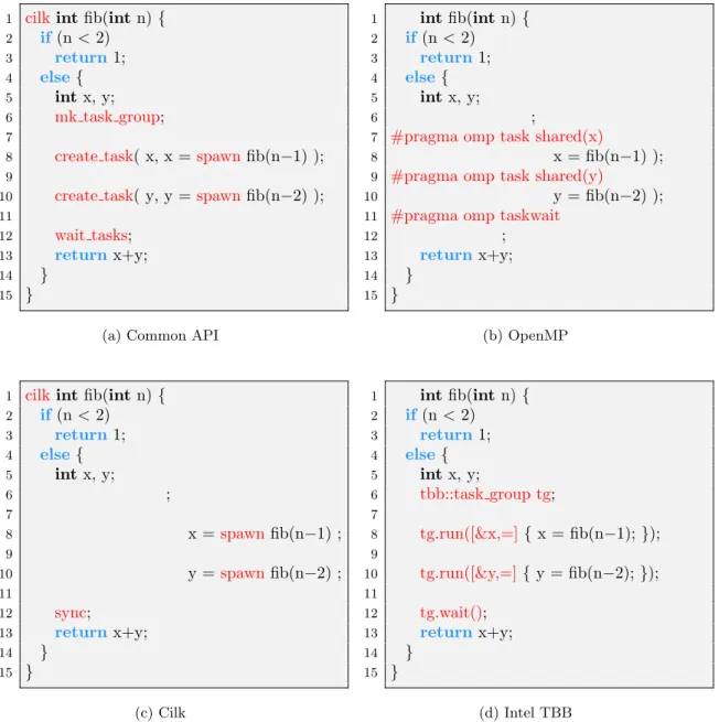
Cilk models. We built a macro wrapper that translates code based on this common API into six individual executables corresponding to the six systems in compile time. An example of the common API used in fibonacci program is showed in Figure 1.2a. Figure 1.2 gathers 4 versions of the fib program based on the common API, OpenMP, Cilk and Intel TBB models. In addition, it also illustrates how a common API code gets transformed into these models. In general, the method is that a common syntax between the common API and the target model is replaced by the target model’s semantics, and a syntax that exists in the common API but does not exist in the target model will get deleted.

(10)

This common API eases the process of porting a program’s code into all six runtime sys-tems. We now just need to write code once and get it compiled to six individual executables corresponding to the six systems.

1.1.2 Critical Role of Task Parallel Runtimes

In task parallelism, the burden on programmers has been released, but that on the runtime sys-tem has been piled up instead. The runtime syssys-tem’s job in task parallelism can be generalized in following 3 parts:

• interfacing with the underlying hardware.

• managing all created tasks and their parent-child relationships.

• delivering tasks to free doing-nothing threads so that the work is balanced between avail-able threads.

All these parts are done dynamically at runtime. A common approach to the first part is that the runtime system would initiate a certain number of concurrent threads at the beginning of the program’s execution, which corresponds to the number of available processor cores in the underlying hardware, each thread is bound to a single separate processor core, and usually referred to asworker threads or simply workers. For the second part, each worker maintains a work queue of its own, and every task is stored in the work queue of the worker on which it is created. A worker executes tasks in its work queue one by one until it runs out of tasks (its work queue gets empty). At that time, it will go to steal work from other workers who have tasks waiting in their queues. The stealing mechanism is that the free worker chooses a victim worker randomly, then goes to see if the victim worker’s work queue has any task available, if there is, it will migrate that task to its thread and execute it. If there is no task remained in the victim’s queue, it will choose another victim and go stealing again, and continue with other victims continuously until it can steal a task. This load balancing mechanism is called

work stealing [10]. Work stealing is one of the mechanisms that a task parallel runtime uses to

accomplish its third part.

When a worker creates a new task, it has two choices to proceed, one is to pause the current task and switch to executing the new task. The other is opposite, the worker pushes the new task into its work queue and continue executing the current task. These approaches are usually referred to as work-first, and help-first respectively [11]. Work-first’s execution order is similar to that of a serial execution. Therefore, it is expected to maintain the best data locality and hence perform better than help-first. On the other hand, help-first tends to spawn as many tasks as possible, exhibiting better parallelism for the scheduler to feed available workers. There is no absolute answer to the question of which one, work-first or help-first, is better yet. Because which one performs better may also depends on the computation model of the program’s algorithm and possibly the number of underlying available workers. As we know,

OpenMP, Intel TBB and QThreads adopt help-first policy in their schedulers. Intel CilkPlus

and MassiveThreadsadoptwork-first.

Apparently the third part doing load balancing is the most important part of a task parallel runtime system which decides its implementation’s quality. The better it is implemented the better performance the runtime can deliver when executing task parallel programs. However, the fact that load balancing is done dynamically at runtime and automatically by the runtime system leads to another fact that a great deal of performance formation is out of the programmer’s control. The same task parallel program, meaning the same algorithm, executed by diﬀerent task parallel runtimes could possibly present significantly diﬀerent degrees of performance. And the programmer has no clue of why it happens because all mechanisms inside the runtimes are hidden from him.

Solving this problem is critical to the development of task parallel programming models. As an attempt to attack it, we have built a tool that records relevant events during the execution of

(11)

1 cilkintfib(intn){ 2 if(n<2) 3 return1; 4 else { 5 intx, y; 6 mk task group; 7

8 create task( x, x = spawnfib(n−1) );

9

10 create task( y, y = spawnfib(n−2) );

11

12 wait tasks; 13 returnx+y;

14 } 15 }

(a) Common API

2 if(n<2)

3 return1;

4 else{

5 intx, y;

6 ;

7 #pragma omp task shared(x)

8 x = fib(n−1) );

9 #pragma omp task shared(y)

10 y = fib(n−2) );

11 #pragma omp taskwait

12 ;

13 returnx+y;

14 } 15 }

(b) OpenMP

1 cilkintfib(intn){

2 if(n<2) 3 return1; 4 else { 5 intx, y; 6 ; 7 8 x =spawn fib(n−1) ; 9 10 y =spawn fib(n−2) ; 11 12 sync; 13 returnx+y; 14 } 15 } (c) Cilk

2 if(n<2) 3 return1; 4 else{ 5 intx, y; 6 tbb::task group tg; 7 8 tg.run([&x,=]{x = fib(n−1); }); 9 10 tg.run([&y,=]{y = fib(n−2);}); 11 12 tg.wait(); 13 returnx+y; 14 } 15 } (d) Intel TBB

Figure 1.2. Common API code gets translated into OpenMP,Cilk and Intel TBB codes auto-matically

(12)

a task parallel program so that we can analyze the performance of the execution port-mortemly. It is called DAG Recorder and built upon the common API so it can work with all six task

parallel systems.

1.2 DAG Recorder

DAG Recorder is a performance measurement module that runs along with an execution

of a task parallel program and records all relevant performance events occurring during that execution then stores them in a format of a directed acyclic graph (DAG) of nodes and edges.

DAG Recorder is built inside the common API, so programs written in this common API

can use DAG Recorder immediately with a minimal involvement of the programmer. This

is following three main API functions that the programmer need to remember:

• dr start()

• dr stop()

• dr dump()

The programmer usesdr start()to orderDAG Recorderto start its measurement,dr stop()

to stop DAG Recorder’s measurement and dr dump() to make DAG Recorder dump its

measurement data currently stored in memory out to files. Besides, DAG Recorder also

de-fines several environment variables for programmers to tweak its behaviors. DAG Recorder’s

usage is just that simple. We are going to describe DAG Recorder’s three aspects of what

kind of DAG that it records, how it does the measurement, and what kind of information it can provide.

1.2.1 DAG Structure

A computational DAG of a task parallel program consists of a set of nodes and a set of edges. Each node represents a sequential code segment in the application-level code that does not contain any task parallel primitive. Edges are the manifests of those task parallel primitives, they represent the task-parallelism-style relationships between nodes. These relationships are:

• parent-child (spawning) relationship

• continuation relationship

• synchronizing relationship

For example, two contiguous code segments separated by a Create Task primitive in

the application’s code would have continuation relationship between them. The code segment preceding Create Task and the first code segment of the function assigned to the task

cre-ated by Create Task would have spawning relationship. The last code segments of all tasks

(or functions) synchronized by aWait Tasks primitive and the code segment preceding that Wait Tasks primitive would bear asynchronizing relationship with the code segment

follow-ing thatWait Tasksprimitive. There are possibly two or more nodes that havesynchronizing

edges pointing to a single node of the code segment following Wait Tasks depending on how

many tasks that Wait Taskssynchronizes.

DAG Recorder classifies nodes into 3 node kinds based on the task parallel primitives

that end their code segments. A code segment ended by Create Task is represented by a

create node. A code segment ended by Wait Tasks is represented by a wait node. The last

code segment of a task (function) is called an end node. Based on this naming, a small DAG

of afib(3) program is showed in Figure 1.3.

Actually the DAG’s structure is hierarchical. Three kinds of create, wait and end are just terminal nodes that do not contain any sub-graph inside them. There are two other kinds of

(13)

Figure 1.3. DAG of fib(3) execution

Figure 1.4. All node kinds of DAG Recorder (or PIDAG)

non-terminal nodes which aresectionandtask. They are collective nodes containing sub-graphs of terminal or other collective nodes inside. All these 5 kinds of nodes are shown in Figure 1.4. A tasknode corresponds to a task entity in the runtime system. It can contain none, one or multiplesection nodes before ending by an endnode. A section node contains one or multiple

createand sectionnodes before ending by a waitnode. The purpose of sectionkind is to mark

all tasks that will get synchronized by a Wait Tasks primitive. All tasks created by child

createnodes in asectionnode are synchronized by the last childwaitnode of thatsectionnode.

Figure 1.5 shows the member variables of aDAG Recorder’s node’s structure: infois a child

structure that holds all performance information related to the code segment that the node represents, next is a pointer to the next node in the list of all child nodes of its parent, if the node is of createkind child pointer will point to the task node that it creates, if the node is a collective node of kind taskorsection subgraphs list will contain all its child nodes.

1.2.2 Methodology

In order to capture the DAG structure as described in the previous sub-section,DAG Recorder

needs to instrument measurement code at following seven positions:

• EnterCreateTask: right before entering theCreate Task primitive

• LeaveCreateTask: right after leaving the Create Task primitive

• EnterWaitTasks: right before entering the Wait Tasks primitive

• LeaveWaitTasks: right after leaving theWait Tasks primitive

• StartTask: right before starting a new task

• EndTask: right before ending a task

• MakeSection: to mark the start of a newsection

Let’s consider the above items also as the code that need to be inserted at corresponding positions. DAG Recorder has modified the process through which a common API primitive

is translated into a specific task parallel API so that it puts these code at appropriate posi-tions. Inside Create Task, DAG Recorder puts EnterCreateTask as near the upper code

as possible,LeaveCreateTask as near the lower code as possible, StartTask right before execut-ing the task function andEndTask right after the task function finishes. InsideWait Tasks,

(14)

1 struct dr dag node{

2 dr dag node infoinfo;

3 structdr dag node ∗next;

4 union{

5 struct dr dag node∗child;

6 dr dag node listsubgraphs[1];

7 } 8 }

Figure 1.5. DAG Recorder’s node

A() { for(i=0;i<2;i++) { task_group tg; tg.run(B); tg.run(C); D(); tg.wait(); } } D() { task_group tg; tg.run(E); tg.wait(); } E C CreateTask WaitTasks EndTask B E C B CreateCont Create WaitCont Wait D() D()

Figure 1.6. An example of task parallel computational DAG

DAG RecorderputsEnterWaitTasks as near the upper code as possible andLeaveWaitTasks

as near the lower code as possible. Inside Make Task Group, DAG Recorder sets a flag

to remember to create a new sectionto enclose all following nodes that is other than endnode and await node would end thatsection.

StartTask, LeaveCreateTask and LeaveWaitTasks are positions where an interval (a node)

begins, so DAG Recorder records necessary information such as file name, line number,

time, worker number, cpu number in order to later combine with an end interval information to construct a full node. End interval information is recorded atEndTask,EnterCreateTask, and

EnterWaitTasks.

Figure 1.6 demonstrates the collective task node kind and how a section marks eﬀective

tasks to be synchronized by await. White nodes with one character inside are oftaskkind. The transition to a new sectionis indicated by the task group tg; declaration.

DAG Recorder has an useful feature of on-the-fly contraction that it can contract

un-interesting subgraphs into only one node. An unun-interesting subgraph is a subgraph that was executed wholly on a single worker. There was no work stealing, task migration happenning in that subgraph. Such kind of subgraphs is not interesting from the perspective of task parallel performance analysis. Contracting them does not aﬀect our performance analysis potential, and also helps reduce a considerable number of nodes in the DAG which is helpful for the vi-sualizer that visualizes the DAG. When atask or asectionis contracted, the statistical data of its child nodes are aggregated into its dr dag node info structure (Figure 1.7). For a section,

DAG Recorder also includes statistical data of alltask nodes created by thesection’s create

nodes.

1.2.3 Capability

DAG Recorderobserves all execution intervals of a task parallel program and manifests these

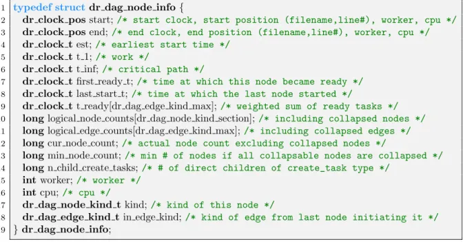
intervals as nodes in the DAG. Each node of the DAG holds adr dag node info structure (Fig-ure 1.7) that stores relevant performance data of the interval’s execution. In short, currently

(15)

1 typedef structdr dag node info{

2 dr clock posstart;/* start clock, start position (filename,line#), worker, cpu */

3 dr clock posend;/* end clock, end position (filename,line#), worker, cpu */

4 dr clock test;/* earliest start time */

5 dr clock tt 1;/* work */

6 dr clock tt inf;/* critical path */

7 dr clock tfirst ready t;/* time at which this node became ready */

8 dr clock tlast start t;/* time at which the last node started */

9 dr clock tt ready[dr dag edge kind max];/* weighted sum of ready tasks */

10 longlogical node counts[dr dag node kind section]; /* including collapsed nodes */

11 longlogical edge counts[dr dag edge kind max];/* including collapsed edges */

12 longcur node count;/* actual node count excluding collapsed nodes */

13 longmin node count;/* min # of nodes if all collapsable nodes are collapsed */

14 longn child create tasks;/* # of direct children of create_task type */

15 intworker;/* worker */

16 intcpu;/* cpu */

17 dr dag node kind tkind;/* kind of this node */

18 dr dag edge kind tin edge kind;/* kind of edge from last node initiating it */

19 } dr dag node info;

Figure 1.7. Node info structure

DAG Recorder records time metrics and source code positions. Source code position

infor-mation is critical for tracing back to the responsible application-level code blocks that occur the time metrics quantities. The recording source code positions also shows the superiority of

DAG Recorder’s instrumentation approach. By instrumenting measurement code into

ap-plication code, DAG Recorder can avoid the painful process of extracting application-level

information from binary executables that is needed by the sampling measurement approach. In general,DAG Recorder can attributing time metrics back up to application-level code which

is useful for programmers to analyze their application’s performance.

The information that a node can provide about the performance of the interval it represents can be described shortly below:

• start and end positions (filename, line number) of the code segment.

• est (earliest start time): this is the start time of the node if it is single, or the start time of its head child node if it is collective.

• t 1: work time of the node or collective work time of its child nodes.

• t inf: critical path of its subgraph or just equalst 1 if the node is single.

• first ready t: time at which the last of its dependent nodes finishes, making it ready to

execute.

• last start t: time at which the last of its child nodes gets started, or just equals est if the

node is single.

• worker: the worker on which this node was executed on

• cpu: the core number on which this node was executed on

We are next going to discuss some useful information based on the DAG thatDAG Recorder

records such as work, critical path, time series of actual and available parallelism, steal history.

Work

Based on the DAG we can know when a worker is working on the application’s code and when it is not. The time that a worker is working on application code is considered aswork timeor simplywork. The time that it executes other code such as runtime system’s code and the time it is idle are not work time. This non-work execution time of a worker can be classified into two

(16)

10 20 30 40 50 60 10 20 30 40 50 60 speedup workers BOTS mth ideal alignment fft fib floorplan health nqueens sort sparselu strassen uts

Figure 1.8. BOTS’s scalability

categories of delay and nowork (idleness). By subtracting the end and start time of a node, we can calculate its work, and summarizing them of all nodes in a DAG would give us the total work of the execution. The time a worker moves from aEnterCreateTaskinstrumentation point to its consecutive StartTask point (for work-first based scheduler) is considered asdelay time. It is also delay for the intervals betweenEnterCreateTask and LeaveCreateTask (for help-first based scheduler). The time that a worker is not executing anything isnowork.

The total elapsed time of all workers in an execution equals to the multiplication of the execution time and the number of processor cores on which the execution occurred. We refer to this kind of time quantity asworker timewith the meaning that it is the time an application uses workers. This is analogous to the definition of “CPU time” which is commonly defined the time that a process uses computer CPU.

Based on the DAG, we can break down worker time of an execution into 3 categories of

work,delayand nowork.

We have run DAG Recorder with all ten applications in the Barcelona OpenMP Task

Suite (BOTS) benchmark suite [12] and aquired the DAG of every execution. Experiment environment and parameters for each benchmark are described in Chapter 4’s Table 4.1 and Table 4.3.

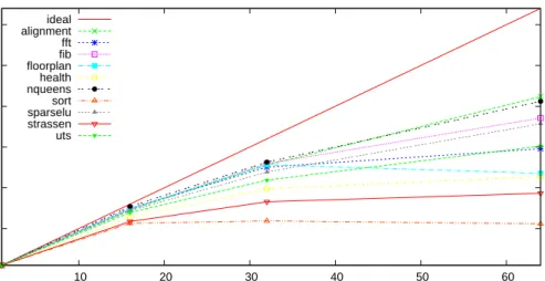
Based on simple execution times of the experiments we can draw a scalability graph of all

MassiveThreadsmodel based applications in Figure 1.8.

The experiments were conducted on the same machine with the same compiler. Thus, there are still only 3 experiment parameters varying, they are the application (app), the number of cores (ppn) and the task parallel model (type) in use. A combination of specific app-ppn

-type indicates a single experiment execution (or a single DAG) of the type model-based app

application onppncores. In Figure 1.8, thetype parameter remains the same asMassiveThreads, only app and ppn vary in the graph. On the other hand, in Figure 1.9 the app parameter remains the same as Sort,ppn and type vary. One more diﬀerent point is that Figure 1.8 plots the speedup values which are the ratios of the execution time ofppn= 1 over other ppns, while as Figure 1.9 plots the worker times of the executions.

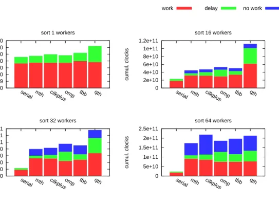
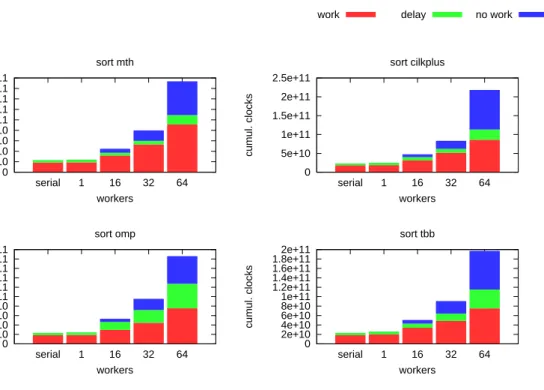
By fixing ppn parameter, the graph in Figure 1.9 can get split into 4 graphs in Figure 1.10. Moreover, in Figure 1.10 each bar which represents an execution is divided to 3 parts of 3 colors corresponding towork,delay andnowork components of the execution’s worker time.

(17)

0 10 20 30 40 50 60 70 80 90 1 16 32 64

workers $\times$ time (sec)

workers sort serial mth cilkplus omp tbb qth

Figure 1.9. Compare six task parallel systems running Sort

4 graphs corresponding to 4 task parallel systems in Figure 1.11.

Critical path

DAG Recorder can provide information about the critical path of a single node, a collective

node with subgraph or the whole DAG. The critical path of a single node is equal to the work of that node:

inf o.t inf =inf o.t1 =inf o.end.t−inf o.start.t

For a collective node, itst inf is accumulated as the longest path in its subgraph. This can be calculated straightforwardly based on the structure of the subgraph and that t inf of all child nodes have been accumulated. The critical path of a whole DAG is stored in t inf of its originaltask node.

Time series of parallelism

Based on the start time (start.t) and end time (end.t) of every node, together with the time it became ready for execution (first ready t), we can calculate the time series of available and actual parallelism of a DAG. A node contributes one point to avaiable parallelism during its ready period fromfirst ready t tostart.t, and one point to actual parallelism during its execution time from start.t toend.t.

For a collective node, its available parallelism is calculated by following formula t ready

last start t−f irst ready t

in which t ready is the total time that its child nodes spends in ready state, first ready t is the earliest time that one of its child nodes becomes ready, and last start t is the latest time that one of its child nodes starts. Output these time series of parallelism into file and have it drawn by Gnuplot, we can have result graph like Figure 1.13 which is called parallelism profile graph of an execution of a task parallel program.

Steal history

Because DAG Recorder annotated every execution interval (node) with the worker that it

(18)

work delay no work 0 5e+09 1e+10 1.5e+10 2e+10 2.5e+10 3e+10 3.5e+10 serial mth cilkplusomp tbb qth cumul. clocks sort 1 workers 0 2e+10 4e+10 6e+10 8e+10 1e+11 1.2e+11 serial mth cilkplusomp tbb qth cumul. clocks sort 16 workers 0 2e+10 4e+10 6e+10 8e+10 1e+11 1.2e+11 1.4e+11 serial mth cilkplusomp tbb qth cumul. clocks sort 32 workers 0 5e+10 1e+11 1.5e+11 2e+11 2.5e+11 serial mth cilkplusomp tbb qth cumul. clocks sort 64 workers

Figure 1.10. Breakdown graphs of Sort on 1, 16, 32, 64 core(s)

1.3 Motivation

DAG Recorder is useful in doing statistical analyses. Using the data it collected some

inter-esting breakdown graphs can be produced like in Figure 1.10 and Figure 1.11. If we consider three quantities of work, delay and nowork as a metrics to measure the difference between task parallel systems, through Figure 1.10 we can understand that these systems perform pretty much differently. QThreads model has relatively large work and delay compared with other systems on 16 and 32 cores, but on 64 cores, it becomes normal. On the same number of cores, the amounts of three quantities vary on different systems. MassiveThreads exibits the best performance in these graphs. We would ofcourse like to reason specific causes of the breakdown quantity variation and QThreads’s notably bad performance, but these statistical analyses is not enough to do that.

In Figure 1.11, along with the increase in number of cores, all three quantities inflate signif-icantly. The increase in nowork may be reasonable because increasing number of cores while keeping the parallelism algorithm at the same just makes the idle state of workers worse, hence

nowork gets worse. But the inflations of work and delayare not that trivial to understand but rather sometimes seem to be very mysterious.

In these breakdown graphs, if all bars have the same height the performance is perfect. However, heights of these bars vary among systems (type) and rise along with high core counts (ppn) in fact. We name the surpassed part of work on high core count compared with that on one core (serial execution) as “work stretch”. To say in another way, if those components

of work stretch,delay and nowork disappear, we would have perfect performance.

There-fore, the performance loss of a task parallel execution can be attributed to the 3 factors of

work stretch,delay and nowork. To analyze the underlying causes of these 3 factors is the motivation of our work.

Figure 1.12 and Figure 1.13 gather a compact set of statistical graphs for Sort application. Figure 1.12a is the speedup graph of Sort run by MassiveThreads. It has fixed app and type

parameters andppnvarying. Figure 1.12b has the same set of experiment parameters (app=sort,

(19)

work delay no work 0 2e+10 4e+10 6e+10 8e+10 1e+11 1.2e+11 1.4e+11 1.6e+11 1.8e+11 serial 1 16 32 64 cumul. clocks workers sort mth 0 5e+10 1e+11 1.5e+11 2e+11 2.5e+11 serial 1 16 32 64 cumul. clocks workers sort cilkplus 0 2e+10 4e+10 6e+10 8e+10 1e+11 1.2e+11 1.4e+11 1.6e+11 1.8e+11 2e+11 serial 1 16 32 64 cumul. clocks workers sort omp 0 2e+10 4e+10 6e+10 8e+10 1e+11 1.2e+11 1.4e+11 1.6e+11 1.8e+11 2e+11 serial 1 16 32 64 cumul. clocks workers sort tbb

Figure 1.11. Breakdown graphs of Sort based on MassiveThreads, Intel CilkPlus, OpenMP,

Intel TBB

to be plotted is diﬀerent, and it also has breakdown information which is not shown in the Figure 1.12a. Figure 1.12c fixesapp (MassiveThreads) andppn (64) and letsppn vary, hence it shows the diﬀerences between task parallel systems when executing Sort application based on thework-delay-nowork metrics.

Figure 1.13 gives a closer look into a single execution of Sort application on 64 cores by

MassiveThreads(all three parametersapp,ppn,type fix). Parallelism profile graph expresses the

actual parallelism and available parallelism of an application in the course of its execution as the x-axis represents time flow and the y-axis represents parallelism degree. The actual parallelism is the number of running tasks or working workers at a point of time. It is manifested by the red color area in the graph. Apparently actual parallelism never surpasses the number of cores on which the program is executed. The available parallelism is divided further into several kinds based on the kind ofwaiting the ready node is waiting on. Available parallelism is represented by areas of other colors on the graph. Blue create kind indicates task nodes that have been newly created but not start executing yet. Pink create cont kind indicates nodes that follow a Create Task primitive and are waiting for execution. Greenend kind indicatestask nodes

that have finished execution but not synchronized yet. Cyanwait cont kind indicates nodes that follow a Wait Tasks primitive and are waiting for tasks that they synchronize to be finished.

According to Figure 1.13, it is understood that the largenoworkfactor origins from the lack of parallelism in the latter half of the execution. In its latter half, Sort was doing its merging phase merging sub-arrays that have been sorted. The parallelization of this merging phase has not been done well enough to exhibit suﬃcient parallelism for 64 cores. We need a tool to help us look closer into what the worker are doing during this low parallelism period so that we can know which parts in the application code to revise.

Figure 1.14 and Figure 1.15 introduce the same set of statistical graphs for Strassen appli-cation. The two factors work and delayrise along with high core counts too. Their amounts also vary among task parallel systems tool. Figure 1.15 shows the parallelism profile of Strassen running on 64 cores byMassiveThreads. In the first half of the execution its actual parallelism is very low as only one. We need another tool that provides a closer look into this period to see

(20)

what the worker is doing and where in the application code it is executing.

DAGViz is a tool like that. DAGViz visualizes the DAG and provides interaction

func-tionalities to allow the user to explore the DAG visually.

10 20 30 40 50 60 10 20 30 40 50 60 speedup workers sort mth ideal sort

(a) Speedup graph

0 2e+10 4e+10 6e+10 8e+10 1e+11 1.2e+11 1.4e+11 1.6e+11 1.8e+11 serial 1 16 32 64 cumul. clocks workers sort mth (b) Breakdown graph 0 5e+10 1e+11 1.5e+11 2e+11 2.5e+11 serial mth cilkplusomp tbb qth cumul. clocks sort 64 workers

(c) Breakdown graph on 64 cores

Figure 1.12. Sort’s scalability and breakdown graphs

0 50 100 150 200 250 300 350 400 450

0 5e+08 1e+09 1.5e+09 2e+09 2.5e+09 3e+09 running end create create cont wait cont other cont

(21)

10 20 30 40 50 60 10 20 30 40 50 60 speedup workers strassen mth ideal strassen

(a) Speedup graph

0 5e+10 1e+11 1.5e+11 2e+11 2.5e+11 serial 1 16 32 64 cumul. clocks workers strassen mth (b) Breakdown graph 0 5e+10 1e+11 1.5e+11 2e+11 2.5e+11 3e+11 3.5e+11 4e+11 4.5e+11 serial mth cilkplusomp tbb qth cumul. clocks strassen 64 workers

(c) Breakdown graph on 64 cores

Figure 1.14. Strassen’s scalability and breakdown graphs

0 50 100 150 200 250 300

0 5e+08 1e+09 1.5e+09 2e+09 2.5e+09 3e+09 3.5e+09 running end create create cont wait cont other cont

Figure 1.15. Strassen’s parallelism profile at 64-core execution by MassiveThreads

1.4 Organization of this Thesis

The structure of this paper is organized as following: the next chapter discusses related work, the third chapter describes DAGViz’s design and implementaion, the fourth chapter talks

about usingDAGVizin case studies of BOTS’s applications. Chapter 5 describes a preliminary

implementation of sampling-based measurement method. Chapter 6 discusses about evaluations of DAG Recorder and DAGViz. it describes what the profiler can do and show. Finally,

(22)

Chapter 2

Related Work

2.1 Parallel Performance Analysis

Tallent et al. [13] categorized parallel execution time of a multithreaded program into 3 kinds

of work, parallel idleness and parallel overhead. They use sampling method that interrupts

workers regularly after a fixed period of time to record a sample of where workers are working on. They proposed techniques to measure and attributeparallel idleness and parallel overhead

back to application-level code based on an additional binary analysis process of the executable to re-construct the program’s user-level call path. Their approach has been implemented in the HPCToolkit performance tool of the Rice University. They claim that these two parallel

idleness and parallel overhead metrics can help to pinpoints areas in a program’s code where

concurrency should be increased (to reduce idleness), or decreased (to reduce overhead). Olivier et al. [14] had taken a step further than [13] by identifying that the inflation in

work is in some cases more critical than parallel idleness or parallel overhead factors in task parallelism. They systemize the contributions of the 3 factors of work inflation, idlness and

overhead in the performance loss of applications in Barcelona OpenMP Task Suite (BOTS).

They demonstrated that work inflation accounted for a dominant part and proposed a locality-aware scheduler which could mitigate this factor.

There have been many tools for analyzing parallel performance. The TAU performance system [15] is an open source system that has a powerful automatic instrumentation toolset. Intel VTune Amplifier software [16] uses sampling method and does not need to instrument the executable. These tools focus on the analysis of only one single execution of the application. They can pinpoint the most costly code blocks in the application-level code which consume most of the execution time. To analyze thework inflation factor we need to compare a pair of executions on fewer and more numbers of cores, which these tools do not support.

Liu et al. [17] has built a NUMA profiler for multithreaded programs. It can assess the severity of remote access bottleneck and provide optimization guidance of redistributing data based on memory access patterns of threads. But for task-parallel applications, when tasks are distributed dynamically, the solution must be more complicated.

The Cilkview Scalability Analyzer [18] describes Cilkview tool which monitors logical paral-lelism during an instrumented execution of the Cilk++ application on a single processor core, then analyzes logical dependencies between tasks to predict the application’s performance on a machine with more cores.

(23)

2.2 Visualizations for Analyzing Performance and Graphical

Tools

Visualization is an highly useful tool in doing analysis. Visual elements can convey structure of the problem at a glance, and they may ignite insights to the solution that numbers and tables merely can hardly reveal. By sticking to the analysis mindset of “overview first, zoom and filter, the details on demand” [19], a visualization tool can support eﬀectively the analysis of complex hierarchical large datasets.

Visualization has been used as an effective tool to deal with various specific performance problems. Knowing that communication cost in massively parallel applications on large dis-tributed systems impacts heavily their performance, the authors in [20] have combined 2D and 3D views to visualize network traffic in order to explain and then optimize the performance of large-scale applications on a supercomputer. CommGram [21] invented a new kind of visu-alization to display network traffic data. It enhances bipartite graph style by replacing thin straight arrows by fat colorful brushy curves to represent data flow between communication nodes vividly.

Vampir Vampir [22] translates a trace file of an MPI program into a variety of graphical visualizations. Its main visualization is a timeline view (Gantt chart) of the execution of the parallel program. It simultaneously provides a statistical view that displays aggregate informa-tion of a chosen time interval. It can also provide system activities at a particular point of time. Iwainsky et al. [23] have used Vampir to visulize remote socket traﬃc on the Intel Nehalem-EX.

Jumpshot Jumpshot [24] is a scalable tool to visualize timelines. Task intervals of all workers written in file inssloglog file format can be converted into slog2 format by a converting program written by Prof. Taura. slog2 format can be read and visualized by Jumpshot. Jumpshot is really a scalable tool that can zoom into tiny intervals but it is not that easy and quick for users to perform zooming in/zooming out operations. One restriction of Jumpshot is that it can only display up to 10 different categories which have different colors. It means that, for example, the visualization can distinguish up to only 10 different task levels.

Paje Paje [25] provides timeline style visualization of parallel programs executing on multiple nodes each of which contains dynamically running multiple threads. Paje supports click-back,

click-forward interaction semantics which mean that clicking visualization to show source code

and clicking source code to show visualization. Paje has several filtering and zooming function-alities to help programmers to cope with large amount of trace information. These filterings give users simplified abstract view of the data (statistical graphs showing aggregate information of a chosen time slice). Users of Paje can also modify mapping between trace information entities and visual elements (arrows, boxes, triangles) which makes the visualization flexible.

Jedule Jedule [26] is a tool to visualize schedules of parallel applications in timeline style. It is built on Java. Users can adjust color style of Jedule’s visualization, can zoom in by selecting a rectangular box, can export current view to images. Authors in [14] have used Jedule to visualize a timeline view for analyzing the locality of a scheduling policy.

ThreadScope Wheeler and Thain [27] in their work have demonstrated that visualizing a

graph of dependent execution blocks and memory objects can enable identification of syn-chronization and structural problems. They use existing tracing tools to instrument multi-threaded applications, then transform result traces to dot-attributed graphs which are rendered by GraphViz [28]. GraphViz tool is scalable up to only hundreds of nodes and very slow with

(24)

large graphs of more than a thousand nodes because its algorithm [29] focuses on the aesthetic aspect of graphs rather than rendering speed. And most of all, GraphViz is not interactive.

Aftermath Aftermath [30] is a graphical tool that visualize traces of an OpenStream [31]

parallel programs in timeline style. OpenStream is a dataflow, stream programming extension of OpenMP. Although Aftermath is applied in a narrow context of OpenStream (subset of OpenMP), it instead provides an extensive functionalities for filtering displayed data, zooming into details and various interaction features with users. Aftermath is also built upon the GTK+ GUI toolkit [32] and Cairo graphics rendering library [33] like our workDAGViz.

(25)

Chapter 3

DAG Visualizer

When dr dump() is called, DAG Recorder flattens the DAG which is stored hierarchically

in memory and write to file. DAGViz then reads the flattened DAG from file, reconstruct its

hierarchical structure but in a diﬀerent way which is for the favor of a graphical representation.

DAGViz lays out the DAG in memory by calculating and assigning coordinates to its nodes

and then draws these nodes along with edges connecting them on screen. In this chapter, we will describe the internal data structure of DAGViz, its layout algorithms, rendering algorithms,

animation mechanismsand other interesting aspects in design and implementation ofDAGViz.

3.1 Internal Data Structure

A flattened DAG in file is called PIDAG (position-independent DAG) or simply P which is defined asdv pidag t structure in DAGViz. Because one PIDAG may be very large by holding

millions of nodes and edges, it is not eﬃcient to read the whole PIDAG into (physical) memory. Or sometimes it’s even impossible to read it all at once when PIDAG’s size is up to gigabytes exceeding memory’s capacity. Reading via a sream of the file every time we need to get data from PIDAG is not eﬃcient either. A better approach is that we map PIDAG into virtual memory space by mmap() function, then needed parts of PIDAG will later get loaded into physical memory automatically by hardware mechanisms when DAGViz accesses them. This

mapping approach is especially fit with arbitrary data-accessing pattern ofDAGVizwhen users

tend to travel around the DAG toward interesting parts undeterminedly.

A Pprovides exactly information thatDAG Recorder provides without anything related

to graphics rendering. So another structure is needed to hold the laid-out DAG which can be rendered on screen. We call it DAG (from the perspective ofDAGViz) or simplyD. Dis defined

inDAGVizbydv dag t structure. D is a collection ofDAGViz’s nodes (as distinguished with DAG Recorder’s nodes and PIDAG’s nodes) each of which holds coordinate information necessary to render itself to screen. One node in D is associated with a node in P which is the content source of the D’s node. So aD’s node carries a reference to a P’s node. D is like a renderable version of P. D is the skeleton frame and P is the content. A D should have had the same number of nodes corresponding to the number of nodes existing inP but due to the constraint of memory capacity and also because displaying excessive number of nodes on screen could make them unseeable or make users confused, we limit the size of D to a fixed-size pool of nodes. Thus, a D does not reflect the whole P but only a part of it. In favor of recycling unnecessaryD’s nodes for newly accessed nodes when the pool gets empty, DAGViz

will purge unnecessary nodes inD and return them to the pool at runtime based on what need to be displayed on screen as the user navigates/interacts on the GUI. Adding this node pool mechanism provides us with a better control over the memory footprint ofDAGViz.

A D mainly manages the DAG’s node pool, the DAG’s structure and interfaces with the contents residing in P. D is not what the user can see physically. What the user see and

(26)

conceive visually of a DAG is called views of the DAG. The way a user views a DAG can be diﬀerent based on diﬀerent kinds of layouts that can be applied to the same DAG. Each view

can be considered as the result of applying a layout algorithm on a DAG to materialize it to an actual form that the user can see. Therefore, we added another data structure dv view t

(V) to represent thisview notion. Beside layout type information, a Valso contains rendering parameters which specify the user’s preferences in drawing a DAG, and interaction parameters which stores the interaction activities that the user conducts on a DAG through thatview.

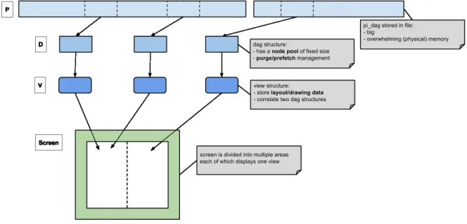
There can be multiple views based on the same DAG, as well as there can be multiple Vs referencing the sameD. DAGVizalso supports multipleDs for the samePtoo, eachDexplore

diﬀerent parts ofPindependently. This kind of relationship betweenP,DandVare illustrated in Figure 3.1.

Figure 3.1. P-D-V design

In the following paragraphs, I’m going to describe detailed structures of P,D,V.

Structure of P P’s definition is shown in Figure A.1. Beside number of nodes, number of edges, the start clock of the execution, number of workers, a PIDAG holds a contiguous array of PIDAG’s nodes (Figure 3.3) which reference to the same dr dag node info structures with

DAG Recorder’s nodes but have diﬀerent linking structure between themselves as they are

flattened-down version ofDAG Recorder’s DAG. PIDAG’s nodes also have 5 kinds, they are

create,wait,end,sectionandtask(same asDAG Recorder’s node kinds) (Figure 1.4). section

and task are collective nodes which contain subgraphs inside them. All (direct) child nodes of a collective node are arranged contiguously in a sub-array somewhere behind the node in the array. So a sectionor a taskwould additionally hold two oﬀset indexes (subgraphs begin oﬀset,

subgraphs end oﬀset) pointing to the beginning and the end of the sub-array where their child

nodes reside. Acreatenode would additionally hold one oﬀset index pointing to thetask node that it creates. Figure 3.2 illustrates how nodes of a DAG offib(3) program would be arranged in PIDAG. As we can see from the figure, child nodes of a task reside right behind it. Child nodes of a section are put after the sub-array that that section belongs to. task node created

by acreatenode is inserted after the sub-array that contains that drcreate node.

Structure of D D structure’s definition is shown in Figure A.2. First of all, aD structure holds a pointer to the P that it associates with. Then, the most important part of a D is its

(27)

Figure 3.2. Flattened DAG Recorder’s nodes in PIDAG offib(3) program

1 structdr pi dag node{

2 dr dag node infoinfo;

3 longedges begin;/* index of begining of edges from this node */

4 longedges end;/* index of end of edges from this node */

5 union{

6 /* for create node */

7 longchild oﬀset; /* offset to its created task */

8 /* for section or task node */

9 struct{

10 longsubgraphs begin oﬀset;/* offset to beginning of subgraphs */

11 longsubgraphs end oﬀset;/* offset to end of subgraphs */

12 };

13 };

14 };

Figure 3.3. PIDAG’s node

node pool. The pool is a fixed-size array of DAGViz’s nodes (Figure A.4). It consists of T, To,Tsz, Tn member variables of the D. Its size stored in Tsz is currently set at one hundred thoundsand. To (T occupied) is used to indicate if a node in the arrayT has been allocated for the DAG. So To has the same number of elements as T does. Number of currently allocated nodes ofT is stored inTn. The allocation and releasing mechanisms of node pool are provided through following interfaces:

• dv dag node pool init(): initialize node pool’s variables to default values, allocate memory

for T array and To array.

• dv dag node pool is empty(): to check if the node pool is empty (occupied fully) or not by

comparing Tn with Tsz.

• dv dag node pool avail(): return the current number of available nodes in the pool (Tsz

−Tn).

• dv dag node pool pop(): return one pointer to an available node in the pool, set the flag

of that node as occupied in To. If the pool is empty, call the function dv dag clear shrin

ked nodes() to ask for D to release children of shrinked nodes in the DAG which are not

currently visible.

• dv dag node pool push(): used to return a node to the pool by reseting its occupied flag

(28)

• dv dag node pool pop contiguous(): used to pop a contiguous sub-array of nodes in T. The purpose of this function is that if all child nodes of a section or atask in Pare assigned contiguousD’s nodes, it makes it easier forDto later locate all child nodes of a particular node and release them to the pool when necessary.

Using these interfaces, D can acquire nodes from and return nodes to the pool in order to build its DAG in memory. Reversely, D also provides an interface, dv dag clear shrinked no

des(), for the pool to initiatively ask D to return unnecessary nodes for it to supply for new

allocation requests when it has run out of available nodes. The mechanism indv dag clear shrin

ked nodes()will be discussed in Section 3.2 when DAG’s structure based on the linking between

D’s nodes are described. Beside the node pool, a D also stores other parameters specifying its relative position inside P such as its current depth (cur d), its current depth including nodes that are extensible to but hidden (not visible) on screen (cur d ex).

Structure of V A V is associated with one D. V’s full definition is shown in Figure A.3. Its first member variable is a pointer to a D. V holds viewing parameters for the D that it is associated with. These viewing parameters can be classified into 3 categories of appearance, drawing and interaction parameters. Appearance parameters are:

• lt: layout type of the DAG

• et: edge type specifying how to draw edges

• edge aﬃx: indicates if an aﬃx segment of edge should be drawn at the contact of an edge

and a node

• nc: node color mode, indicate what to be represented by colors (worker, cpu, node kind or source code location)

Drawing parameters are:

• vpw, vph: width and height of the main viewport that thisVis displayed on. The notion

of viewport will be discussed in Section 3.6.1.

• x, y: position of the coordinate origin of the view in viewport, is changed when user pan the DAG around screen.

• zoom ratio x, zoom ratio y: zoom ratios for cairo to magnify/shrink graphics horizontally

and vertically

• nd: number of nodes drawn on screen

• ndh: number of nodes drawn on screen plus number of collective nodes not drawn on screen but needed to traverse through when drawing DAG

Interaction parameters are:

• focused: indicate if the view is focused or not so that hot keys would be eﬀective to it

• cm: clicking mode, indicate what to do when user clicks a node

• drag on: indicate if a dragging operation is being conducted or not

• pressx, pressy: position where the user presses (clicking down)

• accdisx, accdisy: accumulated moving distance since the user pressed

• do zoom x, do zoom y: indicate to make cairo do zooming when the user scroll on the

view

• do scale radix, do scale radius: change the radix and/or radius then make DAGViz

re-layout and re-draw the DAG. This results in magnifying/shrinking the DAG by re-laying out rather than the automatic cairo’s zooming.

(29)

1 typedef struct dv dag node{

2 ...

3 /* linking structure */

4 structdv dag node ∗parent;

5 structdv dag node ∗pre;

6 dv llist t links[1];

7 structdv dag node ∗head; 8 dv llist t tails[1];

9 ...

10 } dv node coordinate t;

Figure 3.4. Node’s linking variables

Common linked list data structure DAGVizimplements a common linked list data

struc-ture (dv llist t). This list structure provides such operations as add operation to add a new item to the end of the list, pop operation to pop the first item out of the list, get operation to get (but not remove) any item on the list using its index. The list element can store any kind of pointer (void *) as its item. For example, this list data structure is being used to hold the list ofP’s nodes that have info tags to draw (P→itl), the list ofD’s nodes having info tag (D→itl), the list ofDAGViz’s nodes that are in the middle of collapse/expand animation.

Automatic view coordination The fact that multiple Vs can reference the sameDmakes

these Vs coordinated automatically because any change that the user makes to theD through anyVwould propagate to otherVs too. The change can be some changing to the properties that

D structure has. It is the same that multipleDs referencing the samePwould be coordinated on the properties that Pstructure holds too. Moreover, all Vs that reference diﬀerentDs but theirDs reference the sameP would be coordinated on the properties that Pstructure holds.

3.2 DAG Structure and Hierarchical Traversal Model

In this section, we will discuss about how DAG structure is constructed based on linking between

D’s nodes. DAGViz considers “child nodes” notion of asectionwider thanDAG Recorder.

Child node group of asectionconsists of not onlycreate,section,waitnodes asDAG Recorder

does but also task nodes which child create nodes in the group create. Child nodes of a task

still consist of onlysection andend.

One node will hold five pointers or lists of pointers referencing to some other nodes related to it: parent, pre, links, head and tails in which links and tails are lists of nodes (Figure 3.4. These five variables can be described as below:

• parent: its parent node

• pre: the node right before it in the same group of child nodes of its parent. pre of atask

and continuation node is thecreatenode that created thetask.

• links: is a list of nodes that it links to. A node links to its next node in the same group of child nodes. Acreatenode links to the taskthat it created and its continuation node.

• head: the head one (or the first one) of its child nodes.

• tails: the last one of its child nodes and also all task nodes that its child create nodes create.

Because the DAG is a hierarchical structure with many levels of layers stacked upon each other, we can classify these variables as such that parent points to the higher layer, pre and

links point to nodes next to it in the same layer, head and tails point to child nodes in lower

(30)

Figure 3.5. Hierarchical layout model

The “linked” relationship between nodes in DAGViz is a superset of the “contiguous”

relationship between code segments. It is true that two nodes of two contiguous code segments are linked together but the reverse is not always true. For example, a create node and a task

node are linked but they are not contiguous in the application code.

A DAG begins with a singletasknode representing the whole original application. Beginning from this roottaskwe can traverse all nodes of the DAG recursively. A simplified version of this traversal model is shown in Figure 3.6a. At each node, after processing itself, it calls recursively its head node and then calls each of its linked (successor) nodes.

However, in some cases that simple traversal pattern is not enough because nodes sometimes require to be processed before they are traversed, or sometimes some of their processing need to be computed only after their inner subgraphs have been processed or after all their linked successors have been processed. In those cases, a more complex traversal model generalized in Figure 3.6b is needed.

At first, only the originaltasknode is accessed in PIDAG (for it to be loaded into physical), assigned a node inD’s node pool and rendered on the screen. This node and other child nodes later would get accessed, loaded and rendered based on the user’s demand. So state transition of a node can be systemized like this:

none→set→inner loaded

When a node has just been allocated from the pool and initialized, it has statenone. When the function dv dag node set() is called upon it, DAGViz would access its corresponding P’s node in PIDAG, causing it to be loaded into physical memory if it is not yet, and evaluate if it has any child node. If it has child node(s), it is considered a “union” node that can be expanded further into subgraphs. Even a or node which has been collapsed byDAG Recorder is not of “union” kind. A “union” node can move to the next state of inner loaded which indicates that all its child nodes have been accessed and loaded into D. A node in inner loaded state is switched betweenshrinked and expanded states which specifies if its inner subgraph should be drawn on screen or “collapsed” (this is visual collapse conducted byDAGViz, not the physical

collapse done by DAG Recorder).

shrinked↔expanded

In summary, a D’s node would hold following flags to specify its possible state transitions above, in which two flags ofexpanding andshrinking are used for the collapse/expand animation mechanism (Section 3.5).

(31)

1 inttraverse(dv dag node t∗ node){ 2 /* Process individual */ 3 visit(node); 4 /* Traverse inward */ 5 if(node−>head){ 6 traverse(node−>head); 7 } 8 /* Traverse link-along */

9 for(next innode−>links){

10 traverse(next);

11 } 12 }

(a) simple

1 inttraverse(dv dag node t∗ node){

2 /* Traverse inward */ 3 if(node−>head){ 4 /* Process head */ 5 ... 6 /* Traverse */ 7 traverse(node−>head);

8 /* Process node with inward */

9 ...

10 }else{

11 /* Process node without inward */

12 ...

13 }

14 /* Traverse link-along */

15 switch(node−>links.size()){

16 case0:

17 /* Process node without link-along */

18 ...

19 break;

20 case1:

21 /* Process one next */

22 ...

23 /* Traverse */

24 traverse(next);

25 /* Process node with one link-along */

26 ...

27 break;

28 case2:

29 /* Process two nexts */

30 ...

31 /* Traverse */

32 traverse(right next);

33 traverse(left next);

34 /* Process node with two link-alongs */

35 ...

36 } 37 }

(b) complex

DAGViz: A DAG Visualization Tool for Analyzing Task Parallel Programs (DAGViz: DAG )

修士論文