Video-Based People Tracking

Video-Based People Tracking

Marcus A. Brubaker, Leonid Sigal and David J. Fleet

1 Introduction

Vision-based human pose tracking promises to be a key enabling technology for myriad applications, including the analysis of human activities for perceptive envi-ronments and novel man-machine interfaces. While progress toward that goal has been exciting, and limited applications have been demonstrated, the recovery of hu-man pose from video in unconstrained settings remains challenging. One of the key challenges stems from the complexity of the human kinematic structure itself. The sheer number and variety of joints in the human body (the nature of which is an active area of biomechanics research) entails the estimation of many parameters. The estimation problem is also challenging because muscles and other body tissues obscure the skeletal structure, making it impossible to directly observe the pose of the skeleton. Clothing further obscures the skeleton, and greatly increases the vari-ability of individual appearance, which further exacerbates the problem. Finally, the imaging process itself produces a number of ambiguities, either because of occlu-sion, limited image resolution, or the inability to easily discriminate the parts of a person from one another or from the background. Some of these issues are inherent, yielding ambiguities that can only be resolved with prior knowledge; others lead to computational burdens that require clever engineering solutions.

The estimation of 3D human pose is currently possible in constrained situations, for example with multiple cameras, with little occlusion or confounding background clutter, or with restricted types of movement. Nevertheless, despite a decade of ac-Marcus A. Brubaker

Department of Computer Science, University of Toronto, e-mail:[email protected]. edu

Leonid Sigal

Department of Computer Science, University of Toronto, e-mail:[email protected] David J. Fleet

Department of Computer Science, University of Toronto, e-mail:[email protected] H. Nakashima et al. (eds.),Handbook of Ambient Intelligence and Smart Environments, 57 DOI 10.1007/978-0-387-93808-0_3, © Springer Science+Business Media, LLC 2010

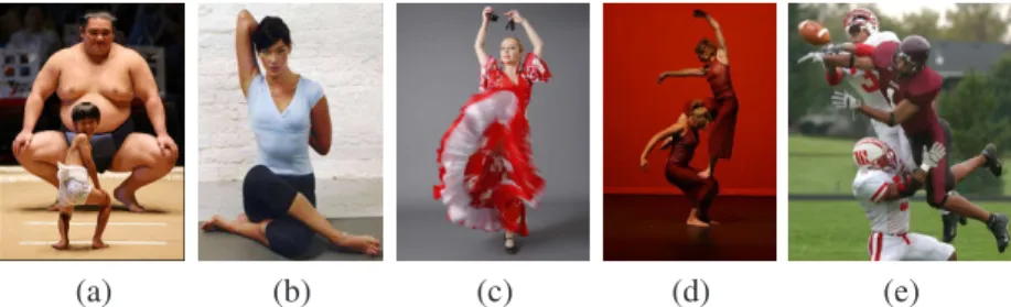
(a) (b) (c) (d) (e)

Fig. 1 Challenges in human pose estimation.Variation in body size and shape (a), occlusions of body parts (b), inability to observe the skeletal motion due to clothing (c), difficulty segmenting the person from the background (d), and complex interactions between people in the environment (e), are challenges that plague the recovery of human pose in unconstrained scenes.

tive research, monocular 3D pose tracking remains largely unsolved. From a single view it is hard to escape ambiguities in depth and scale, reflection ambiguities where different 3D poses produce similar images, and missing observations of certain parts of the body because of self-occlusions.

This chapter introduces the basic elements of modern approaches to pose track-ing. We focus primarily on monocular pose tracking with a probabilistic formula-tion. While multiview tracking in constrained settings, e.g., with minimal occlusion, may be relatively straightforward [29, 10] the problems faced in monocular tracking often arise in the general multiview case as well. This chapter is not intended to be a thorough review of human tracking but rather a tutorial introduction for practitioners interested in applying vision-based human tracking systems. For a more exhaustive review of the literature we refer readers to [17, 38].

1.1 Tracking as Inference

Because of the inescapable uncertainty that arises due to ambiguity, and the preva-lence of noisy or missing observations of body parts, it has become common to for-mulate human pose tracking in probabilistic terms. As such, the goal is to determine the posterior probability distribution over human poses or motions, conditioned on the image measurements (or observations).

Formally, letst denote the state of the body at timet. It represents the unknown

parameters of the model we wish to estimate. In our case it typically comprises the joint angles of the body along with the position and orientation of the body in world coordinates. We also have observations at each time, denotedzt. This might simply

be the image at timetor it might be a set of image measurements (e.g., edge loca-tions or optical flow). Tracking can then be formulated as the problem of inferring the probability distribution over state sequences,s1:t = (s1,...,st), conditioned on

the observation history,z1:t= (z1,...,zt); that is, p(s1:t|z1:t). Using Bayes’ rule, it

p(s1:t|z1:t) =

p(z1:t|s1:t)p(s1:t)

p(z1:t) .

(1) Here,p(z1:t|s1:t)is called the likelihood. It is the probability of observing the image

measurements given a state sequence. In effect the likelihood provides a measure of the consistency between a hypothetical motion and the given image measurements. The other major factor in (1) is the prior probability of the state sequence,p(s1:t).

This prior distribution captures whether a given motion is plausible or not. During pose tracking we aim to find motions that are both plausible and consistent with the image measurements. Finally, the denominator in (1), p(z1:t), often called the

partition function, does not depend on the state sequence, and is therefore considered to be constant for the purposes of this chapter.

To simplify the task of approximating the posterior distribution over human mo-tion (1), or of finding the most probable momo-tion (i.e., the MAP estimate), it is com-mon to assume that the likelihood and prior models can be factored further. For example, it is common to assume that the observations at each time are independent given the states. This allows the likelihood to be rewritten as a product of simpler likelihoods, one at each time:

p(z1:t|s1:t) = t

∏

i=1

p(zi|si). (2)

This assumption and resulting factorization allows for more efficient inference and easier specification of the likelihood. Common measurement models and likelihood functions are in Section 3.

The prior distribution over human motion also plays a key role. In particular, ambiguities and noisy measurements often necessitate a prior model to resolve un-certainty. The prior model typically involves a specification of which poses are plau-sible or implauplau-sible, and which sequences of poses are plauplau-sible. Often this involves learning dynamical models from training data. This is discussed in Section 4.

The last two elements in a probabilistic approach to pose tracking are inference and initialization. Inference refers to the process of finding good computational ap-proximations to the posterior distribution, or to motions that are most probable. This is discussed in Section 5. Furthermore, tracking most often requires a good initial guess for the pose at the first frame, to initialize the inference. Section 6 discusses methods for automatic initialization of tracking and for recovery from tracking fail-ures.

2 Generative Model for Human Pose

To begin to formulate pose tracking in more detail, we require a parameterization of human pose. While special parameterizations might be required for certain tasks, most approaches to pose tracking assume an articulated skeleton, comprising con-nected, rigid parts. We also need to specify the relation between this skeleton and

p

ο

r

i

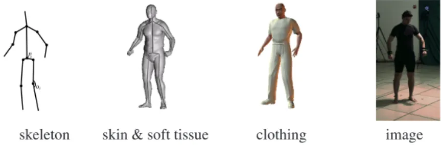
skeleton skin & soft tissue clothing image

Fig. 2 Simple image formation model for a human pose.The skeleton of the human body is overlaid with soft tissue and clothing. Furthermore, the formation of an image of the person (on the right) also depends on lighting and camera parameters.

the image observations. This is complex since we do not observe the skeleton di-rectly. Rather, as illustrated in Figure 2, the skeleton is overlaid with soft tissue, which in turn is often covered by clothes. The image of the resulting surface also then depends on the viewpoint of the camera, the perspective projection onto the image plane, the scene illumination and several other factors.

2.1 Kinematic Parameterization

An articulated skeleton, comprising rigid parts connected by joints, can be repre-sented as a tree. One part, such as the upper torso, is defined to be the root node and all remaining parts are either a child of the root or of another part. In this way, the entire pose can be described by the position and orientation of the root node in a global coordinate frame, and the position and orientation of each part in the coordi-nate frame of its parent. The statesthen comprises these positions and orientations. If parts are rigidly attached at joints then the number of degrees of freedom (DOFs) required will be less than the full 6 DOFs necessary to represent pose in a 3D space. The precise number of degrees of freedom varies based on the type of joint. For instance, a hinge joint is commonly used to represent the knee and has one rotational DOF while a ball-and-socket joint, often used to represent the hip, has three rotational DOFs. While real joints in the body are significantly more complex, such simple models greatly reduce the number of parameters to estimate.

One critical issue when designing the state space is the parameterization of ro-tations. Formally, rotations inR3are 3×3 matrices with determinant 1, the set of which is denotedSO(3). Unfortunately, 3×3 matrices have significantly more pa-rameters than necessary to specify the rotation, and it is extremely difficult to keep a matrix inSO(3)as it changes over time. Lower dimensional parameterizations of rotations are therefore preferred. Most common are Euler angles, which represent a rotation as a sequence of 3 elementary rotations about fixed axes. Unfortunately, Euler angles suffer from several problems including ambiguities, and singularities

known as Gimbal lock. The most commonly used alternatives include exponential maps [21] and quaternions [34].

2.2 Body Geometry

The skeleton is overlaid with soft tissue and clothing. Indeed we do not observe the skeleton but rather the surface properties of the resulting 3D volume. Both the geometry and the appearance of the body (and clothing) are therefore critical factors in the estimation of human pose and motion.

Body geometry has been modeled in many ways and remains a largely unex-plored issue in tracking and pose estimation. A commonly used model treats the segments of the body as rigid parts whose shapes can be approximated using sim-ple primitives such as cylinders or ellipsoids. These geometric primitives have the advantage of being simple to design and efficient to work with under perspective projection [64, 73]. Other, more complex shape models have been used such as de-formable super-quadrics [37], and implicit functions comprising mixtures of Gaus-sian densities to model 3D occupancy [47]. The greater expressiveness allows one to more accurately model the body, which can improve pose estimation, but it in-creases the number of parameters to estimate, and the projection of the body onto the image plane becomes more computationally expensive.

Recent efforts have been made to build detailed models of shape in terms of deformable triangulated meshes that are anchored to a skeleton. A well-known ex-ample of which is the SCAPE model [2]. By using dimensionality reduction, the triangulated mesh is parameterized using a small number of variables, avoiding the potential explosion in the number of parameters. Using multiple cameras one can accurately recover both the shape and pose [4]. However, the computational cost of such models is high, and may only be practical with offline processing. Good results on 3D monocular hand tracking have also been reported, based on a mesh-based sur-face model with approximately 1000 triangular sur-facets [11].

However, even deformable mesh body models cannot account for loose fitting clothing. Dresses and robes are extreme examples, but even loose fitting shirts and pants can be difficult to handle, since the relationship between the surface geometry observed in the image and the underlying skeleton is very complex. In most current tracking algorithms, clothing is assumed to be tight fitting so that the observed ge-ometry is similar to the underlying body. To handle the resulting errors due to these assumptions, the observation models (and the likelihood functions) must be robust to the kinds of appearance variations caused by clothing. Some have attempted to explicitly model the effects of clothing and its interaction with the body to account for this, but these models are complex and computationally costly [3, 54]. This re-mains a challenging research direction.

2.3 Image Formation

Given the pose and geometry of the body, the formation of an image of the per-son depends on several other factors. These include properties of the camera (e.g., the lens, aperture and shutter speed), the rest of the scene geometry (and perhaps other people), surface reflectance properties of clothing and background objects, the illumination of the scene, etc. In practice much of this information is unavail-able or tedious to acquire. The exception to this is the geometric calibration of the camera. Standard methods exist (e.g., Forsyth and Ponce [16]) which can estimate camera parameters based on images of calibration targets.1_{With fixed cameras this}

need only be done once. If the camera moves then certain camera parameters can be included in the state, and estimated during tracking. In either case, the camera parameters define a perspective projection,P(X), which maps a 3D pointX∈R3_to

a point on the 2D image plane.

3 Image Measurements

Given the skeleton, body geometry and image formation model, it remains to for-mulate the likelihood distributionp(z|s)in (1).2Conceptually, the observations are the image pixels, and the likelihood function is derived from ones generative model that maps the human pose to the observed image. As suggested in Figure 2, this involves modeling the surface shape and reflectance properties, the sources of illu-mination in the scene, and a photo-realistic rendering process for each pixel. While this can be done for some complex objects such as the human hand [11], this is extremely difficult for clothed people and natural scenes in general. Many of the necessary parameters about scene structure, clothing, reflectance and lighting are unknown, difficult to measure and not of direct interest. Instead, approximations are used that explain the available data while being (to varying degrees) independent of many of these unknown parameters. Toward that end it is common to extract a collection of image measurements, such as edge locations, which are then treated as the observations. This section briefly introduces the most common measurements and likelihood functions that are often used in practice.

3.1 2D Points

One of the simplest ways to constrain 3D pose is with a set image locations that are projections of known points on the body. These 3D points might be joint centers or 1_{Standard calibration code and tools are available as part of OpenCV (The Open Computer Vision}

Library), available fromhttp://sourceforge.net/projects/opencvlibrary/.

points on the surface of the body geometry. For instance, it is easy to show that one can recover 3D pose up to reflection ambiguities from the 2D image positions to which the joint centers project [66].

If one can identify such points (e.g., by manual initialization or ensuring that subjects wear textured clothing that produce distinct features), then the observation zcomprises a set of 2D image locations,{mi}Mi=1, where measurementmi

corre-sponds to locationion partj(i). If we assume that the 2D image observations are

corrupted by additive noise then the likelihood function can be written as p({mi}Mi=1|s) = M

∏

position in the global coordinate frame of the pointon part jgiven the current state s. The functionpi(d)is the probability density function of mean-zero additive noise

on pointi. This is often chosen to be Gaussian with a standard deviation ofσi, i.e.,

pi(d) = 1 √ 2π σi exp −d2 2σ_i2 . (4)

However, if it is believed that some of the points may be unreliable, for instance if they are not tracked reliably from the image sequence, then it is necessary to use a likelihood density withheavy tails, such as a Student’s t-distribution. The greater probability density in the tails reflects the belief that measurement outliers exist, and reduces the influence of such outliers in the likelihood function.

One way to find the image locations to which the joint centers project is to detect and track a 2D articulated model [15, 51, 58]; unfortunately this problem is almost as challenging as the 3D pose estimation problem itself. Another approach is to find image patches that are projections of points on the body (possibly joint centers), and can be reliably tracked over time, e.g., by the KLT tracker [67] or the WSL tracker [28]. Such a likelihood is easy to implement and has been used effectively [69, 70]. Nevertheless, acquiring 2D point tracks frequently requires hand initialization and tuning of the tracking algorithm. Further, patch trackers often fail when parts are occluded or move quickly, requiring reinitialization or other modifications to maintain a reliable set of tracks.

3.2 Background Subtraction

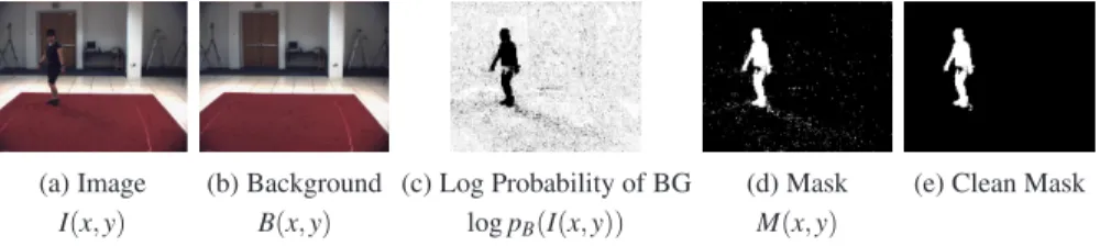
If the camera is in a fixed location and the scene is relatively static, then it is rea-sonable to assume that a background imageB(x,y)of the scene can be acquired (see Figure 3 (b)). This can then be subtracted from an observed imageI(x,y)and thresholded to determine a mask that indicates which pixels correspond to the fore-ground person [23, 49]. That is,M(x,y) =1 ifI(x,y)−B(x,y)>εandM(x,y) =0

(a) Image (b) Background (c) Log Probability of BG (d) Mask (e) Clean Mask I(x,y) B(x,y) logpB(I(x,y)) M(x,y)

Fig. 3 Background subtraction. Original image is illustrated in (a); the corresponding back-ground image of the scene, B(x,y), in (b); (c) shows the log probability of each pixelI(x,y) belonging to the background (with light color corresponding to high probability); (d) illustrates the foreground mask (silhouette image) obtained by thresholding the probabilities in (c); in (e) a cleaned up version of the foreground mask in (d) obtained by simple morphological operations.

otherwise (e.g. Figure 3 (d)). The mask can be used to formulate a likelihood by pe-nalizing discrepancies between the observed mask M(x,y) and a mask ˆM(x,y|s) predicted from the image projection of the body geometry. For instance Deutscher and Reid [13] used

p(M|s) =

∏

whereσcontrols how strongly disagreements are penalized. Such a likelihood is at-tractive for its simplicity but there will be significant difficulty in setting the thresh-oldεto an appropriate value; there may be no universally satisfactory value.

One can also consider a probabilistic version of background subtraction which avoids the need for a threshold (see Figure 3 (c)). Instead, it is assumed that back-ground pixels are corrupted with mean-zero, additive Gaussian noise. This yields the likelihood function

p(I|s) =

∏

pB(I(x,y))1−Mˆ(x,y|s) (6)

where pB(I(x,y))is the probability that pixelI(x,y) is consistent with the

back-ground. For instance, a hand specified Gaussian model can be used or more complex models such as mixtures of Gaussians can be learned in advance or during tracking [63]. Such a likelihood will be more effective than one based on thresholding.

Nevertheless, background models will have difficulty coping with body parts that appear similar to the background; in such regions, like the lower part of the torso in Figure 3, the model will be penalized incorrectly. Problems also arise when limbs occlude the torso or other parts of the body, since then one cannot resolve them from the silhouette. Finally, background models often fail when the illumination changes (unless an adaptive model is used), when cameras move, or when scenes contain moving objects in the background.

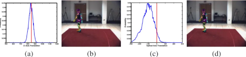
500 600 700 800 900 1000 1100 1200 0 0.005 0.01 0.015 0.02 0.025 0.03 0.035 0.04 0.045 Z−Axis Translation Probability −3000 −200 −100 0 100 200 300 0.002 0.004 0.006 0.008 0.01 0.012 0.014 0.016 0.018 0.02

Optical Axis Translation

Probability

(a) (b) (c) (d)

Fig. 4 Background likelihood.The behavior of the background subtraction likelihood described by Equation (5) is illustrated. A true pose, consistent with the pose of the subject illustrated in Figure 3, is taken and the probability of that pose as a function of varying a single degree of freedom in the state are illustrated in (a) and (c); in (a) the entire body is shifted up and down (along the Z-axis), in (d) along the optical axis of the camera. In (b) and (d) poses corresponding to the strongest peak in the likelihood of (a) and (c) respectively are illustrated. While ideally one would prefer the likelihood to have a single global maxima at the true value (designated by the vertical line in (a) and (c)), in practice, the likelihoods tend to be noisy, multi-modal and may not have a peak in the desired location. In particular in (c), due to the insensitivity of monocular likelihoods to depth, noise in the obtained foreground mask and inaccuracies in the geometric model of the body lead to severe problems. Also note that, in both figures, the noise in the likelihood indicates that simple search methods are likely to get stuck in local optima.

3.3 Appearance Models

In order to properly handle uncertainty, e.g., when some region of the foreground appears similar to the background, it is useful to explicitly model the foreground appearance. Accordingly, the likelihood becomes

p(I|s) =

∏

pB(I(x,y))1−Mˆ(x,y|s)pF(I(x,y)|s)Mˆ(x,y|s) (7)

wherepF(I(x,y)|s)is the probability of pixelI(x,y)belonging to the foreground.

Notice that if a uniform foreground model is assumed, i.e.,pF(·)∝1, then (7) simply

becomes the probabilistic background subtraction model of (6).

An accurate foreground modelpF(I(x,y)|s)is often much harder to develop than

a background model, because appearance varies depending on surface orientation with respect to the light sources and the camera, and due to complex non-rigid de-formation of the body and clothing over time. It therefore requires offline learning based on a reasonable training ensemble of images [27, 50] or it can be updated online [76]. Simple foreground models are often learned from the image pixels to which the body projects to in one or more frames. For example one could learn the mean RGB color and the its covariance for the body, or for each part of the body if they differ in appearance. One can also model the statistics of simple filter outputs (e.g., gradient filters).

One important consideration about likelihoods is computational expense, as eval-uating every pixel in the image can be burdensome. Fortunately, this can usually be avoided as a likelihood function typically needs only be specified up to a multi-plicative constant. By dividing the likelihood by the background model for each

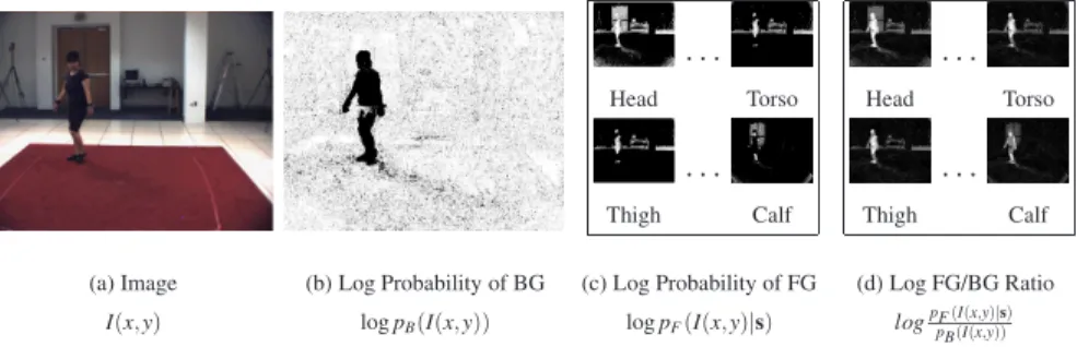
· · · Head Torso · · · Thigh Calf · · · Head Torso · · · Thigh Calf (a) Image I(x,y) (b) Log Probability of BG logpB(I(x,y)) (c) Log Probability of FG logpF(I(x,y)|s) (d) Log FG/BG Ratio logpF(I(x,y)|s) pB(I(x,y))

Fig. 5 Modeling appearance.The appearance likelihood described by Equation (8) is illustrated. The observed image is shown in (a); the log probability of a pixel belonging to the background in (b); the probability of the pixel belonging to a foreground model (modeled by a mixture of Gaus-sians) for a given body part in (c); the final log ratio of the foreground to background probability is illustrated in (d). Notice that unlike the background likelihood, the appearance likelihood is able to attribute parts of the image to individual segments of the body.

500 600 700 800 900 1000 1100 1200 0 0.005 0.01 0.015 0.02 0.025 0.03 0.035 0.04 Z−Axis Translation Probability −3000 −200 −100 0 100 200 300 0.002 0.004 0.006 0.008 0.01 0.012

Optical Axis Translation

Probability

(a) (b) (c) (d)

Fig. 6 Appearance likelihood.The behavior of the appearance likelihood described by Equation (8) is illustrated. Similarly to Figure 4 a true pose, consistent with the pose of the subject illustrated in Figure 3, is taken and the probability of that pose as a function of varying a single degree of free-dom in the state are illustrated in (a) and (c); as before in (a) the entire body is shifted up and down (along the Z-axis), in (d) along the optical axis of the camera. In (b) and (d) poses corresponding to the strongest peak in the likelihood of (a) and (c) respectively are illustrated. Notice that due to the strong separation between foreground and background in this image sequence, appearance likeli-hood performs similarly to the background likelilikeli-hood model (illustrated in Figure 4); in sequences where foreground and background contain similar colors appearance likelihoods tend to produce superior performance.

pixel terms cancel out leaving

p(I|s)∝

∏

pF(I(x,y)|s)

pB(I(x,y))

(8)

where the product is only over the foreground pixels, allowing a significant savings in computation. This technique can be more generally used to speed up other types of likelihood functions.

3.4 Edges and Gradient Based Features

Unfortunately foreground and background appearance models have several prob-lems. In general they have difficulty handling large changes in appearance such as those caused by varying illumination and clothing. Additionally, near boundaries they can become inaccurate since most foreground models do not capture the shad-ing variations that occur near edges, and the pixels near the boundary are a mixture of foreground and background colors due to limited camera resolution. For this rea-son, and to be relatively invariant to lighting and small errors in surface geometry, it has been common to use edge-based likelihoods [73]. These models assume that the projected edges of the person should correspond to some local structure in image intensity.

Perhaps the simplest approach to the use of edge information is the Chamfer dis-tance [5]. or the Hausdorff disdis-tance [25]. Edges are first extracted from the observed image using standard edge detection methods [16] and a distance map is computed whered(x)is the squared Euclidean distance from pixelxto the nearest edge pixel. The outline of the subject in the image is computed and the boundary is sampled at a set of points{bi}Mi=1. In the case of Chamfer matching the likelihood function is

p(d|s) =exp −1 M M

∑

Chamfer matching is fast, as the distance map need only be computed once and is evaluated only at edge points. Additionally, it is robust to changes in illumination and other appearance changes of the subject. However it can be difficult to obtain a clean set of edges as texture and clutter in the scene can produce spurious edges. Gavrila and Davis [19] successfully used a variant of Chamfer matching for pose tracking. To minimize the impact of spurious edges they performed an outlier rejec-tion step on the pointsbi.

Chamfer matching is also robust to inaccuracies in the geometry of the subject. If the edges of the subject can be predicted with a high degree of accuracy, then predictive models of edge structure can be used. Kollnig and Nagel [32] built hand specified models which predicted large gradient magnitudes near outer edges of the target. Later, this work was extended to predict gradient orientations and applied to human pose tracking by Wachter and Nagel [73]. Similarly, Nestares and Fleet [43] learned a probabilistic model of local edge structure which was used by Poon and Fleet [48] to track people. Such models can be effective however sufficiently accurate shape models can be difficult to build.

−3000 −200 −100 0 100 200 300 0.002 0.004 0.006 0.008 0.01 0.012 0.014 0.016 0.018 0.02

Optical Axis Translation

Probability −3000 −200 −100 0 100 200 300 0.01 0.02 0.03 0.04 0.05 0.06 0.07 0.08

Optical Axis Translation

Probability −3000 −200 −100 0 100 200 300 0.02 0.04 0.06 0.08 0.1 0.12 0.14

Optical Axis Translation

Probability

(1 view) (2 views) (3 views)

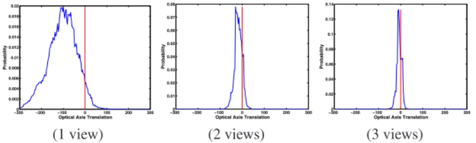
Fig. 7 Number of views.Effect of combining measurements from a number of image views on the (background) likelihood. With a single view the likelihood exhibits a wide noisy mode relatively far from the true value of the translation considered (denoted by the vertical line); with more views contributing image measurements the ambiguity can be resolved, producing a stronger peak closer to the desired value.

3.5 Discussion

There is no consensus as to which form of likelihood is best. However, some cues are clearly more powerful than others. For instance, if 2D points are practical in a given application then they should certainly be used as they are an extremely strong cue. Similarly, some form of background model is invaluable and should be used whenever it is available.

Another effective technique is to use multiple measurements. To correctly com-bine measurements, the joint probability of the two observations p(z(1),z(2)|s) needs to be specified. This is often done by assuming the conditional independence of the observations

p(z(1),z(2)|s) =p(z(1)|s)p(z(2)|s). (10) This assumption, often referred to asnaïve Bayes, is unlikely to hold as errors in one observation source are often correlated with errors in others. However, it is reason-able when, for instance, the two observations are from different cameras or when one set of observations is explaining edges and the other is explaining pixels not at the boundary. The behavior of the background likelihood (previously illustrated in Figure 4) as a function of image measurements combined from multiple views is illustrated in Figure 7.

4 Motion Models

Prior information about human pose and motion is essential for resolving ambi-guity, for combining noisy measurements, and for coping with missing observa-tions. A prior model biases pose estimation toward plausible poses, when pose might otherwise be under-constrained. In principle one would like to have priors that are weak enough to admit all (or most) allowable motions of the human body,

but strong enough to constrain ambiguities and alleviate challenges imposed by the high-dimensional inference. The balance between these two competing goals is of-ten elusive. This section discusses common forms of motion models and introduces some emerging research directions.

4.1 Joint Limits

The kinematic structure of the human body permits a limited range of motion in each joint. For example, knees cannot hyperextend and the torso cannot tilt or twist arbitrarily. A central role of prior models is to ensure that recovered poses satisfy such biomechanical limits. While joint limits can be encoded by thresholds imposed on each rotational DOF, the true nature of joint limits in the human body is more complex. In particular, the joint limits are dynamic and dependant on other joints [22]. Unfortunately, joint limits by themselves do not encode enough prior knowl-edge to facilitate tractable and robust inference.

4.2 Smoothness and Linear Dynamical Models

Perhaps the simplest commonly used prior model is a low-order Markov model, based on an assumption that human motion is smooth [73, 56, 48]. A typical first-order model specifies that the pose at one time is equal to the previous pose up to additive noise:

st+1 = st+η (11)

where theprocess noiseηis usually taken to be Gaussianη∼ N(0,Σ). The result-ing prior is then easily shown to be

p(st+1|st) = G(st+1;st,Σ) (12)

whereG(x;m,C)is the Gaussian density function with meanmand covarianceC, evaluated atx. Second-order models expressst+1in terms of ofstandst−1, allowing

one to use velocity in the motion model. For example, a common, damped second-order model is

st+1 = st+κ(st−st−1) +η (13)

whereκis a damping constant which is typically between zero and one.

Equations (11) and (13) are instances of linear models, the general form of which isst+1=∑Nn=1Anst−n+1+η, i.e., anN-th order linear dynamical model. In many

cases, as in (11) and (13), it is common to set the parameters of the transition model by hand, e.g., settingAn, assuming a fixed diagonal covariance matrixΣ, or letting

the diagonal elements of the covariance matrix in (12) be proportional to||st−st−1||2

would allow one, for example, to capture the coupling between different joints. Nev-ertheless, learning good parameters is challenging due to the high-dimensionality of the state space, for which the transition matrices,An∈RN×N, can easily suffer from

over-fitting.

Smoothness priors are relatively weak, and as such allow a diversity of motions. While useful, this is detrimental when the model is too weak to adequately constrain tracking in monocular videos. In constrained settings, where observations from 3 or more cameras are available and occlusions are few, such models have been shown to achieve satisfactory performance [13].

It is also clear that human motion is not always smooth, thereby violating smooth-ness assumptions. Motion at ground contact, for example, is usually discontinuous. One way to accommodate this is to assume a heavy-tailed model of process noise that allows occasional, large deviations from the smooth model. One might also consider the use of switching linear dynamical models, which produce piece-wise linear motions [46].

4.3 Activity Specific Models

Assuming that one knows or can infer the type of motion being tracked, or the identity of the person performing the motion, one can apply stronger prior models that are specific to the activity or subject [35]. The most common approach is to learn models off-line (prior to tracking) from motion capture data. Typically one is looking for some low-dimensional parameterization of the pose and motions.

To introduce the idea, consider a datasetΨ={ψ(i)_{}consisting ofK kinematic}

poses ψ(i)_{, i∈(1,...,K) obtained, for example, using a motion capture system.}

Since humans often exhibit characteristic patterns of motion, these poses will of-ten lie on or near a low-dimensional manifold in the original high-dimensional pose space. Using such data for training, methods like Principle Component Analysis (PCA) can be used to approximate poses by the linear combination of a mean pose

μΨ =K1∑ K

i=1ψ(i)and a set of learned principal directions of variation. These

prin-ciple directions are computed using the singular value decomposition (SVD) of a matrixSwhosei-th row isψ(i)−μ_Ψ. Using SVD, matrixSis decomposed into two orthonormal matricesU andV (U= [u1,u2,...,um]consisting of the eigenvectors,

(a.k.a.,eigen-poses) and a diagonal matrixΛ containing ordered eigenvalues such thatS=UΛVT.

Given this learned model, a pose can be approximated by

ψ≈μΨ+

q

∑

i=1

uici (14)

whereci is the set of scalar coefficients andqmcontrols the amount of

vari-ance accounted for by the model. As such, the inference over the pose can be re-placed by the inference over the coefficientss= [c1,c2,...,cq]. Sinceqis typically

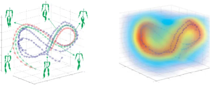
Fig. 8 Illustration of the latent space motion prior model.Results of learning a Gaussian Pro-cess Dynamical Model that encodes both the non-linear low-dimensional latent pose space and the dynamics in that space. On the left a few walking motions are shown embedded in the 3D latent space. Each point on a trajectory is an individual pose. For six of the points the corresponding mean pose in the full pose space is shown. On the right the distribution over plausible poses in the latent space is shown. This figure is re-printed from [74].

small (e.g. 2−5) with respect to the dimensionality of the pose space this transfor-mation facilitates faster pose estitransfor-mation. However, the new low-dimensional state space representation also requires a new model of dynamics that has to operate on the coefficients. The models of dynamics in the linear latent-space such as the one obtained using the eigen-decomposition are typically more complex then those in the original pose space and are often nonlinear. One alternative to simplifying the motion models is to learn the eigen-decomposition for entire trajectories of motion rather then the individual poses [56, 71]. Regardless, linear models such us the one described here are typically insufficient to capture intricacies of real human poses or motion.

More recent methods have shown that non-linear embeddings are more effective [60]. Gaussian Processes Latent Variable Models (GPLVMs) have became a popular choice since they have been shown to generalize from small amounts of training data [69]. Furthermore, one can learn a low-dimensional embedding that not only models the manifold for a given class of motions, but also captures the dynamics in that learned manifold [36, 70]. This allows the inference to proceed entirely in the low-dimensional space alleviating complexities imposed by the high-dimensional pose space all together. An example of a 3D latent space for walking motions is illustrated in Figure 8 and results of tracking with that model is shown in Figure 9.

Alternatively, methods that use motion capture directly to implicitly specify stronger priors have also been proposed. These types of priors make the assump-tion that the observed moassump-tion should be akin to the moassump-tion exhibited in the database of exemplar motions. Simply said, given a pose at timetsuch approaches find an ex-emplar motion from the database that contains a closely resembling pose, and uses that motion to look up the next pose in the sequence. Priors of this form can also be formulated probabilistically [57].

Fig. 9 Tracking with the GPDM.56 frames of a walking motion that ends with almost total occlusion (just the head is visible) in a cluttered and moving background. Note how the prior encourages realistic motion as occlusion becomes a problem. This figure is re-printed from [70].

All of these methods have proven effective for monocular pose inference in spe-cific scenarios for relatively simple motions. However, due to their action spespe-cific nature, learning models that successfully generalize and represent multiple motions and transitions between those motions has been limited.

4.4 Physics-based Motion Models

Recently, there has been preliminary success in using physics-based motion mod-els as priors. Physics-based modmod-els have the potential to be as generic as simple smoothness priors but more informative. Further, they may be able to recover sub-tleties of more realistic motion which would be difficult, if not impossible, with existing motion models. The use of physics-based prior models in human tracking dates back to the early 1990’s with pioneering work by Metaxas and Terzopoulos [37] and Wren and Pentland [75]. However, it is only recently that success with monocular imagery has been shown.

The fundamental motivation for physics-based motion models is the possibility that motions are best described by the forces which generated them, rather than a sequence of kinematic poses. These forces include not only the internal (e.g., mus-cle generated) forces used to propel limbs, but also external forces such as gravity, ground reaction forces, friction and so on. Many of these forces can be derived from first principles and provide important constraints on motion. Modeling the remain-ing forces, either deterministically or stochastically is then the central difficulty of physics-based motion models. This class of models remains a promising but rela-tively unexplored area for future research.

The primary difficulty with physics-based models is the instability of complex dynamical systems. Sensitivity to initial conditions, discontinuities of motion and other non-linearities have made robust, realistic control of humanoid robots an elu-sive goal of robotics research. To address this in the context of tracking Brubaker, Fleet, and Hertzmann [8] used a simplified, physical model that is stable and easy to control. While this model was restricted to simple walking motions, the work was extended by Brubaker and Fleet [7] to a more complex physical model, capable

of a wider range of motions. An alternative strategy employed by Vondrak, Sigal, and Jenkins [72] used a motion capture database to guide the dynamics. Using in-verse dynamics, they solved for the forces necessary to mimic motions found in the database.

5 Inference

In a probablistic framework our goal is to compute some approximation to the dis-tribution p(s1:t|z1:t). Often this is formulated as online inference, where the

distri-bution is computed one frame at a time as the observations arrive, exploiting the well-known recursive form of the posterior (assuming conditional independence of the observations):

p(s1:t|z1:t) ∝ p(zt|st)p(st|s1:t−1)p(s1:t−1|z1:t−1). (15)

The motion model,p(st|s1:t−1), is often a first order Markov model which simplifies

top(st|st−1). While this is not strictly necessary for the inference methods presented

here, it is important because the motion model then depends only on the last state as opposed to the entire trajectory.

The classic, and perhaps simplest, approach to this problem is the Kalman filter [73]. However, the Kalman Filter is not suitable for human pose tracking where the dynamics are non-linear and the likelihood functions are non-Gaussian. As a consequence, Sequential Monte Carlo techniques are amongst the most commonly used to perform this inference. Sequential Monte Carlo methods were first applied to visual tracking with the CONDENSATION algorithm of Isard and Blake [26] but were applied earlier for time series analysis by Gordon, Salmond, and Smith [20] and Kong, Liu, and Wong [33]. For a more detailed discussion of Sequential Monte Carlo methods, we refer the reader to the review article by Doucet, Godsill, and Andrieu [14].

In this section, we present a very simple algorithm, particle filtering, in which stochastic simulation of the motion model is combined with weighting by the likeli-hood to produce weighted samples which approximate the posterior. We also present two variants which attempt to work around the deficiencies of the basic particle fil-ter.

5.1 Particle Filter

A particle filter represents a distribution with a weighted set of sample states, de-noted{(s(_1:i)_t,w_1:(i)_t)|i=1,...,N}. When the samples arefairly weighted, then sample statistics approximate expectation under the target distribution, i.e.,

N

∑

w(_1:i)_t is the normalized weight. The sample statistics approach that of the target distribution as the number of samples,N, increases.

In a simple particle filter, given a fairly weighted sample set from timet, the samples at time t+1 are obtained withimportance sampling. First samples are drawn from a proposal distributionq(s_t(₊i)₁|s_1:(i)_t,z1:t+1). Then the weights are updated

w_1:(i)_t+1 = w_1:(i)_tp(zt+1|s (i) t+1)p(s (i) t+1|s (i) 1:t) q(s(_t+i)₁|s_1:(i)_t,z1:t+1) (17)

to be fairly weighted samples at timet+1. The proposal distribution must be non-zero everywhere the posterior is non-non-zero, but it is otherwise largely unconstrained. The simplest and most common proposal distribution is motion model,p(st+1|s1:t),

which simplifies the weight update to bew(_1:i)_t+1=w_1:(i)_tp(zt+1|s(_t+i)₁).

This simple procedure, while theoretically correct, is known to be degenerate. Astincreases, the normalized weight of one particle approaches 1 while the others approach 0. Weights near zero require a significant amount of computation but con-tribute very little to the posterior approximation, effectively reducing the posterior approximation to a point estimate.

To mitigate this problem, a resampling step is introduced where particles with small weights are discarded. Before the propagation stage a new set of samples

{˜s_1:(i)_t|i=1,...,N}is created by drawing an index jsuch thatp(j) =wˆ(_1:j_t), and then setting ˜s(_1:i)_t=s_1:(j_t). The weights for this new set of particles are then ˜w_1:(i)_t=1/Nfor alli. This resampling procedure can be done at every frame, at a fixed frequency, or only when heuristically necessary. While it may seem good to do this at every frame, as done by Isard and Blake [26], it can cause problems. Specifically, resampling introduces bias in finite sample sets, as the samples are no longer independent and can even exacerbate particle depletion over time.

Resampling when necessary balances the need to avoid degeneracy without in-troducing undue bias. One of the most commonly used heuristics is an estimate of theeffective sample size

Ne f f = N

∑

per-formed whenNe f f<Nthresh, otherwise it is skipped. The particle filtering algorithm,

Initialize the particle set{(s(₁i),w₁(i))|i=1,...,N} for t=1,2,... do

Compute the normalized weights ˆw(_1:i)_tand the effective number of samples

Ne f f as in (18)

if Ne f f <Nthreshthen

for i=1,...,N do

Randomly choose an index j∈(1,...,N)with probabilityp(j) =wˆ(_1:j_t) Set ˜s(_1:i)_t=s(_1:j_t)and ˜w(_1:i)_t=1

end for

Replace the old particle set{(s_1:(i)_t,w_1:(i)_t)|i=1,...,N}with

{(˜s(_1:i)_t,w˜_1:(i)_t)|i=1,...,N} end if

for i=1,...,N do

Samples(_ti₊)₁from the proposal distributionq(st+1|s(1:i)t,z1:t+1)

Construct the new state trajectorys(_1:i)_t+1= (s_1:(i)_t,s(_t+i)₁) Update the weightsw(_1:i)_t+1according to equation (17) end for

end for

Algorithm 1: Particle Filtering.

5.2 Annealed Particle Filter

Unfortunately, resampling does not solve all the problems of the basic particle filter described above. Specifically, entire modes of the posterior can still be missed, particularly if they are far from the modes of the proposal distribution or if modes are extremely peaked. One solution to this problem is to increase the number of particles, N. While this will solve the problem in theory, the number of samples theoretically needed is generally computationaly untenable. Further, many samples will end up representing uninteresting parts of the space. While these issues remain challenges, several techniques have been proposed in an attempt to improve the efficiency of particles filters. One approach, inspired by simulated annealling and continuation methods, is Annealed Particle Filtering (APF) [13].

The APF algorithm is outlined in Algorithm 2. At each timet, the APF goes through L levels of annealing. For each particle i, annealing level , begins by choosing a sample from the previous annealing level, s(_1:j_t)_+1,−1, with probability p(j) =wˆ(_1:i)_t+1,−1. The state at timet+1 of sample jis then diffused to create a new hypothesiss(_t+i)_1,according to

T(st+1,|s1:t+1,−1) =N(st+1,|st+1,−1,αΣ), (19)

Initialize the weighted particle set{(s(₁i_,)_L,w₁(i_,)_L)|i=1,...,N}. for t=1,2,... do

for i=1,...,N do

Samples(_ti₊)₁from the proposal distributionq(st+1|s(_1:i)_t,L,z1:t+1)

Construct the new state trajectorys(_1:i)_t+1,0= (s_1:(i)_t,L,s(_t+i)₁) Assign the weightsw(_1:i)_t+1,0= W0(s

(i) 1:t+1,0|z1:t+1) q(s(_t+i)_1,0|s_1:(i)_t,L,z1:t+1) end for for=1,...,L do for i=1,...,N do

Compute the normalized weights ˆ w(_1:i)_t+1,−1= ∑N j=1w( j) 1:t+1,−1 −1 w(_1:i)_t+1,−1

Randomly choose an index j∈(1,...,N)with probability p(j) =w(_1:j_t)_+1,−1

Samples(_ti₊)_1,from the diffusion distributionT(st+1,|s(1:jt)+1,−1)

Construct the new state trajectorys(_1:i)_t+1,= (s_1:(i)_t,s_t(₊i)_1,) Compute the annealed weightsw(_1:i)_t+1,=W(s_1:(i)_t+1,|z1:t+1)

end for end for end for

Algorithm 2: Annealed Particle Filtering.

W(s1:t+1,|z1:t+1) =

p(zt+1|st+1,)p(st+1,|st,)

_β

. (20)

In the aboveα ∈(0,1)is called the annealing rate and is used to control the scale of covariance,Σ, in the diffusion process. The β is the temperature parameter, derived based on the annealing rate,α, and the survival diagnostics of the particle set (for details see Deutscher and Reid [13]) to ensure that a fixed fraction of samples survive from one stage of annealing to the next.

The sequenceβ0,...,βL is a gradually increasing sequence between zero and

1, ending withβL=1. Whenβis small, the difference in height between peaks

and troughs of the posterior are attenuated. As a result it is less likely that one mode, by chance, will dominate and attract all the particles, thereby neglecting other, potentially important modes. In this way the APF allows particles to broadly explore the posterior in the early stages. This means that the particles are better able to find different potential peaks, which then attract the particles more strongly as the likelihood becomes more strongly peaked (asβincreases). It is worth noting that, withL=1, the APF reduces to the standard particle filter discussed in the previous section.

While often effective in finding significant modes of the posterior, the APF does not produce fairly weighted samples from the posterior. As such it does not

Fig. 10 Annealed Particle Filter (APF) tracking from multi-view observations.This figure is re-printed from [13].

Initialize{(s(₁i),w₁(i))|i=1,...,N} for t=1,2,... do

for i=1,...,N do

Sample ˜s(_ti₊)₁from the proposal distributionq(˜st+1|s(1:i)t,z1:t+1)

Construct the new state trajectory ˜s(_1:i)_t+1= (s1:t,s˜(t+i)1)

Update the weightsw(_1:i)_t+1according to equation (17) withs_t(₊i)₁=s˜(_ti₊)₁ end for

Compute the normalized weights ˆw(_1:i)_t+1=

∑N j=1w (j) 1:t+1 −1 w(_1:i)_t+1 for i=1,...,N do

Randomly choose an index j∈(1,...,N)with probabilityp(j) =wˆ(_1:j_t)₊₁. Set the target distribution to beP(q)∝p(zt+1|q)p(q|˜s(

j) 1:t)

Set the initial state of the Markov Chain toq0=˜st(+j)1

for r=1,...,R do

Sampleqrfrom the MCMC transition densityT(qr|qr−1), e.g., using

Hybrid Monte Carlo as described in Algorithm 4 end for

Sets(_1:i)_t+1= (˜s(_1:i)_t,qR)andw(_1:i)_t+1=1

end for end for

Algorithm 3: Markov Chain Monte Carlo Filtering.

accurately represent the posterior and the sample statistics of (16) are not repre-sentative of expectations under the posterior. Recent research has shown that by restricting the form of the diffusion and properly weighting the samples, one can obtain fairly weighted samples [18, 42].

5.3 Markov Chain Monte Carlo Filtering

Another way to improve the efficiency of particle filters is with the help of Markov Chain Monte Carlo (MCMC) methods to explore the posterior. A Markov Chain3 is a sequence of random variables q0,q1,q2,... with the property that for all i,

p(qi|q0,...,qi−1) =p(qi|qi−1). In MCMC, the goal is to construct a Markov Chain

chain such that, asiincreases,p(qi)approaches the desired target distributionP(q).

In the context of particle filtering at timet, the random variables,q, are hypothetical states st and the target distribution,P(q), is the posterior p(s1:t|z1:t). The key to

MCMC is the definition of a suitable transition densityp(qi|qi−1) =T(qi|qi−1). To

this end there are several properties that must be satisfied, one of which is

P(q) =

T(q|qˆ)P(qˆ)dqˆ . (21) This means that the chain has the target distributionP(q)as its stationary distribu-tion. For a good review of the various types of Markov transition densities used, and a more thorough introduction to MCMC in general, see [41].

A general MCMC-filtering algorithm is given in Algorithm 3. It begins by pro-pogating samples through time and updating their weights according to a conven-tional particle filter. These particles are then are chosen with probability proporconven-tional to their weights, as the initial states inNindependant Markov chains. The target dis-tribution for each chain is the posteriorp(st|,z1:t). The final states of each chain are

then taken to be fair samples from the posterior.

Choo and Fleet [9] used an MCMC method known as Hybrid Monte Carlo. The Hybrid Monte Carlo algorithm (Algorithm 4) is an MCMC technique, based on ideas developed for molecular dynamics, which uses the gradient of the posterior to efficiently find high probability states. A single step begins by sampling a vec-torp0∈Rmfrom a Gaussian distribution with mean zero and unit variance. Here

mis the dimension of the state vectorq0. The randomly drawn vector, known as

the momentem, is then used to perform a simulation of the system of differen-tial equations ∂_∂τp =−∂E_∂(_qq) and ∂_∂τq =pwhereτ is an artificial time variable and E(q) =−logP(q). The simulation begins at(q0,p0)and proceeds using a leapfrog

step which is explicitly given in Algorithm 4. There,L is the number of steps to simulate for andΔ is a diagonal matrix whos entries specify the size of step to take in each dimension of the state vectorq. At the end of the simulation, the ending state of the physical simulationqLis accepted with probabilitya=min(1,e−c)where

c= (E(qL) + 1 2p0 2_)−(E(q 0) + 1 2pL 2_{). (22)}

The specific form of the simulation procedure and the acceptance test at the end are designed such thatP(q)is the stationary distribution of the transition distribu-3_{A full review of MCMC methods is well beyond the scope of this chapter and only a brief}

Given a starting stateq0∈Rmand a target distributionP(q), define

E(q) =−logP(q).

Draw a momentum vectorp0∈Rmfrom a Gaussian distribution with mean 0

and unit variance. for=1,...,L do p−0.5=p−1−1₂Δ∂E(_∂q_q−1) q=q−1+Δp−0.5 p=p₋0.5−12Δ ∂E(q) ∂q end for

Compute the acceptance probabilitya=min(1,e−c)wherecis computed according to (22)

Setuto be a uniformly sampled random number between zero and one if u<a then

return qL

else

return q0

end if

Algorithm 4: Hybrid Monte Carlo Sampling.

tion. The parameters of the algorithm,Land the diagonals ofΔare set by hand. As a rule of thumbΔandLshould be set so that roughly 75% of transitions are accepted. An important caveat is that the values ofLandΔcannot be set based onqand must remain constant throughout a simulation. For more information on Hybrid Monte Carlo see [41].

6 Initialization and Failure Recovery

The final issue we must address concerns initialization and the recovery from track-ing failures. Because of the large number of unknown state variables one cannot assume that the filter can effectively search the entire state space without a good prior model (or initial guess). Fortunately, over the last few years, progress on the development of discriminative methods for detecting people and pose inference has been encouraging.

6.1 Introduction to Discriminative Methods for Pose Estimation

Fig. 11 Illustration of the simple discriminative model.The model introduced by [1] is illus-trated. From left to right the figure shows (1) silhouette image, (2) contour of the silhouette image, (3) shape context feature descriptor for a point on a contour, (4) a set of shape context descriptors in the high (60-dimensional) space, (5) a 100-dimensional vector quantized histogram of shape descriptors that is used to obtain (6) the pose of the person through linear regression. This figure is re-printed from [1].

training exemplars,D={(s(i),z(i))∼p(s,z)|i=1...N}), which are assumed to be fair samples from the joint distribution over states and measurements. The goal is to learn to predict an output for a given input. The inputs,z∈RM, are generic image measurements,4and outputss∈RN, as above, represent the 3D poses of the body. The simplest discriminative method is Nearest-Neighbor (NN) lookup [24, 39], where, given a set of features observed in an image, the exemplar from the training database with the closest features is found, i.e., k∗=arg minkd(z˜,z(k)). The pose

s(k∗)for that exemplar is returned. The main challenge is to define a useful similarity measured(·,·), and a fast indexing scheme. One such approach was proposed by Shakhnarovich, Viola, and Darrell [55]. Unfortunately, this simple approach has three drawbacks: (1) large training sets are required, (2) all the training data must be stored and used for inference, and (3) it produces unimodal predications and hence ambiguities (or multi-modality) in image-to-pose mappings cannot be accounted for (e.g., see Sminchisescu, Kanaujia, Li, and Metaxas [61]).

To address (1) and (2) a variety of global [1] and local [53] parametric models have been proposed. These models learn a functional mapping from image features to 3D pose. While these methods have been demonstrated successfully on restricted domains, and with moderately large training sets, they do not provide one-to-many mappings, and therefore do not cope with multi-modality.

Multi-modal mappings have been formulated in a probabilistic setting, where one explicitly models multi-modal conditional distributions,p(s|z,Θ), whereΘare pa-rameters of the mapping, learned by maximizing the likelihood of the training data

D. One example is the conditional Mixture of Experts (cMoE) model introduced by Sminchisescu, Kanaujia, Li, and Metaxas [61], which takes the form

p(s|z,Θ) =

K

∑

k=0

gk(z|Θ)ek(s|z,Θ), (23)

4_{For instance, histograms-of-oriented-gradients, vector quantized shape contexts, HMAX, spatial}

Fig. 12 Discriminative Output.Pose estimation results obtained using the discriminative method introduced by Kanaujia, Sminchisescu, and Metaxas. This figure is re-printed from [30].

whereKis the number of experts,gkare positive gating functions which depend on

the input features, andekare experts that predict the pose (e.g., kernel regressors).

This model under various incarnations has been shown to work effectively with large datasets [6] and with partially labeled data5[30].

The MoE model, however, still requires moderate to large amounts of training data to learn parameters of the gates and experts. Recently, methods that utilize an intermediate low dimensional embedding have been shown to be particularly effec-tive in dealing with little training data in this setting [40, 31]. Alternaeffec-tively, non-parametric approaches for handling large amounts of training data efficiently that can deal with multi-modal probabilistic predictions have also been recently pro-posed by Urtasun and Darrell [68]. Similar in spirit to the simple NN method above, their model uses the local neighborhood of the query to approximate a mixture of Gaussian Process (GP) regressors.

6.2 Discriminative Methods as Proposals for Inference

While discriminative methods are promising alternatives to generative inference, it is not clear that they will be capable of solving the pose estimation problem in a general sense. The inability to generalize to novel motions, deal with significant occlusions and a variety of other realistic phenomena seem to suggest that some generative component is required.

Fortunately, discriminative models can be incorporated within the generative set-ting in an elegant way. For example, multimodal conditional distributions that are the basis of most recent discriminative methods [6, 40, 61, 68] can serve directly as proposal distributions (i.e.,q(st+1|s1:t,z1:t+1)) to improve the sampling efficiency of

the Sequential Monte Carlo methods discussed above. Some preliminary work on 5_{Since joint samples span a very high dimensional space,R}N+M_{, obtaining a dense sampling of the}

joint space for the purposes of training is impractical. Hence, incorporating samples from marginal distributionsp(s)andp(z)is of great practical benefit.