A tree augmented classifier based on Extreme Imprecise Dirichlet Model

A tree augmented classifier based on Extreme Imprecise Dirichlet Model

G. Corani

⇑

, C.P. de Campos

IDSIA, Galleria 2, 6928 Manno-Lugano, Switzerland

a r t i c l e

i n f o

Article history:

Available online 22 August 2010 Keywords:

Imprecise Dirichlet Model Classification

TANC Naive credal Classifier

a b s t r a c t

We present TANC, a TAN classifier (tree-augmented naive) based on imprecise probabili-ties. TANC models prior near-ignorance via the Extreme Imprecise Dirichlet Model (EDM). A first contribution of this paper is the experimental comparison between EDM and the global Imprecise Dirichlet Model using the naive credal classifier (NCC), with the aim of showing that EDM is a sensible approximation of the global IDM. TANC is able to deal with missing data in a conservative manner by considering all possible completions (without assuming them to be missing-at-random), but avoiding an exponential increase of the computational time. By experiments on real data sets, we show that TANC is more reliable than the Bayesian TAN and that it provides better performance compared to pre-vious TANs based on imprecise probabilities. Yet, TANC is sometimes outperformed by NCC because the learned TAN structures are too complex; this calls for novel algorithms for learning the TAN structures, better suited for an imprecise probability classifier.

2010 Elsevier Inc. All rights reserved.

1. Introduction

Classification is the problem of predicting theclassof a given object, on the basis of some attributes (features) of it. A clas-sical example is the iris problem by Fisher: the goal is to correctly predict theclass, i.e., the species of Iris on the basis of four features (the length and the width of sepal and petal). In the Bayesian framework, classification is accomplished by updating a prior density (representing the beliefs before analyzing the data) with the likelihood (modeling the evidence coming from the data), in order to compute a posterior density over the classes, which is then used to select the most probable class.

The naive Bayes classifier (NBC)[1]is based on the ‘‘naive” assumption of stochastic independence of the features given the class; since the real data generation mechanism generally doesnotsatisfy such condition, this introduces a severe bias in the probabilities estimated by NBC. Yet, at least under the 0–1 loss, NBC performs surprisingly well[1,2]. Reasons for this phenomenon have been provided, among others, by Friedman[3], who proposed an approach to decompose the misclassi-fication error into bias error and variance error; the bias error represents how closely the classifier approximates the target function, while the variance error reflects the sensitivity of the parameters of the classifier to the training sample. Low bias and low variance are two conflicting objectives; for instance, NBC has high bias (because of the unrealistic independence assumption) but low variance, since it requires to estimate only a few parameters. The point was clearly made also by Domingos and Pazzani[1]who commented about NBC and C4.5 (a classifier with lower bias but higher variance than NBC’s): ‘‘A classifier with high bias and low variance will tend to produce lower zero-one loss than one with low bias and high variance, because only the variance’s effect will be felt. In this way, the naive Bayesian classifier can often be a more accurate classifier than C4.5, even if in the infinite-sample limit the latter would provide a better approximation. This effect should be especially visible at smaller sample sizes, since variance decreases with sample size. Indeed, Kohavi[4]has observed that the Bayesian classifier tends to outperform C4.5 on smaller data sets, and conversely for larger ones”.

0888-613X/$ - see front matter2010 Elsevier Inc. All rights reserved. doi:10.1016/j.ijar.2010.08.007

⇑Corresponding author.

E-mail addresses:[email protected](G. Corani),[email protected](C.P. de Campos).

Contents lists available atScienceDirect

International Journal of Approximate Reasoning

j o u r n a l h o m e p a g e : w w w . e l s e v i e r . c o m / l o c a t e / i j a r

Therefore, NBC can be accurate on small and medium data sets, but is then generally outperformed by more complex (i.e., less biased) classifiers on large data sets. A way to reduce the NBC bias is to relax the independence assumption using a more complex graph, like TAN (tree-augmented naive Bayes)[5]. In particular, TAN can be seen as a Bayesian network where each feature has the class as parent, and possibly also a feature as second parent. In fact, TAN is a compromise between general Bayesian networks, whose structure is learned without constraints and NBC, whose structure is determined in advance to be naive (i.e., each feature has the class as the only parent). TAN has been shown to outperform both general Bayesian networks and naive Bayes[5,6]. However the advantage of TAN over NBC is especially important on medium and large data sets, as predicted by the bias–variance analysis.

In this paper we develop acredalversion of TAN; the main characteristic of credal classifiers is that they return more classes when faced with aprior-dependent instance, i.e., when the most probable class of the instance varies with the prior adopted to induce the classifier. Credal classifiers face prior-dependent instances by returning a set of classes instead of a fragile single class, thus preserving reliability. They are based on a set of priors rather than on a single prior, which removes the arbitrariness involved in the choice of any single prior. The set of priors is modeled using the Impre-cise Dirichlet Model (IDM)[7]. The IDM satisfies a number of properties which are desirable to model prior ignorance

[8].1

Two IDM variants have been adopted in credal classifiers: theglobaland thelocalone. The global IDM allows to compute narrower intervals for upper and lower probabilities, but poses challenging computational problems. In fact, tractable algo-rithms for exactly computing upper and lower probabilities with the global IDM exist for the naive credal classifier[9], but not for general credal networks. On the other hand, the local IDM returns probability intervals which can be unnecessarily wide, but can be easily computed for any network structure.

Recently, the EDM (Extreme Dirichlet Model)[10]has been introduced, which restricts the global IDM to the extreme distributions. The intervals returned by the EDM are included (inner approximation) in the intervals returned by the global IDM. Interestingly, the EDM enables an easier computation of upper and lower probabilities, compared to the global IDM. Yet, the EDM has not been tested in classification; a first contribution of this paper is a thorough test of the EDM, carried out using the NCC: in particular, we have compared the ‘‘original” NCC of[9], based on the global IDM against NCC based on the EDM (NCC-EDM). The results show that NCC and NCC-EDM identically classify the large majority of instances, thus supporting the introduction of the EDM in credal classifiers as sensible and computationally tractable approximation of the global IDM.

However, besides prior ignorance, there is another kind of ignorance involved in the process of learning from data: igno-rance about the missingness process. Usually, classifiers ignore missing data; this entails the idea that the missingness pro-cess (MP) is non-selective in producing missing data, i.e., it is MAR (missing-at-random[11]). However, assuming MAR cannot be regarded as an objective approach if one is ignorant about the MP. By the term nonMAR we indicate not only that we cannot assume MAR, but more generally that we have no information about the MP. According to the Conservative Updating

Rule[12,13], in order to deal conservatively with nonMAR missing data, it is necessary to consider all the possible

replace-ments for missing data. The latest version of the naive credal classifier[14]does so.

In this paper we present TANC, a credal TAN which (a) models prior ignorance via the EDM and (b) treats missing data as nonMAR, by therefore considering all possible replacements. However, while the number of possible completions increase exponentially with the total number of missing data, the computational complexity of TANC remains affordable thanks to optimized algorithms. For the moment, TANC efficiently deals with nonMAR missing data in the training set; missing data in the test instance need to be completed in all possible ways, and thus the time increases exponentially in the number of such missing data. We leave for future work the development of an algorithm to deal efficiently with missing data in the test instance.

A credal TAN was already proposed in[15]; we refer to that algorithm as TANC*_{. TANC}*_{was based on the local IDM}

(prob-ably because of the difficulties to compute the global IDM) and returned a consider(prob-ably large number of indeterminate clas-sifications[15]. Moreover, TANC*_{did not deal with nonMAR missing data.}

We thoroughly evaluate TANC by experiments on 45 data sets; we compare TANC against the Bayesian TAN, showing that the accuracy of TAN sharply drops on the instances which are indeterminately classified by TANC. Then, we compare TANC with TANC*_{, via some metrics introduced in[16]to compare credal classifiers. In fact, TANC outperforms TANC}*_{; in}

particular, it is less indeterminate than TANC*_{, discovering some instances which can be safely classified with a single class}

and which were classified indeterminately by TANC*_{. Then, we compare TANC with NCC. It turns out that TANC is}

outper-formed by NCC on several data sets; the reason is that the TAN structure (learned using a traditional MDL algorithm) is sometimes too complex, causing TANC to become excessively indeterminate. We think that a novel algorithm for discover-ing the TAN structure may significantly improve the TANC performance by designdiscover-ing parameter-parsimonious structures; it could for instance use imprecise probabilities to cautiously decide whether to assign the second parent to a feature or not. However, there are also a few data sets where TANC does outperform NCC; they contain correlated variables and many in-stances, as predicted by the bias–variance analysis. Eventually, we present some preliminary results with nonMAR missing data; the performance of TANC in these cases is quite close to that of NCC (the only other classifier able to deal with nonMAR missing data).

1

2. Notation

Acredal networkis characterized by (a) a directed acyclic graphG, whose nodes are associated to a set of discrete random variablesX ¼ fX1;. . .;Xmgand by (b) a setKof multinomial distributions so that eachp2 Kfactorizes aspðX Þ ¼QipðXijPiÞ,

wherePidenotes the parents ofXi(the factorization can be read asevery variable is conditionally independent of its

non-descendants given its parents).2

In the particular case of classification using a naive or a TAN structure, theclassvariableCis the onlyrootof the network, i.e., the only node with no parents; there are then several feature variablesY ¼ X nC. The state space of each variableX2 X is denotedXX, while a state space for a subsetX#Xis the Cartesian productXX¼QX2XXX. For instance, the state space of

the class is denoted asXCand the state space for all the features isXY. Assignments are specified by lowercase letters, such

asxi2XXi,

p

i2XPi(an assignment to all parents ofXi) ory2XY(an assignment to all features). An assignmentywith a set

of variables as subscript, such asyX, denotes the projection (or restriction) of that assignment to the variables in the subscript

setX#X, that is,yX2XX. We further denote byKithe set of children ofXi, and by

r

(i) all the descendants ofXi(not

includ-ing itself).

The training data setDcontainsninstancesx2XX. We denote bydz= {x2D,z2XY:z=xY} the subset of instances ofD

that have the observations of variablesYequal to the assignmentz. Under this notation,nz= |dz| is the number of instances

that are compatible withY=z. We allow the training data set to contain missing values, that is, for each instancexsome of its elements may be absent. However, we assume the class label to be always present. Acompletionof an instancexis an assignment to the missing values such thatxbecomes complete. A completion of the data set is a completion for all its in-stances. We denote bydXa possible realization of the training data set (i.e., the observed values plus a possible realization for missing data, if any). In the same way,dX, withX#X, is a realization of the data set restricted to the variablesX#X. 3. Credal classification

Learning in the Bayesian framework means to update a prior density (representing the beliefs before analyzing the data) with the likelihood (modeling the evidence coming from the data), in order to compute a posterior density, which can then be used to take decisions. In classification, the goal is to computep(C|y), i.e., the posterior probability of the classes given the valuesyof the features in the test instance.3

However, especially on small data sets, Bayesian classifiers might returnprior-dependentclassifications, i.e., they might identify a different class as the most probable one, depending on the adopted prior. Yet, the choice of any single prior entails some arbitrariness and such classifications are therefore fragile. Moreover, often one needs to learn entirely from data with-out modeling domain knowledge; this is often the case in data mining. The problem is usually faced by choosing a uniform prior, in the attempt of being non-informative; yet, it can be argued that the uniform prior modelsindifferencerather than ignorance[7, Section 5.5.1]. In fact, the uniform prior implies a very precise statement about the equal probability of the dif-ferent states, which can lead to unsafe conclusions if their effective distribution is far from uniform and the sample size is not large enough to cancel the effect of the prior.

Credal classifiersconsider a set of prior densities (prior credal set), instead of a unique prior; in this way, they modelprior ignorance. The prior credal set (usually modeled by the IDM) is then turned into a set of posteriors by element-wise appli-cation of Bayes’ rule.

Because we deal with sets of densities, a decision criterion must come in place to perform the classification. Under the

maximality[7]criterion, classc1dominatesclassc2ifp(c1) is larger thanp(c2) forallthe densities in the set. More precisely,

given the valuesyof the features,c1dominatesc2iff:½minp2Kðpðc1jyÞ pðc2jyÞÞ>0, where we have denoted byKthe

pos-terior credal set.

Credal classifiers return the classes that arenon-dominated; for a given instance, there can be one or more non-dominated classes. In the first case, the classification isdeterminate; in the latter,indeterminate. In fact, credal classifiers distinguish

hard-to-classifyinstances (which are prior-dependent and require more classes to be safely classified), fromeasy-to-classify

ones (which can be safely classified with a single class). The set of non-dominated classes is detected by pairwise compar-isons, as shown inFig. 1.

4. Variants of the Imprecise Dirichlet Model

Credal classifiers usually adopt the IDM to model the prior credal set. In the following we show the differences between three IDM variants (local, global, and EDM). Let us consider the credal networkC?F; it requires the definition of the credal setsK(C) andK(F|C). We denote ascandfgeneric states ofCandF, respectively. We denote byhc,fthe unknown chances (i.e.,

the physical probability) of the multinomial joint distribution ofCandF, byhf|cthe chance ofF=fconditional oncand byhc

the chance ofC=c. We denote bynthe total number of instances; byncthe counts of classc and byncf the counts of

instances whereC¼candF¼f; bynthe set of sufficient statistics (counts) extracted from the data set. For a variableX

2

The definition of a credal network may vary depending on the independence concept being used.

3

The probability should be written more precisely asp(C|D,y), since the classifier has been learned on the training setD. Yet, the dependence onDis omitted to keep a lighter notation.

(be it the classCor the featureF),PðXÞdenotes a probability mass function over all the statesx2X, whilePðxÞdenotes the probability ofX¼x. We moreover denote as

a

the parameters of the joint Dirichlet prior overCandF.

Let us consider the computation of the marginal probabilityp(c) in the precise Bayesian setting. The prior probabilityp(hC)

is a Dirichlet distributionð/Q_chac1

c Þ. A precise value of

a

cis specified for each class, respecting the constraints"c:

a

c> 0 and

P

c

a

c¼s, wherescan be regarded as the number ofhidden samples(or hidden instances) and

a

cas the proportion of hidden

samples having valuec. The likelihood isproportionaltoQ_chnc

c; the posterior, obtained by multiplying prior and likelihood,

has the same form of the prior (i.e., it is a Dirichlet density), but with coefficients

a

creplaced by

a

c+nc. The probability of

statec, computed by taking expectation over the posterior density, is:

pðcjn;s;

a

Þ ¼ncþ

a

c

nþs : ð1Þ

Now, we move to imprecise probabilities. Both the local and the global IDM allow each parameter

a

cto vary within the

interval (0,s), under the constraintP_c

a

c¼s. The credal setK(hc) contains thereforeallthe Dirichlet densities which satisfy

"c:

a

c> 0 andPc

a

c¼s. Both the local and the global IDM estimate the probabilityp(c) as ranging inside the interval:

pðcjn;s;

a

Þ ¼ nc nþs; ncþs nþs ; ð2Þ

thus defining the credal setK(C). The EDM restricts the possible priors to the extremes of the IDM; it allows each

a

cto take

only theextremevalues of 0 ors(always under the constraintP_c

a

c¼s), dropping therefore the intermediate distributions.

The EDM returns two possible values forpðcjn;s;

a

Þ: nc nþsand

ncþs

nþs, i.e., the two extremes of Eq.(2). The EDM assumes in fact

that theshidden instances have the same value ofC, and that there is ignorance aboutwhichvalue it is. The credal setK(C) built by the EDM contains as many distributions as the number of statesc.

Let us now focus on the computation of conditional probabilities. We have to introduce the parameters

a

cf, which can be

regarded as the proportion of hidden instances having statecforCandfforF. The local IDM lets the

a

cfvary between0ands,

under the constraints8c:Pf

a

cf¼s. It estimates the conditional probabilities analogously to formula(2):

pðfjc;n;s;

a

Þ ¼ ncf ncþs ;ncfþs ncþs ; ð3Þ

thus defining the conditional credal setK(F|C). The local IDM produces a local credal setK(f|c) for eachc; such credal sets are independent both from each other and fromK(C). The network is thereforelocally and separately specified.

TheglobalIDM is based, for eachcandf, on a prior credal set for thejointchancehc,f; each prior of the credal set factorizes

asp(hc,f) =p(hc)p(hf|c). Yet, given a certainp(hC) (defined by a set of

a

c), only certainp(hf|c) factorize as required, namely those

satisfying the constraint8c:Pf

a

cf ¼

a

c.

For a specific choice of

a

c, the global IDM estimates the conditionalpðfjc;n;s;

a

Þas:

pðfjc;n;s;

a

Þ ¼ ncf ncþ

a

c ;ncfþ

a

c ncþ

a

c : ð4Þ

Because of the constraints existing between the credal set of marginal and conditional distributions, the network isnot lo-cally neither separately specified. The global IDM, when applied to a credal network, estimates narrower posterior intervals than the local IDM and leads to less indeterminacy in classification. Yet, the computation of upper and lowerjoint probabil-ities becomes more difficult, as it cannot be done locally; the NCC is to our knowledge the only case where the computation of upper and lower probabilities is known to be tractable under the global IDM. The local IDM returns wider intervals but enables a much easier computation, because it manages independently the parameters of the different credal sets.

The EDM, which restricts the prior to the extreme distributions of the IDM, allows the coefficients

a

c fto assume only two

values: 0 or

a

c, always under the constraint8c:Pf

a

cf ¼

a

cinherited from the global IDM. When applied to a single variable,

the EDM extremes correspond to the same extremes of the global IDM; however, when applied to a credal network, it returns intervals4_{that are included (or at most equivalent) in the intervals computed by the global IDM[10]. For a credal network, the}

Fig. 1.Identification of non-dominated classes via pairwise comparisons.

4

EDM in fact models theshidden instances ass identicalrows of missing data; the ignorance (which generates the credal set) is about the values they contain.

5. IDM vs. EDM: empirical comparison on NCC

The EDM still lacks an experimental validation, as recognized also by Cano et al.[10]. To test the EDM in classification, we have implemented NCC with the EDM (NCC-EDM) and then we have compared it with the traditional NCC, based on the glo-bal IDM. We have performed the experiments by reworking the code of the open-source JNCC2 software[17].

NCC-EDM adopts a restricted credal set compared to NCC; therefore, it generally detects a higher minimum when check-ing credal-dominance between c1andc2:½minp2Kðpðc1jyÞ pðc2jyÞÞ>0. If the minimum found by NCC is <0 while the

minimum found by NCC-EDM is >0, NCC-EDM detects credal-dominance and dropsc2from the non-dominated classes, while

NCC retainsc2as non-dominated. Yet, this does not necessarily affect the final set of non-dominated classes: NCC could later

find thatc2is dominated by a sayc3, and then dropc2from the non-dominated classes. However, if this does not happen, the

two classifiers return different sets of non-dominated classes.

We have compared the classifications issued by NCC and NCC-EDM on 23 data sets from the UCI repository[18]5_{; the}

results are reported inTable 1. On 22 data sets out of 23, the percentage of credal-dominance tests which receive a different answer from NCC-EDM and NCC is smaller than 1.2%; the percentage of instances over which the two models return a different set of non-dominated classes is about 0.01%. The overall number of credal-dominance tests performed by each classifier is in the order of 106_{, while the total number of classified instances is in the order of 10}5_.

However, on theaudiologydata set, NCC and NCC-EDM do return different sets of non-dominated classes in about 23% of the instances. The data set has 226 instances, 69 features andmanyclasses (24); several classes are observed only once or twice and moreover most features haveveryskewed distributions (e.g.,nf0¼224; nf1¼2). Therefore, the contingency tables contain many counts that are 0, which then highlight the difference between the two models of prior ignorance. It is reason-able that, under such peculiar conditions, the two models of ignorance lead to different classifications. Still, we can conclude that NCC-EDM is acloseapproximation of NCC.

6. Tree-augmented naive credal classifier

The TAN structure has the characteristic that each feature has at leastCas parent and at most one other parent consti-tuted by another feature; this definition actually allows forest of trees. TANC is consticonsti-tuted by a credal network over a TAN graph. As described in Section3, TANC must conduct pairwise comparison to detect credal-dominance; for every comparison between two classes, the dominance test must consider (a) all possible completions of the training data (because missing data of the training set are nonMAR) and (b) all prior densities belonging to the EDM. The credal-dominance condition can be rewritten as:

min

dX;a

ðpðc1jyÞ pðc2jyÞÞ>0; ð5Þ

because the distributionsp2 Kare completely defined bydXand

a

. Using the fact thatp(y) is positive and does not affect the

sign of the formula, we obtain min

dX;a

ðpðyjc1Þpðc1Þ pðyjc2Þpðc2ÞÞ>0: ð6Þ

Table 1

Percentage of instances where NCC detects a different set of non-dominated classes, when IDM or EDM is used.

Data set Different classifications (%) Data set Different classifications (%)

anneal 0.0 labor 0.0 audiology 22.6 letter 0.0 autos 1.0 lymphography 0.0 balance-scale 0.0 pasture 0.0 breast-cancer 0.0 segment 0.0 credit-rating 0.0 soybean 1.2 german_credit 0.0 squash-stored 0.0 grub-damage 0.0 squash-unstored 0.0 heart-statlog 0.0 white-clover 0.0 hepatitis 0.0 wisc-breast-cancer 0.0 hung-heart 0.0 zoo 0.0 iris 0.0 5 http://archive.ics.uci.edu/ml/.

Under the EDM, the parameters

a

C¼ f

a

c1;

a

c2gcan only take the two extreme values f

a

c1¼s;

a

c2¼0g andf

a

c1¼0;

a

c2¼sg. We compute Eq. (6) for each of these two configurations, which removes any dependency betweenp(c1) and

p(c2) (as there are no missing values in the class), obtaining

pðc1Þ min dc1 Y;ac1 pðyjc1Þ ! pðc2Þ max dc2 Y;ac2 pðyjc2Þ ! >0; ð7Þ

which is possible becausep(y|c1) only depends on the

a

’s related to the classc1(which we denote

a

c1) and on the data of instances with classc1, whilep(y|c2) depends on

a

c2and counts from instances with classc2(d

c1

Y andd c2

Y are obviously

dis-joint – the values

a

c1;

a

c2related toCitself are actually fixed because the expression is evaluated for each configuration). The final answer is obtained by taking the minimum of the left-hand of Expression(7)among the two attempts.

We illustrate the execution of the TANC by using the simple example ofFig. 2. The example hasCas class andE,F,Gas features (do not consider the dashed part containingHat first). For ease of expose, we suppose that the data set is complete and we denote asncxzthe number of instances havingc,zandxas states for the class and the generic nodesZand its parentX,

respectively. The value of the features in the test instance arey= (e,f,g). Lete;f;gbe, respectively, the states ofE,F,Gthat are not iny. Given a class stateC=c, suppose our target is to obtain mindc

Y;acpðyjcÞ ¼minacpðyjcÞ(the maximization would be

analogous). In the EDM, there are two cases for consideration:

a

c= 0 and

a

c=s. We suppose that

a

c=s, as the computation

with

a

c= 0 is very simple (the minimization vanishes), because the data are complete and the solution would become the

frequencies.

It is worth noting that the EDM works in the same way as including ahiddeninstance of weightswhere all the variables are missing.

a

c=sis equivalent to setting the class of this hidden instance toc. The parameters

a

cxz2{0,s} correspond to the

EDM counts forX,Z, that is,

a

cxz=sexactly when the EDM hidden instance is completed withX=xandZ=z, and zero

other-wise. There are parameters

a

cxzfor every variableZand parentXand every statez,x. Under the hidden instance analogy for

the EDM, the minimization is done over the possible completions of that hidden instance, which induce the values

a

c(here

a

c

means all

a

’s related to classc). Because of the factorization properties of the network, we have: min ac pðyjcÞ ¼min ac pðejcÞ pðfje;cÞ pðgjf;cÞ ð Þ ¼min ac nceþ

a

ce ncþs ncefþ

a

cef nceþ

a

ce ncfgþ

a

cfg ncfþ

a

cf ; ð8Þ

subject to the EDM constraints:

X z

a

cxz¼

a

cx; X x

a

cxz¼

a

cz; X xz

a

cxz¼s;

8

xz:

a

cxz2 f0;sg:

If we were dealing with the maximization instead of the minimization, there is a simple way to solve the optimization of Eq.

(8):s=

a

ce=

a

cef=

a

cfgachieves the maximum value (to show that this solution is always right, we just apply the following

property throughout:v1 v2 6v1þk v2þkifk> 0 and v1 v2

6_{1, which implies that choosing all}

_a

_{’s equal tosin Eq.(8)is the best option).}

However, we cannot do a similar straightforward idea for the minimization. For instance, if we try to separately minimize the numerator and maximize the denominator, then we would have to set

a

cf=s,

a

cef= 0 and

a

cfg= 0 (in this example the value

assigned to

a

cecancels out between the first and second fraction, so it can be set to zero), and this would imply that

a

cgmust

be equal to zero, because

a

c_{f g}6

a

c_f ¼0 and

a

cg¼

a

cfgþ

a

c_{f g}. Therefore, an eventual TANC with the extra nodeH(the dashed

part) would not be able to maximize the denominator ofpðhjg;cÞ ¼ncghþacgh

ncgþacg by setting

a

cg=s, and thus we cannot separately

maximize the denominators while minimizing the numerators (such naive idea only works if there are up to three features, but it does not necessarily work with four features or more).

The previous discussion justifies the need of a specialized algorithm that is able to select how to fill the elements

a

c

appropriately to minimize the probability of the features given the class. A straightforward approach would take all possible exponential completions of the hidden instance (if we havemfeatures, there would be 2m_{possible completions), but}

fortu-nately there is a much faster idea that makes use of a decomposition property: if we fix the completion of a featureF, the completions of the children ofFcan be done independently of the completions of the ancestors. In view of this characteristic, it is possible to devise a bottom-up algorithm over the tree of features that computes the minimization locally to each node by assuming that the parent’s missing data are already completed (in fact, the computation is done for each parent comple-tion, like in a dynamic programming idea). The local computation at an intermediate node Xj computes /Xjð

a

cyjÞ ¼

minacpðyrðjÞjyj;cÞ, for every

a

cyj (yj2Xjis the observed state ofXjin the test instance andyr(j)are the observed states of

all descendants ofXjin the test instance). We first explain the algorithm by using the same example. We start from the leaf

G, where by definition/G(

a

cg) = 1 (becauseGhas no children). Then we process the nodeF, where the minimization is

com-puted for each completion ofF, over all its children (in this example onlyG) as

/Fð

a

cf ¼sÞ ¼min ac pðgjf;cÞ /Gð

a

cgÞ ¼min acfg ncfgþ

a

cfg ncfþs 1 ¼ncfgþ0 ncfþs ; /Fð

a

cf ¼0Þ ¼min ac pðgjf;cÞ /Gð

a

cgÞ ¼ncfgþ0 ncfþ0 1¼ncfg ncf ;

(note that

a

cfg6

a

cf, so it becomes zero when

a

cf= 0). At this stage,/F(

a

cf) equals to minacpðgjf;cÞ, that is, the probability of

the descendants ofF(which is justG) given itself and the class. With these two values calculated, we proceed up in the tree to processE, again for each completion:

/Eð

a

ce¼sÞ ¼min ac pðfje;cÞ /Fð

a

cfÞ ¼ min acef;acf ncefþ

a

cef nceþs /Fð

a

cfÞ ;

subject to the EDM constraints, and thus the minimization can be tackled by inspecting the possible pairs (

a

cf,

a

-cef)2{(s,s), (0, 0)} (the pair (0,s) is impossible because

a

cfP

a

cefand the pair (s, 0) is impossible because

a

ce=sand

a

cef= 0

imply

a

cf= 0), and /Eð

a

ce¼0Þ ¼min ac pðfje;cÞ /Fð

a

cfÞ ¼ncefþ0 nceþ0 min acf /Fð

a

cfÞ;

(

a

ce= 0 implies that

a

cef= 0) which is done by inspecting

a

cf2{0,s}. Here,/E(

a

ce) equals to minacpðf;gje;cÞ(the descendants

ofEareFandG). The final step over the class obtains the desired result:

/CðÞ ¼min_a c pðejcÞ /Eð

a

ceÞ ð Þ ¼min ace nceþ

a

ce ncþs /Eð

a

ceÞ ;

which is done by inspecting

a

ce2{0,s} and equals to minacpðe;f;gjcÞ(the descendants ofCare all the features). This last step

is performed just for the case where

a

c=s, as it is assumed in this example.

Because we take the Extreme IDM as model for the priors,

a

only assumes extreme values. As already mentioned, it is possible to tackle the problem by introducing a new instance of weightsto the training set that is completely missing. Be-cause this new hidden instance of missing values has also missing class, it could introduce a dependence between the min-imization and the maxmin-imization of Eq.(7). However, it suffices to solve the optimization for every possible completion of the missing value of the class in this hidden instance (there are just two extremes). Thus we calculate, for every completion of the class in the hidden instance, the equation

pðc1Þ min dc1 Y pðyjc1Þ pðc2Þ max dc2 Y pðyjc2Þ: ð9Þ

The minimization and the maximization are over every possible completion of the data (including the hidden instance, which now has a known class). Eq.(9)differs from Eq.(7)in the sense that there is no

a

anymore. The EDM is processed by the additional hidden instance, and that is automatically resolved by the possible completions of the data. Using this property, we can use the very same idea to treat nonMAR missing data, as well as the EDM. For that reason, we describe an algorithm to compute Eq.(9)instead of Eq.(7)and we let the hidden instance and its completions to take care of the EDM. Differently from the example just discussed, the intermediate values of the algorithm (those computed by the func-tions/) are not described in terms of

a

’s, but in terms of the possible completions of the data, which already accounts for the

a

’s. Apart from that, the algorithm works just as in the previous example. The description of the algorithm is given

inFig. 3. Technical details and its correctness are presented inAppendix A.

We point out that, if the data set is complete, the only missing data that must be processed by the algorithm are those introduced by the hidden instance (for the treatment of the EDM). In such case, the complexity of the method is clearly linear in the input size, as there is a constant number of computations by variable (there are only two ways of completing the data by variable). In the presence of missing data, the idea spends exponential time in the number of missing data of two linked variables, which is already much better than an overall exponential but still slow for data sets with many missing values. Using extra caches and dynamic programming, it might be possible to further reduce this complexity to exponential in the number of missing values of a single variable.

When a countncyiyj(for the classC=c,Xi=yiand its parentXj=yj) is zero, there are no observations for estimating the

conditional probabilityP(yi|c,yj), which generates a sharp zero during the minimization of(6); therefore,p(c1|y) in Eq.(6)

goes to 0 as well, preventingc1to dominate any other class, regardless the information coming from all the remaining

fea-tures. By adding an artificial epsilon to the countsncyiyj, we avoid a single feature to lead the posterior probability of a class to

zero. Such a strategy improves the empirical accuracy of both NCC and TANC, although it is more important in the second case, as the TAN structure is more complex and faces zero counts more frequently (for instance, a single zero count for a state of a variable with children is enough to make all the corresponding parameters of the children vacuous, as there are no data to learn them).

7. Experiments

We have performed experiments on 45 UCI data sets, covering a wide spectrum of number of instances (24–12960), fea-tures (1–69) and classes (2–24). The performance has been measured via 10-fold cross-validation. Since our classifiers (like the standard Bayesian networks) needdiscretefeatures, we have discretized the numerical features using supervised discret-ization[19]. We have compared TANC against three competitors: (1) the Bayesian TAN; (2) TANC*_{(i.e., the TAN based on}

imprecise probabilities proposed in[15]); (3) NCC. The details are given inAppendix B.

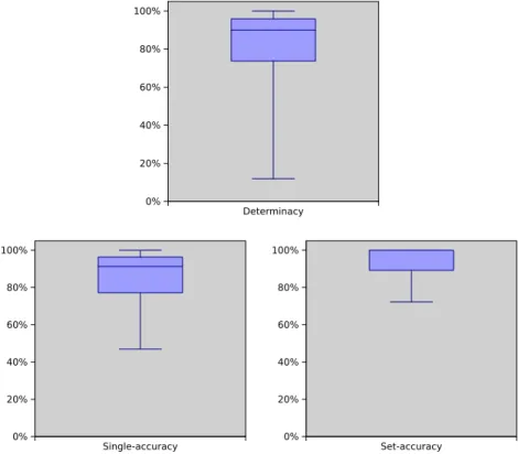
The overall performance of a credal classifier is fully characterized by four indicators, as explained in[14]: determinacy, i.e., the percentage of instances determinately classified;

single-accuracy, i.e., the accuracy on thedeterminatelyclassified instances; set-accuracy, i.e., the accuracy on theindeterminatelyclassified instances;

indeterminate output size: the average number of classes returned on the indeterminately classified instances. Note that set-accuracy and indeterminate output size are meaningful only if the data set has more than two classes.

However, how to compare a credal and a precise classifier is still an open problem. Following the approach of[14], we compare TANC and TAN by just evaluating separately the accuracy of TAN on the instances classified determinately and inde-terminately by TANC. The rationale is that, if TANC is good at separating hard-to-classify from and easy-to-classify instances, TAN should be less accurate on the instances indeterminately classified by TANC.

Instead, there are two metrics for comparing credal classifiers, which have been proposed in[16]. The first metric, bor-rowed from multi-label classification,6_{is thediscounted-accuracy:}

d-acc¼1 N XN i¼1 ðaccurateÞi jZij ;

where (accurate)iis a 0–1 variable, showing whether the classifier is accurate or not on theith instance; |Zi| is the number of

classes returned on theith instance andNis the number of instances of the test set. However, discountinglinearlythe accu-racy on the output size is arbitrary. For example, one could instead discount on |Zi|2.

The non-parametricrank testovercomes this problem. On each instance we rank two classifiers CL1and CL2as follows:

if CL1is accurate and CL2inaccurate: CL1wins;

if both classifiers are accurate but CL1returns less classes: CL1wins (the same for CL2);

if both classifiers are wrong: tie.

if both classifiers are accurate with the same output size: tie.

Fig. 3.Algorithm to compute Eq.(9).

6

We assign rank 1 to the classifier which wins, rank 2 to the classifier which looses and rank 1.5 to both classifiers in case of tie. Then, we check via the Friedman test (significance level 5%) whether the difference between the rank of the classifiers is significant. The rank test is more robust than d-acc, as it does not encode an arbitrary function for the discounting; yet, it uses less pieces of information and can therefore be less sensitive. Overall, a cross-check of the both indicators is recommended.

7.1. Overall performance of TANC

In this section, we evaluate the performance of TANC oncompletedata sets (missing data have been replaced by the mode for categorical variables, and by the average for numerical ones). On each training-test split of cross-validation, we learn the TAN structure using an algorithm (imported from the WEKA library[21]) which minimizes the MDL cost function.

InFig. 4, we present the boxplots (whose population is constituted by the results measured on 45 data sets) of three

indi-cators of performance for TANC. TANC has a quite high determinacy (median around 90%); the determinacy generally in-creases with the number of instances (large data sets reduce the importance of the prior) and dein-creases with the number of classes and features. For example, we have taken thekr–kpdata set (3196 instances) and observed monotonically increas-ing determinacy if we choose, from the 3196 instances, random subsets with 50, 100, 500 and 1000 instances to process (in-stead of all 3196 instances). The average determinacies (10 random runs for each subset size) are, respectively, 36%, 75%, 95% and 98%, which support the expected theoretical behavior of as more determinacy as more data. Using a fixed joint distri-bution generating the data, probability intervals shrink with amount of data, and so determinacy increases. Yet, the speed of increase of determinacy with data depends on the data distribution: for instance, if a data set is generated from a very skewed/uneven distribution, determinacy will increase much slower.

We have observed very low determinacy on data sets which are small and contain many classes or features; for instance, the determinacy is under 20% onaudiology(226 instances, 69 features, 24 classes),primary-tumor(339 instances, 17 features, 22 classes) andsquash-stored(52 instances, 11 features, 3 classes). Such data sets require the estimation of a considerable number of parameters (because of the amount of joint states of features and classes) with a limited sample size; yet, the learned TAN structures do not seem to be aware of this problem, as they assign a second parent (besides the class) to most features (in principle, the TAN structure can assignor nota second parent to each feature). On audiology, a conditional den-sityp(F1|f2,c) (where the pairf2,cdenotes the joint values of the parents) contains generally two parameters, estimated on

less than five instances. A similar situation is also found on the other mentioned data sets. Also the case ofoptdigits(5600 instances, 62 features, 10 classes, 10 states per feature) is interesting; despite the large size of the data set, TANC achieves a

Fig. 4.Boxplots of several performance indicators for TANC; the boxplots of determinacy and single-accuracy are computed on 45 data sets; the boxplot of set-accuracy is computed on 31 data set (the 14 binary data sets have been not considered).

determinacy of only around 57%. In fact, a generic conditional densityp(F1|f2,c) contains on average 10 parameters,

esti-mated on about 50 instances. Yet, since the features have uneven distributions, some densities are estiesti-mated on just 10– 15 samples. The joint frequencies induced in the contingency tables are numerically small, causing the indeterminacy of TANC. In a modified version of the data set, where we have made all features binary, the determinacy of TANC rises up to 98%. The reason for the indeterminacy of TANC on such data sets is therefore atoo complexTAN structure with respect to the amount of data.

The boxplots about single-accuracy and set-accuracy show that TANC is reliable (medians are about 90% and 100%, respectively). The set-accuracy is especially high, showing that indeterminate classifications do preserve the reliability of TANC on hard-to-classify instances. On average, TANC returns about 70% of the classes of the problem, when it is indeter-minate (excluding binary data sets from the computation).

7.2. TANC and TAN

We start the comparison between TANC and TAN by pointing out that the accuracy of TAN drops on average of 28 points on the instances which are indeterminately classified by TANC. InFig. 5we present a scatter plot (each point refers to a data set) of the accuracy achieved by TAN on the instances classified determinately and indeterminately by TANC. In the follow-ing, by ‘‘decrease” we mean the decrease of TAN accuracy between instances which are determinately and indeterminately classified by TANC. A very small decrease is observed onsolar-flare-X(98–96.5%); this is due to the fact that the majority class covers 98% of the instances, which can be seen as baseline for accuracy on this data set. Other data sets where the decrease is quite small include for instancesquash-unstored(93–85%) andgrub-damage(56–48%); such data sets have small number of instances with high number of classes or features; under such situations, as we have already seen, the structures are too complex and cause TANC to become excessively imprecise. Interestingly, onoptdigitsthe decrease is from 99% to 86% on the original data set, but from 94% to 47% on the binary version. Otherwise, on data sets with two classes, the accuracy of TAN on the instances indeterminately classified is comparable to random guessing or even worse (diabetes: 9%; credit: 55%,kr–kp: 40%); however, as the number of classes increases, TAN performs better on the instances indeterminately clas-sified; this might show that as the number of classes increases, as TANC is more unnecessarily indeterminate.

7.3. TANC and TANC*

Two main differences exist between TANC and TANC*_{: the model of prior ignorance (TANC adopts the EDM, while TANC}*

the local IDM) and the treatment of missing data (TANC*_{assumes MAR, while TANC assumes nonMAR). We focus on}

assess-ing the impact of the model of prior ignorance; to remove the effect of missassess-ing data, we work oncompletedata sets. We did not implement TANC*_{in our code; rather, we have compared our results with those published in[15]; although the}

compar-ison has to be taken with some cautiousness, the results underlie clear patterns which allow us to draw some conclusions. We consider the six complete data sets analyzed in[15]. TANC is more determinate than TANC*_{, as it can be seen from}

Fig. 6; on average, the increase of determinacy is of 19 points percentile. This is the result of the smaller credal set built

by the EDM compared to the local IDM. However, the determinacy of the two classifiers is equivalent onkr–kp(around 3200 instances, only binary features), where the role of the prior is not influential.

Moreover, from the indicators reported in[15], we build an approximate estimate of the discounted-accuracy of TANC*_{, as}

follows:

d-accdetermsingleAccþsetAcc ð1detÞ

ðindOutSzÞ ð10Þ

where the first term is the contribution to d-acc coming from determinately classified instances, and the second term is the contribution from indeterminately classified ones. The approximation lies in the fact that, for the indeterminately classified instances, we divide theaverageaccuracy byindOutSz, which is theaverageoutput size, instead of dividing accuracy and out-put size instance by instance and averaging only at the end over all the instances.

The d-acc (computed in the approximated way for both classifiers, to provide a fair comparison) are shown inFig. 6; TANC outperforms sensibly TANC*_{in all data sets, apart fromkr–kp, where both classifiers perform the same.}

7.4. TANC vs. NCC

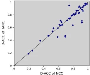
Overall, TANC is slightly inferior to NCC, as shown by the scatter plot of the discounted accuracies of the two classifiers

(Fig. 7). The rank test returns 30 ties, 9 wins for NCC and 6 wins for TANC. The data sets where the rank test returns a victory

of NCC include some data sets where the Bayesian TAN is outperformed by NBC (for instance, the already mentionedlabor, contact-lenses, pasture) and which are in general quite small; however, they also include some further data sets where TAN is as good as, or even better than, NBC. A striking example is the already mentionedoptdigits: here TAN is slightly better than NBC; their average accuracies are 94% and 92%. On this data set, NCC has determinacy 96%, and d-acc of 0.91; on the other hand, TANC has determinacy only of 57% (the reasons have been already analyzed), achieving a d-acc of 67%. The same pat-tern (lower d-acc of TANC due to much lower determinacy than NCC) is observed for instance also onlymph.

On the other hand, TANC outperforms NCC on data sets which include correlated variables; for instance,kr–kp,vowel,

monks-1. Moreover, TANC outperforms NCC on the binary version of optdigits.

We recognize that the current implementation of TANC is generally less effective than NCC (although in a few examples it does outperform NCC), although the Bayesian TAN is generally more accurate than NBC. As already explained, the problem lies in the learned TAN structures, which should be simpler (i.e., contain less dependencies) to be better suited for a classifier based on imprecise probabilities. Currently, to our knowledge there are no structure learning methods that are specially de-signed for credal networks.

Fig. 6.TANC vs. TANC*

.

7.5. Preliminary results with missing data

In this section, we compare the determinacy and the accuracy of TANC and NCC (in its updated version that is able to deal with nonMAR missing data[14]) in the presence of missing data. We recall that by nonMAR we indicate ignorance about the MP, which also implies that MAR cannot be assumed. We consider four data sets, whose characteristics are described in the first four column ofTable 2. We considered the complete data sets and then artificially generate missing values by using a selective MP that targeted only certain values of the features, that is, for a given feature, we have randomly selected one of its categories and then removed (at random over the instances that contained that category) some of them. Such procedure leads to nonMAR missing data. The data are divided into training and testing sets with a 2/3 split (testing set is complete as we only generate missing values in the training data).

As shown inTable 2, the determinacy of TANC is constantly inferior to that of NCC, and decreases drastically in thevote

data set. In particular, this data set contains several instances where two features, which are interconnected in the TAN structure, are missing at the same time; this can explain the higher determinacy of NCC compared to TANC. On the other hand, the discounted-accuracy of TANC in the very same data set remains equivalent to that of NCC, which shows that TANC was more accurate on deciding which instances are harder (or easier) to classify. In fact, using thevotedata set, TANC has 98.63% of accuracy when it returns a single class, while NCC achieves only 70%. TANC is also more accurate when answering a single class onbreast-wandcrx(in thesoybeandata set, none of them ever answered a single class). This observation can also be concluded from the fact that TANC was slightly less determinate in all data sets, yet keeping the d-acc at the same level. TANC achieves slightly better results in thecrxdata set, slightly worse results in thesoybean

data set, and mostly the same accuracy inbreast-wandvote. As already discussed in this section, data sets likesoybean

with many classes and features (when compared to the amount of data) are more susceptible to indeterminate classifications.

8. Conclusions

TANC is a new credal classifier based on a tree-augmented naive structure; it treats missing data conservatively by con-sidering all possible completions of the training set, but avoiding an exponential increase of the computational time. TANC adopts the EDM as a model of prior ignorance; we have shown that EDM is a reliable and computationally affordable model of prior near-ignorance for credal classifiers. We have shown that TANC is more reliable than precise TAN (learned with uni-form prior) and that it obtains better peruni-formance compared to a previous TAN model based on imprecise probabilities, but learned with a local IDM approach; the adoption of EDM overcomes the problem of the unnecessary imprecision induced by the local IDM, while keeping the computation affordable.

TANC has shown good accuracy when compared to NCC, but overall is still behind NCC’s performance. One main reason for such results lies on the algorithm to learn the TAN structure. Finding the best TAN structure is a challeng-ing problem, and has strong impact even for precise classifier. In the case of credal classifiers such as TANC, the struc-ture must be learned accordingly, that is, the strucstruc-ture learning method must take into account the imprecise nastruc-ture of the classifier to build the best structure for such model. Our experiments indicate that a more cautious structure with respect to that learned for a precise classifier might obtain better performance in the credal version. Unfortu-nately, learning the structure of a credal network is a hard problem currently without practical solutions, and we were forced to learn the structure using a standard method that does not take the credal nature of the model into account.

The TANC classifier has room for many improvements. The treatment of MAR and nonMAR missing data all together, appearing both in the training and the testing set are the main topics for future work. In order to make TANC less indeter-minate on incomplete data sets, a solution could be to allow for mixed configurations, in which some features are treated as MAR and some others are not. This would allow both for a decrease of indeterminacy and for a finer-grained tuning of the way that missing data are dealt with. Besides that, the computational performance of TANC can also be further improved, for example, with the use of dynamic programming. Extensions beyond trees are also of interest, but they fall into the need of fast and accurate inference methods for general credal networks.

A further open problem, of interest in general for credal classification, is the development of metrics to compare credal classifier and classifiers based on traditional probability.

Table 2

Comparison of TANC and NCC in a few data sets with missing data.

Number of Determinacy (%) D-ACC (%)

Data set Feats Inst. Classes Missing TANC NCC TANC NCC

breast-w 9 350 2 8 97.4 99.4 96.1 96.8

crx 15 345 2 54 84.9 90.1 85.2 84.9

soybean 35 290 19 128 00.0 00.0 13.9 15.7

Acknowledgement

Work partially supported by the Swiss NSF Grants Nos. 200021-118071/1 and 200020-116674/1 and by the projectTicino in rete.

Appendix A. Correctness of the algorithm for dominance test

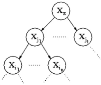
This section describes the details and correctness of the algorithm to compute the value of the dominance test (Fig. 3). The idea of the algorithm to evaluate Eq.(9)is to combine the computations that are performed separately in the children of each variable and then to propagate the best possible solution to their sole parent. We ignore the arcs fromCbecause we look for

pðyjc1Þ ¼mindc1

Ypðyjc1Þand

pðyjc2Þ ¼maxdc2

Ypðyjc2Þ, that is, the actual root variableCis observed. The computation starts on

the leaves and follows in a bottom-up idea. At each variableXi, the goal is to obtain the joint probabilityp(yr(i)|yi,c) of its

descendants conditional onyi7(cequalsc1orc2depending whether it is the minimization or the maximization). This

evalu-ation is done for all possible completionsdc1

Xiand it is optimized over the completions of the children. The result is stored in a

cache/_iðdc1

XiÞ.Fig. A.8shows part of a network. AtXj1, the joint probabilitiespðyrðikÞjyik;cÞof every childXik2Kj1 (for every pos-sible completion of that sub-tree) are already computed. So, they are combined to obtainpðy_rðj1Þjyj1;cÞ, for every possible com-pletion ofXj1. We perform such idea for eachj1,. . .,jt, obtaining the probabilitiespðyrðj1Þjyj1;cÞ;. . .;pðyrðjtÞjyjt;cÞthat are then

made available to the parentXp, where the computations are analogous but using the information obtained fromXj1 and its siblings. The process goes through the tree structure until reaching the root.

Suppose that the root variables (ifCis not considered) areX1,. . .,Xr. So,

pðyjc1Þ ¼ Yr j¼1 pðyjjc1Þ pðyrðjÞjyj;c1Þ ¼Y r j¼1 pðyjjc1Þ Y Xi2Kj pðyijyj;c1ÞpðyrðiÞjyi;c1Þ 0 @ 1 A; and, in general min dc1 Y pðyrðjÞjyj;c1Þ ¼min dc1 Y Y Xi2Kj pðyijyj;c1ÞpðyrðiÞjyj;c1Þ 0 @ 1 A: ðA1Þ

Now, when we complete the variableXj, the childrenKjhave separable computations. They are separable because the

countsnthat appear in the children ofXjare independent of each other as they concern disjoint subsets of variables (the

structure is a tree, soXrðiÞ\Xrði0_Þ¼ ;forXi;X_i02K_j, withi–i0andXj¼Pi¼Pi0.). The only dependent value isn_c

1yj, as it

ap-pears in the denominators of distinct children ofXj(it appears in the denominator of the estimation of eachp(yi|yj,c1) in Eq. (A1)). However,nc1yjis fixed as the problem is solved for every possible completion ofXj. Besides that, note that the terms

a

are not present in this formulation because we treat them using the hidden missing instance. Hence, the overall computation can be decomposed as min dc1 Xj;X_rðjÞ pðyrðjÞjyj;c1Þ ¼min dc1 Xj;Xi Y Xi2Kj pðyijyj;c1Þ min dc1 Xi;X_rðiÞ pðyrðiÞjyi;c1Þ 0 @ 1 A;

which is solved for each completion ofXjin a recursive formulation: for alldcX1j,

/j d c1 Xj ¼min dc1 Xi Y Xi2Kj pðyijyj;c1Þ min dc1 Xi;X_rðiÞ pðyrðiÞjyi;c1Þ 0 @ 1 A; ¼ Y Xi2Kj min dc1 Xi pðyijyj;c1Þ /i d c1 Xi ;¼ Y Xi2Kj min dc1 Xi nc1yiyj nc1yj /i d c1 Xi ! ; ðA2Þ

Fig. A.8. Part of the computation tree of the TANC algorithm.

7

where/jðd c1

XjÞis assumed to be equal to one ifXjis a leaf. The maximization is analogous. An important fact in Eq.(A2)is that

it is enough to keep the best possible solution for every completion of a variable without having to record all the completions of its descendants. This is valid becausenc1yiyjis known when the completiond

c1

Xiis given (nc1yjwas already fixed by the

com-pletion ofXj), so completions of variables inXr(i)are irrelevant for the minimization in Eq.(A2), and it is enough to have the

best possible solution of the children/i() for eachdcX1i.

Because of that, the algorithm is implemented in a bottom-up manner so as the/’s of children are available when a given variable is treated, which reduces the complexity of the method to be exponential in the number of missing values of only two variables (a variable and its parent) instead of all missing values. It is worth mentioning that in the last step of the algo-rithm, all the values/_iðdc1

XiÞare computed for each variableXi,i6r, that has only the class as parent. Finally, we obtain Table B.3

Detailed results data set by data set of TANC and TANC (first 22 data sets). TAN-P and TAN-I indicate the accuracy of the Bayesian TAN when TANC is, respectively, determinate and indeterminate. Moreover,Nfdenotes the number of features,nis the number of instances andNcis the number of classes.

Data set Nf n Nc TANCC performance TAN

Det. (%) Sg-Acc (%) SetAcc (%) Ind.Sz. Tan-P (%) Tan-I (%)

audiology 69 226 24 11.9 98.1 98.0 14.1 98.1 70.7 breast-w 9 683 2 98.1 97.8 100.0 2.0 97.8 86.1 cmc 9 1473 3 91.5 55.2 81.2 2.1 55.2 35.8 contact-lenses 4 24 3 41.7 100.0 100.0 2.7 100.0 58.3 credit 15 1000 2 91.3 76.1 100.0 2.0 76.1 46.3 credit-a 15 690 2 96.1 88.1 100.0 2.0 88.1 42.0 diabetes 6 768 2 98.6 79.1 100.0 2.0 79.1 53.3 ecoli 6 336 8 91.1 85.8 91.7 3.9 85.8 43.7 eucalyptus 17 736 5 77.9 65.0 80.2 2.3 65.0 48.0 glass 7 214 7 73.9 76.1 87.6 3.6 76.1 50.3 grub-damage 8 155 4 58.7 56.2 86.4 2.4 56.2 48.3 haberman 3 306 2 95.8 75.4 100.0 2.0 75.4 21.4 heart-c 11 303 5 25.5 96.2 80.5 4.1 96.2 76.5 heart-h 9 294 5 73.3 89.3 83.4 4.1 89.3 69.7 hepatitis 17 155 2 91.5 85.9 100.0 2.0 85.9 95.8 iris 4 150 3 98.7 94.6 100.0 2.5 94.6 50.0 kr–kp 36 3196 2 99.0 92.5 100.0 2.0 92.5 56.1 labor 11 57 2 75.3 97.5 100.0 2.0 97.5 70.8

liver-disorders 1 345 2 100.0 63.2 n.a. n.a. 63.2 n.a.

lymph 18 148 4 17.9 93.6 91.3 2.6 93.6 81.2

monks-1 6 556 2 100.0 94.6 n.a. n.a. 94.6 n.a.

monks-2 6 601 2 96.0 64.8 100.0 2.0 64.8 47.2

monks-3 6 554 2 99.6 98.0 100.0 2.0 98.0 0.0

Table B.4

Detailed results data set by data set of TANC and TAN (last 23 data sets). TAN-P and TAN-I indicate the accuracy of the Bayesian TAN when TANC is, respectively, determinate and indeterminate. Moreover,Nfdenotes the number of features,nis the number of instances andNcis the number of classes.

Data set Nf n Nc TANCC performance TAN

Det. (%) Sg-Acc (%) SetAcc (%) Ind.Sz. Tan-P (%) Tan-I (%)

nursery 8 12960 5 94.1 93.8 80.6 2.0 93.7 71.1 optdigits 62 5620 10 57.2 99.9 99.7 5.6 99.9 87.0 optdgtBinary 63 5620 10 97.9 94.3 80.5 2.2 94.3 47.2 pasture 10 36 3 76.0 96.7 100.0 2.6 96.7 35.7 primary-tumor 17 339 22 14.9 67.9 67.3 9.1 67.9 43.9 segment 7 810 7 93.9 95.1 98.0 2.5 95.1 62.7 sol-flare_C 10 323 3 81.1 90.0 90.7 2.3 90.0 87.6 sol-flare_M 10 323 4 69.1 93.2 75.9 2.6 93.2 69.6 sol-flare_X 10 323 2 80.6 97.5 100.0 2.0 98.2 96.4 sonar 21 208 2 89.0 90.9 100.0 2.0 90.9 64.6 spect 22 267 2 87.7 83.3 100.0 2.0 83.3 68.3 splice 34 3190 3 95.8 97.2 99.6 2.1 97.2 73.1 squash-st 11 52 3 15.2 91.7 100.0 2.7 91.7 75.0 squash-unst 14 52 3 14.9 92.9 100.0 2.7 92.9 85.2

tae 2 151 3 100.0 47.0 n.a. n.a. 47.0 n.a.

vehicle 18 846 4 82.4 77.6 89.1 2.3 77.6 49.1 vowel 13 990 11 76.4 78.1 89.3 2.7 78.1 54.7 waveform 19 5000 3 92.0 83.9 99.6 2.0 83.9 64.5 wine 13 178 3 94.4 100.0 100.0 2.2 100.0 66.7 yeast 7 1484 10 95.5 60.5 72.3 3.1 60.5 29.1 zoo 16 101 7 74.8 100.0 100.0 3.6 100.0 88.0

pðyjc1Þ ¼/CðÞ ¼ Y Xi2KC min dc1 Xi nc1yi nc1 /i d c1 Xi ; ðA3Þ

and similarly for the maximization. This final step returns the desired valuespðyjc2Þandp(y|c1), which are later multiplied by p(c2) andp(c1), respectively, to obtain the value of the dominance test.

Appendix B. Detailed results data set by data set Tables B.3, B.4, B.5, B.6

Table B.5

Comparison of TANC and NCC data set by data set (first 22 data sets). Det denotes determinacy and d-acc denotes discounted-accuracy. Moreover,Nfdenotes

the number of features,nis the number of instances andNcis the number of classes.

Data set Nf n Nc TANC NCC RankTest

Det. (%) D-acc Det. (%) D-acc

audiology 69 226 24 11.9 0.24 9.8 0.25 NCC breast-w 9 683 2 98.1 0.97 100.0 0.98 TIE cmc 9 1473 3 91.5 0.54 96.5 0.52 TIE contact-lenses 4 24 3 41.7 0.64 66.7 0.80 NCC credit 15 1000 2 91.3 0.74 96.9 0.75 TIE credit-a 15 690 2 96.1 0.87 98.3 0.87 TIE diabetes 6 768 2 98.6 0.79 99.7 0.78 TIE ecoli 6 336 8 91.1 0.81 92.2 0.83 TIE eucalyptus 17 736 5 77.9 0.59 75.5 0.53 TANC glass 7 214 7 73.9 0.64 72.4 0.65 TIE grub-damage 8 155 4 58.7 0.47 58.7 0.47 TIE haberman 3 306 2 95.8 0.74 95.8 0.74 TIE heart-c 11 303 5 25.5 0.39 20.4 0.35 TIE heart-h 9 294 5 73.3 0.71 77.5 0.72 TIE hepatitis 17 155 2 91.5 0.83 94.8 0.84 TIE iris 4 150 3 98.7 0.94 98.0 0.94 TIE kr–kp 36 3196 2 99.0 0.92 98.8 0.88 TANC labor 11 57 2 75.3 0.86 90.0 0.93 NCC liver-disorders 1 345 2 100.0 0.63 100.0 0.63 TIE lymph 18 148 4 17.9 0.47 58.2 0.69 NCC monks-1 6 556 2 100.0 0.95 100.0 0.75 TANC monks-2 6 601 2 96.0 0.64 96.7 0.61 TIE monks-3 6 554 2 99.6 0.98 100.0 0.96 TIE Table B.6

Comparison of TANC and NCC data set by data set (last 23 data sets). Det denotes determinacy and d-acc denotes discounted-accuracy. Moreover,Nfdenotes the

number of features,nis the number of instances andNcis the number of classes.

Data set Nf n Nc TANC NCC RankTest

Det. (%) D-acc Det. (%) D-acc

nursery 8 12960 5 94.1 0.91 99.7 0.90 TIE optdigits 62 5620 10 57.2 0.68 96.1 0.92 NCC optdgtBinary 63 5620 10 97.9 0.93 98.8 0.89 TANC pasture 10 36 3 76.0 0.82 81.7 0.88 TIE primary-tumor 17 339 22 14.9 0.19 10.7 0.20 TIE segment 7 810 7 93.9 0.92 95.7 0.93 TIE sol-flare_C 10 323 3 81.1 0.80 85.4 0.81 TIE sol-flare_M 10 323 4 69.1 0.75 71.1 0.76 TIE sol-flare_X 10 323 2 80.6 0.88 93.2 0.92 TIE sonar 21 208 2 89.0 0.86 96.6 0.84 TIE spect 22 267 2 87.7 0.79 95.2 0.79 TIE splice 34 3190 3 95.8 0.95 99.1 0.96 TIE squash-st 11 52 3 15.2 0.45 46.8 0.59 NCC squash-unst 14 52 3 14.9 0.45 46.9 0.69 NCC tae 2 151 3 100.0 0.47 92.7 0.46 TIE vehicle 18 846 4 82.4 0.71 93.3 0.63 TANC vowel 13 990 11 76.4 0.68 76.6 0.64 TANC waveform 19 5000 3 92.0 0.81 99.3 0.81 TIE wine 13 178 3 94.4 0.97 97.8 0.99 TIE yeast 7 1484 10 95.5 0.59 97.0 0.59 TIE zoo 16 101 7 74.8 0.83 80.6 0.88 NCC

References

[1] P. Domingos, M. Pazzani, On the optimality of the simple Bayesian classifier under zero-one loss, Machine Learning 29 (2/3) (1997) 103–130. [2] D. Hand, K. Yu, Idiot’s bayes-not so stupid after all?, International Statistical Review 69 (3) (2001) 385–398

[3] J. Friedman, On bias, variance, 0/1 – loss, and the curse-of-dimensionality, Data Mining and Knowledge Discovery 1 (1997) 55–77.

[4] R. Kohavi, Scaling up the accuracy of naive-Bayes classifiers: a decision-tree hybrid, in: Proceedings of the Second International Conference on Knowledge Discovery and Data Mining, AAAI Press, 1996, pp. 202–207.

[5] N. Friedman, D. Geiger, M. Goldszmidt, Bayesian network classifiers, Machine Learning 29 (2) (1997) 131–163.

[6] M. Madden, On the classification performance of TAN and general Bayesian networks, Knowledge-based Systems 22 (7) (2009) 489–495. [7] P. Walley, Statistical Reasoning with Imprecise Probabilities, Chapman and Hall, New York, 1991.

[8] J.-M. Bernard, An introduction to the imprecise Dirichlet model for multinomial data, International Journal of Approximate Reasoning 39 (2–3) (2005) 123–150.

[9] M. Zaffalon, Statistical inference of the naive credal classifier, in: G. de Cooman, T.L. Fine, T. Seidenfeld (Eds.), ISIPTA ’01: Proceedings of the Second International Symposium on Imprecise Probabilities and their Applications, Shaker, The Netherlands, 2001, pp. 384–393.

[10] A. Cano, M. Gómez-Olmedo, S. Moral, Credal nets with probabilities estimated with an extreme imprecise Dirichlet model, in: ISIPTA ’07: Proceedings of the Fourth International Symposium on Imprecise Probabilities and their Applications, SIPTA, Prague, 2007, pp. 57–66.

[11] R.J.A. Little, D.B. Rubin, Statistical Analysis with Missing Data, Wiley, New York, 1987.

[12] M. Zaffalon, Exact credal treatment of missing data, Journal of Statistical Planning and Inference 105 (1) (2002) 105–122.

[13] M. Zaffalon, Conservative rules for predictive inference with incomplete data, in: F.G. Cozman, R. Nau, T. Seidenfeld (Eds.), ISIPTA ’05: Proceedings of the Fourth International Symposium on Imprecise Probabilities and their Applications, SIPTA, Manno, Switzerland, 2005, pp. 406–415.

[14] G. Corani, M. Zaffalon, Learning reliable classifiers from small or incomplete data sets: the naive credal classifier 2, Journal of Machine Learning Research 9 (2008) 581–621.

[15] M. Zaffalon, E. Fagiuoli, Tree-based credal networks for classification, Reliable Computing 9 (6) (2003) 487–509.

[16] G. Corani, M. Zaffalon, Lazy naive credal classifier, in: Proceedings of the First ACM SIGKDD Workshop on Knowledge Discovery from Uncertain Data, ACM, 2009, pp. 30–37.

[17] G. Corani, M. Zaffalon, JNCC2: the java implementation of naive credal classifier 2, Journal of Machine Learning Research 9 (2008) 2695–2698. [18] A. Asuncion, D. Newman, UCI machine learning repository, 2007. Available from:<http://www.ics.uci.edu/mlearn/MLRepository.html>.

[19] U.M. Fayyad, K.B. Irani, Multi-interval discretization of continuous-valued attributes for classification learning, in: Proceedings of the 13th International Joint Conference on Artificial Intelligence, Morgan Kaufmann, San Francisco, CA, 1993, pp. 1022–1027.

[20] G. Tsoumakas, I. Vlahavas, Random k-labelsets: an ensemble method for multilabel classification, in: Proceedings of the 18th European conference on Machine Learning, Springer-Verlag Berlin, Heidelberg, 2007, pp. 406–417.