Energy Procedia 14 (2012) 1883 – 1888
1876-6102 © 2011 Published by Elsevier Ltd. Selection and/or peer-review under responsibility of the organizing committee of 2nd International Conference on Advances in Energy Engineering (ICAEE).
doi:10.1016/j.egypro.2011.12.887
Energy
Procedia
Energy Procedia 00 (2011) 000–000www.elsevier.com/locate/procedia
Application of Artificial Neural Networks and Fuzzy logic
Methods for Short Term Load Forecasting
A. Badri, Z. Ameli, A.Motie Birjandi
Shahid Rajayee Teacher Training University, Lavizan, Tehran, Iran
Abstract
Accurate load forecasting is a great help for electric companies to make the best decisions in terms of unit commitment, generation and maintenance planning, etc. It is necessary that electric generation companies have prior knowledge of future demand with great accuracy. Some data mining algorithms play the greater role to predict the load forecasting. This paper investigates the application of artificial neural networks (ANN) and fuzzy logic (FL) as forecasting tools for predicting the load demand in short term category. In this case the forecasting is day ahead and it is observed that ANN represents the more accurate results in comparison to FL. Finally application of ANN in medium term load forecasting is implemented and the results are compared.
© 2011 Published by Elsevier Ltd.
Keywords: Load forecasting, Artificial neural networks, Fuzzy logic
1. Introduction
Accurate load forecast (LF) provides system dispatchers with timely information to operate the system economically and reliably. It is also necessary because availability of electricity is one of the most important factors for industrial development [1]. Traditional approaches to forecast energy demand explain relationships between observable variables and the desired parameter to be forecasted. Researchers have used many variables as input independent variables for load forecasting. They consist of number of customers, number of high temperature days, total housing units, cost of fuel, average temperature, number of population, per capita personal income, and percent rural population [2]. While some of the models are easy to perform when data are available, other models are complex and difficult to understand and apply. Some researches depend on the availability of associated data.
Most of these models are used for long-term planning [3]. Most forecasting methods use statistical techniques or artificial intelligence algorithms such as regression, artificial neural networks (ANN), fuzzy logic (FL), and expert systems. Two of the methods, so-called end-use and econometric approach are broadly used for medium- and long-term forecasting. A variety of methods, such as various regression models, time series, artificial neural networks, statistical learning algorithms, fuzzy logic, and expert systems, have been developed for short-term forecasting [4]. In recent years, many researches have been carried out on the application of artificial neural network techniques and fuzzy logic to the load forecasting problem. Expert systems have been tried out and compared to traditional methods [5]. Among various methods applied for LF, ANN and FL are the most popular and commonly tools for LF © 2011 Published by Elsevier Ltd. Selection and/or peer-review under responsibility of the organizing committee of 2nd International Conference on Advances in Energy Engineering (ICAEE).Open access under CC BY-NC-ND license.
applications. Load forecasting depends on operating time horizon of load occurrence. Accordingly, load forecasting is classified in three categories such as short term load forecasting, medium term load forecasting, and long term load forecasting [6]. Short term load forecast is applicable for load forecasts within one day to one week ahead of load occurrence, while medium term load forecast is applicable for forecasting loads in a period within one week to one month ahead of load occurrence. For each classification there are appropriate methods for load forecasting. Here, we are going to show the impact of ANN and FL in short term load forecasting. This paper attempts to compare two new techniques for short term load forecasting. The paper is organized as follows: In sections 2 and 3 the mathematical models for short term load forecasting with FL and ANN are proposed. In section 4 a case study to show the application of two methods is represented and compare between short-term and medium-term LF with ANN, finally in section 5 provided the conclusion.
2. Short Term Load Forecasting with Fuzzy Logic Systems:
Fuzzy Logic has proposed in several papers for short term load forecasting [7]. For the proof of the method a fuzzy expert system that forecasts the daily peak load, is selected. Sometimes it is necessary to have crisp output. With such crisp inputs and outputs, a fuzzy expert system implements a non-linear mapping from the input space to the output space. This mapping is done by a number of if-then rules, each of which describes a local behavior of the mapping.
To illustrate this is considered:
X: a set of data or objects. (i.e. Forecast temperature values), A: Another set containing data (or objects), x: An individual value of the data set and μA (x) is the membership function that connects the
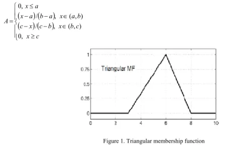
set X and A.μA (x) determines the degree that x belongs to A. Its value varies between 0 and 1. The membership function is selected by trial and error. There are four basic membership functions
namely: Triangular, Trapezoidal, Gaussian, Generalized bell [7]. In general, we would like to choose the membership functions which overlap with other neighboring membership functions by 25-30 %. In addition, we would like to select reasonable membership values [8]. In this paper triangular function is chosen because this function is simple and most frequently used.The triangular function is defined as that have three parameters 'a' (minimum), 'b' (middle) and 'c' (maximum) that determine the shape of the triangle. Figure 1 shows the triangular function
(1)
Figure 1. Triangular membership function 3. Short Term Load Forecasting with Artificial neural network:
(
) (
)
(
) (
)
⎪ ⎪ ⎩ ⎪ ⎪ ⎨ ⎧ ≥ ∈ − − ∈ − − ≤ = c x c b x b c x c b a x a b a x a x A , 0 ) , ( , / ) , ( , / , 0Here, a widely used model called the multi-layered perceptron (MLP) ANN (Figure. 2) is employed. The MLP type ANN consists of one input layer, one or more hidden layers and one output layer [9].
Figure 2. Structure of a Three-Layered Perceptron type ANN
In our study input layers are in terms of load amount and temperature and output layer is estimated load amount. In architecture of MLP type ANN each layer employs various neurons and each neuron in a layer is connected to the neurons in the adjacent layer with different weights. Signals flow into the input layer, pass through the hidden layers, and arrive at the output layer. With the exception of the input layer, each neuron receives signals from the neurons of the previous layer linearly weighted by the interconnect values between neurons. The neuron then produces its output signal by passing the summed signal through a sigmoid function. In this paper, the generalized delta rule (GDR) is used to train a layered perceptron-type ANN.
A total of Q set of training data are assumed to the available. Inputs of {
i
1,
i
2,
i
3,...,
,
i
Q} are imposed on the top layer. The ANN is trained to respond to the corresponding target vectors,{t
1,
t
2,
t
3,...,
t
Q}on the bottom layer. The output from neuron I,Oi, is connected to the input of neuron j through the interconnection weight Wij. The state of the neuron k is:(2) Where
f
(
x
)
=
1
(
1
+
e
−x)
and sum of all neurons in the adjacent layer. Let the target state of the output neuron be t. thus the error at the output neuron can be defined as:(3) Where neuron k is the output neuron. according to the difference between the produced and target outputs, the network’s weights {Wij} are adjusted to reduce the output error. The error at the output layer propagates backward to the hidden layer, until it reaches the input layer[10]
The GRD algorithm adapts the weights according to the gradient error, i.e:
(4) To evaluate the result of ANN performance, the following percentage error measure is employed.
(5)
4. Case Study
In order to implement a short term load forecasting a 24 hours load data is considered as shown in Table. I. As illustrated for each hour the load amount and corresponding temperature are provided. These are used as input data for ANN training and for inputs of proposed fuzzy logic approach as well.
100 × − = load actual load forecasted load actual error ij j j ij ij W O O E W E W ∂ ∂ ∂ ∂ − = ∂ ∂ − Δ α ) ( i i ik k f W O O =
∑
2)
(
2
1
k kO
t
E
=
−
18 20 22 24 26 28 30 1800 2000 2200 2400 2600 2800 3000 Temperature P eak Loa d
Polynomial Curve Fitting On Data Table I. data of load and temperature
Load Temperature Load Temperature Load Temperature 2194 29 2157 24 2759 26 2438 22 2780 29 2016 23 1798 23 2461 21 2908 22 1770 19 2415 23 2155 27 2390 23 2893 24 1955 28 2713 27 2071 25 2026 25 2915 26 2685 21 2501 29 1869 21 2680 27 2315 22
In order to apply fuzzy logic approach for short term LF, it is needed to have a mathematical model of actual data, in advance. It is obtained by curve fitting. As shown in Figure. 3 a straight line is fitted for these data.
Figure 3: load- temperature curve for load forecasting with FL method
Data are fitted by a linear regression curve. The actual data points are spread over the regression curve. This regression curve is calculated using MATLAB. The result of this regression analysis results in the equation of a straight line:
(6) Lp: Peak load
Tp: Forecast maximum daily temperature.
gp , hp: Constants derived from the least square based regression analysis
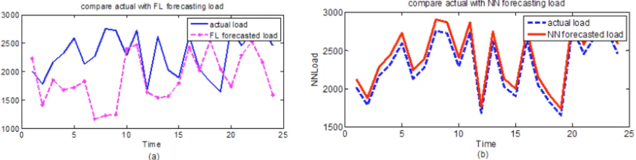
Using proposed models for FL and ANN based forecasting approaches Figure 4 shows result of the obtained hourly forecasted loads versus their corresponding actual amounts:
Figure 4: (a) Actual load data versus predicted load obtained from FL approach (b) Actual load data versus predicted load obtained from ANN approach
p p p
p
g
T
h
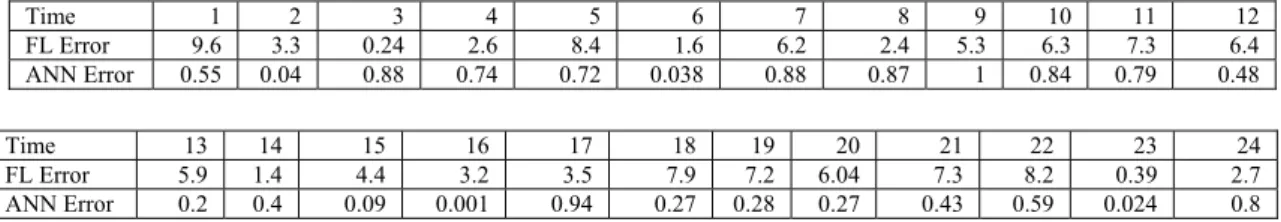
Accordingly, Table II shows the error (%) of proposed load forecasting models. As shown ANN method results in profound small errors for LF purpose in comparison to FL as the average error for ANN method is 0.5 % while for FL method is 4.91 % that is considerable.
Table II: error(%) of peak load forecasting with FL and ANN method
Time 1 2 3 4 5 6 7 8 9 10 11 12 FL Error 9.6 3.3 0.24 2.6 8.4 1.6 6.2 2.4 5.3 6.3 7.3 6.4 ANN Error 0.55 0.04 0.88 0.74 0.72 0.038 0.88 0.87 1 0.84 0.79 0.48 Time 13 14 15 16 17 18 19 20 21 22 23 24 FL Error 5.9 1.4 4.4 3.2 3.5 7.9 7.2 6.04 7.3 8.2 0.39 2.7 ANN Error 0.2 0.4 0.09 0.001 0.94 0.27 0.28 0.27 0.43 0.59 0.024 0.8
General problem with FL approach is inaccuracy of prediction and numerical instability. This is due to the fact that with the same parameters this is difficult to find an accurate and comprehensive linear regression curve for FL method. This model will not be systematically tested and the results of the tests are not presented in an entirely satisfactory manner [11]. On the contrary, ANN considers load temperature during load forecasting. With ANN one can model complex and nonlinear relationships between a training process and historical data.
In order to show the application of ANN in implementing medium-term load forecasting a six days load forecasting study is considered. In this case five set input data for six different days are considered as illustrated in Table III. Similarly, Table IV shows obtained error (%) for medium-term LF.
Here, the average error would be 1.72% that is comparable with is 0.5 % obtained from short-term LF. In fact it was expected since short-term LF based on more accurate data obtained from 24 hours ahead of load occurrence, while medium LF is based on week ahead data that are more probabilistic.
Table III: data of medium-term load forecasting Table IV: Error(%) of medium-term load forecasting
Conclusion
This paper provides a comparative study that has been carried out between two modern methods, ANN and FL for short term load forecasting. The simulation results clearly show that the ANN model produces significantly better results than FL method. This is due to the fact that with the same parameters this is difficult to find an accurate and comprehensive linear regression curve for FL method. This model will not be systematically tested and the results of the tests are not presented in an entirely satisfactory manner. As another study the application of ANN for medium-term load forecasting was presented. Due
Set1 Set2 Set3 Set4 Set5 Day1 2229 2063 1930 2461 1638 Day2 2361 2124 2291 2086 2588 Day3 2903 2076 2319 2209 2114 Day4 2220 2841 2940 1705 2482 Day5 2722 2530 1852 2624 1827 Day6 1827 2460 2802 2000 1954 Average 2100.5 2180.83 2355.67 2349.5 2377
Set1 Set2 Set3 Set4 Set5 Day1 0.5 0.32 3.1 1.15 0.4 Day2 1.4 1.9 1.7 0.8 0.9 Day3 2.87 1.09 3.6 0.9 1.9 Day4 1.65 1.6 5.2 1.75 2.5 Day5 1.04 0.86 3.8 0.63 0.21 Day6 1.89 1.6 2.8 1.8 1.7 Average 1.56 1.23 3.37 1.17 1.27
to accuracy of short-term load data and its proximity to load occurrence time, short-term LF provides more accurate results in comparison to medium-term LF. In order to have even better results, we may need to have more sophisticated topology for the neural network which can discriminate start-up days from other days. Here, we utilized only temperature among other weather information. Nevertheless, ANN may enable us to model such weather information for short term LF procedure. Use of additional weather variables such as cloud coverage and wind speed should yield even better result.
References
[1] Pradeepta Kumar Sarangi, Nanhay Singh, R. K. Chauhan and Raghuraj Singh. Short term Load Forecasting using Artifical Neural Network:A Comparison With Genetic Algoritm Implemention. ARPN Journal of Engineering and Applied Sciences; VOL. 4, NO. 9, NOVEMBER 2009
[2] Rashid Mohammed Roken, Masood A. Badri. Time Series Models for Forecasting Monthly Electricity Peak Load for Dubai. Chancellor’s Undergraduate Research Award; 2006
[3] Amit Jain, B. Satish. Clustering based Short Term Load Forecasting using Support Vector Machines, roceedings of 2009 IEEE Bucharest PowerTech conference; IIIT/TR/2009
[4] Eugene A. Feinberg, Dora Genethliou. Load Forecasting, chapter 12; 2004
[5] K.Sub Barayan, R.R. Shoults, M.T. Manry, C. KwAN. Comparison of Very Short-Term Load Forecasting Techniques, IEEE Transactions on Power Systems; 2. May 1996
[6] Badran, H. El-Zayyat and G. Halasa. Short-Term and Medium-Term Load Forecasting for Jordan's Power System. American Journal of Applied Sciences; 5 (7): 763-768, 2008
[7] R.M.Holrnukhea, Sunita Dhumaieb, P.S. Chaudhari. Short Term Load Forecasting with Fuzzy Logic systems for power system planning and reliability-A Review. International Conference on Modeling, Optimization, and Computing; 2010
[8]MO-yuen Chow, Hahn Tram. Application of Fuzzy Logic Technology for Spatial Load Forecasting. IEEE Transactions on Power Systems; Vol. 12, No. 3, August 1997
[9] Henrique Steinherz Hippert. Neural Networks for Short-Term Load Forecasting: A Review and Evaluation. IEEE TRANSACTIONS ON POWER SYSTEMS; VOL. 16, NO. 1, FEBRUARY 2001
[10] D.C. Park, M.A. El-Sharkawi, R.J. Marks 11, L.E. Atlas and M.J. Damborg. Electric Load Forecasting Using An Artificial Neural Network; 1991
[11] Jozef Zurada, Alan S. Levitan, Jian Guan. A Comparison of Regression and Artificial Intelligence Methods in a Mass Appraisal Context; 2009