Development of Data Processing Tools for the Analysis of Radargrams in Utility Detection Using Ground Penetrating Radar, Journal of Telecommunications and Information Technology, 2017, nr 3

Development of Data

Processing Tools for the Analysis

of Radargrams in Utility Detection

Using Ground Penetrating Radar

Florence Sagnard

Universit´e Lille Nord de France, IFSTTAR, Villeneuve-d’Ascq, France

https://doi.org/10.26636/jtit.2017.120717

Abstract—The extraction of quantitative information from Ground Penetrating Radar (GPR) data sets (radargrams) to detect and map underground utility pipelines is a challenging task. This study proposes several algorithms included in the main stages of a data processing chain associated with radar-grams. It comprises pre-processing, hyperbola enhancing, hy-perbola detection and localization, and parameter extraction. Additional parameters related to the GPR system such as the frequency band and the polarization bring data sets additional information that need to be exploited. Presently, the algo-rithms have been applied step by step on synthetic and exper-imental data. The results help to guide future developments in signal processing for quantitative parameter estimation. Keywords—buried pipes, dielectric characterization, GPR, ICA, PCA, polarization, template matching, ultra-wide band.

1. Introduction

The rapid growth of buried utility networks of different types (i.e., fiber optics, telecommunication lines, electrical cables, water and gas pipes, district heating network) to fulfill services in the urban landscape need mapping of the underground to update urban cadastral databases, to con-tribute to space saving and a wise use of land resources when planning for new networks [1], [2]. Among non-destructive techniques, Ground Penetrating Radar (GPR) appears the most suitable device for locating and identi-fying objects made of a dielectric or conductive solid or hollow material buried within 1.5 m of the ground surface. A few international organizations promote recommenda-tions to properly use GPR in utility engineering, such as the ASCE (CI/ASCE 38-02) and the ASTM (ASTM D6432-99) international (2011) in North America [3], [4], EuroGPR in Europe, and the CEI (306-08) in Italy [5]. Moreover, European COST (Cooperation in Science and Technology) Action TU1208 “Civil engineering applications of Ground Penetrating Radar” [6] promotes applied research and emits recommendations on GPR applied to civil engineering. One of its working groups is devoted to utility detection and mapping by GPR. In this work, ground-coupled radar sys-tems have been employed because, compared to air-coupled

systems, the energy transfer of electromagnetic (EM) waves in the sub-surface and the penetration depth is increased. The moving of the GPR system along a linear path gives a distance-time graph called radargram (also called B-scan, a set of traces or A-scans), contains diffraction hyperbo-las associated with buried dielectric discontinuities due to the presence of circular-section objects that induce reflec-tion with the emitted signal. It must be underlined that only small circular-section objects generate hyperbolas in radargrams. In the present work, the surveyed scenarios hosted long pipes compared to the GPR central wavelength, with a diameter shorter than 100 mm. The interpretation of hyperbolas, that represent the signatures of the objects, is a challenging task because several physical and geometrical parameters (i.e., soil heterogeneity and variations, soil ab-sorption, antenna coupling, antenna-target coupling, target proximity) contribute to blur the information or mitigate contrasts. Consequently, several processing methods are developed in the literature because of the non-uniqueness of the solution, and they are generally adapted to a field situation because the EM problem is tedious.

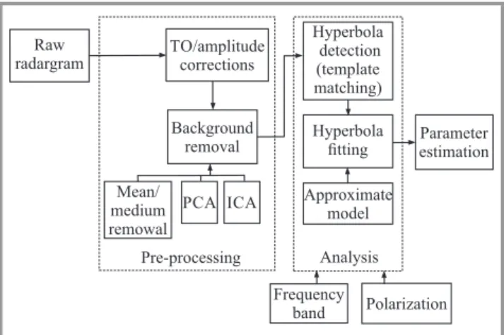
Fig. 1. The several stages of the processing link for the quanti-tative analysis of a radargram associated with buried targets. Thus, the data processing chain synthesized in Fig. 1 has been developed to particularly analyze theoretical and ex-perimental data sets. The processing is made of two main

stages associated with pre-processing and analysis algo-rithms to extract quantitative information from the hyper-bola signatures associated with detectable targets. The in-formation is relative to the evaluation of the target location, depth, size and dielectric nature. Attention has been paid to clutter removal in the case of a shallow target depth and a low permittivity contrast between the target and the soil, and on hyperbola detection in the presence of multi-ple targets and a heterogeneous soil. Parameters such as the frequency band and polarization have been considered as they can bring more detailed information from radargrams with additional processing.

2. The Measurements

The acquisition of radargrams was achieved using several GPR systems operating at frequencies ranging from 300 MHz to 1.5 GHz either in the time domain (GSSI SIR 3000, UtilityScan DF) or in the frequency domain (a SFCW GPR conceived in our laboratory). The SFCW (Step Frequency Continuous Wave) GPR is a laboratory system and cannot make at present fast measurements such as commercial sys-tems. The sampling distance step was around 5 mm using commercial GPRs, and defined to 40 mm using the labora-tory system. The two types of GPR systems were used to make comparisons, and results are presented in this paper at 900 MHz.

The SIR 3000 was equipped with one of the three antenna pairs operating at the central frequencies 500, 900 MHz and 1600 MHz, and the UtilityScan DF worked with a double frequency antenna system at 300 MHz and 800 MHz that is supposed to collect data at the same sampling distance because the switching device is rapid enough during walk-ing. Only the transverse magnetic (TM) polarization with respect to the pipe axes has been considered because these GPR systems only consider this polarization.

The SFCW GPR is made of a pair of shielded bowtie slot antennas (A4 sheet size designed on a single-sided FR4 substrate) has been used with a portable Anritsu MS 2026B Vector Network Analyzer (VNA) in the frequency band [0.05; 4 GHz] (1601 samples, intermediate frequency 500 Hz, 2 m coaxial N cables) [7]. A full two ports cal-ibration was made that allows to measure the fourSi j(f) coefficients.

Measurements in the frequency domain and in an Ultra-Wide Band (UWB) offer the advantages of selecting if needed a frequency band and shaping a Gaussian pulse as-sociated with this frequency band, and using easily the po-larization diversity. The complex transmission coefficient

˜

S21(f) measured at each scanning distance with a step of 40 mm is transformed in the time domain using an inverse Fourier transform to obtain a radargram. An apodization of each frequency curve has been made to smoothly extend the measured band from 4 to 9 GHz, and then perform the product with the spectrum of the excitation signal (the first derivative of the Gaussian function with duration 0.5 ns) used in Finite Difference Time Domain (FDTD)

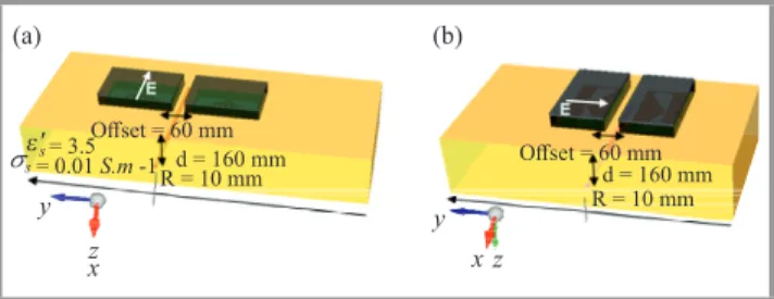
simula-tions. Two symmetric antenna configurations have been defined such as presented in Fig. 2 to consider two per-pendicular polarizations: the end-fire configuration (or TM mode) with both antennas aligned along their larger dimen-sion, and the broadside configuration or transverse electric mode (TE) with both antennas facing each other symmet-rically along their larger dimension. The laboratory made SFCW GPR has been easily modeled as all the antenna characteristics and geometry are known.

Fig. 2. The two polarization configurations of the SFCW GPR: (a) TM polarization (end-fire), and (b) TE polarization (broad-side).

The measurements have been performed in two different test sites:

• a large sandy box belonging to the public square Perichaux in Paris 15th district [8]. The sand was wet on the surface, and its permittivity has been esti-mated to a real permittivityεs′. A couple of canonical objects (pipe or blade) dielectric or conductive with lateral dimension less than 25 mm have been buried at a depth close to 160 mm. They have been sepa-rated by a distance around 750 mm;

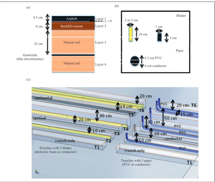
• an utility zone built under the urban test bed Sense-City in Marne-La-Vall´ee (France) [9]. This zone is under the 10 m wide traffic circle with lawn at the center. The underground contains two series of 5 trenches parallel to each other with size0.3×4m and separated by an offset of 40 cm (Fig. 3). Each target has been positioned in the middle of a trench at a depth ranging from 14.5 to 64.5 cm from the 4.4 cm thick asphalt surface. The two series of trenches include dielectric or conductive pipes (di-ameter 63 mm) and dielectric or conductive blades (thickness between 1 and 3 cm). The pipes have been filled with air or water. The trenches were filled with a soil of fine elements (without gravels) com-monly used in urban underground filling. The near sub-surface is made of four main layers correspond-ing to asphalt (layer 1), aggregate cement (layer 2), a natural soil (layer 3), and a quite wet natural soil (layer 4) located under a geotextile (a thin disconti-nuity). The real permittivities of the soil layers have been estimated as: asphalt (layer 1)ε′

1=4.5 (corre-sponding to a time propagation of 0.64 ns), aggregate cement (layer 2)ε′

2=7.7(1.4 ns), natural soilε3′=34 (8.5 ns).

Fig. 3. Structure of the sub-surface in Sense-City site: (a) the main multilayers of the soil, (b) geometries of the buried objects, (c) distribution of the buried pipes and strips.

3. Modeling

A 3D full-wave FDTD modeling using the commercial soft-ware EMPIRE has enabled to analyze EM phenomena as a function of parameters such as soil and pipe permittiv-ity, pipe depth, and antenna polarization and make com-parison with experimental results [8], [9]. The complete SFCW GPR made of a pair of shielded bowtie slot anten-nas (frequency band [0.46 ; 4] GHz) and designed on a FR4 substrate (real relative permittivityε′_{=4.4 and thickness}

e=1.6 mm) has been modeled in the presence of a semi-infinite soil [7]. Each antenna is enclosed in a shielded conductive rectangular box filled with a three-layered ab-sorbing foam with total dimensions 362×23×67.5 mm. The offset between antennas in simulations and experiments has been fixed to 60 mm, and the elevationhsabove the soil ishs=40 mm. The soil electrical parameters (εs′,σs) are assumed constant across the frequency range. The GPR

system is moved linearly on the soil surface with a step

∆y=40mm (see Fig. 2) to acquire a radargram. The ex-citation signal generally used in the simulations is the first derivative of the Gaussian function with a duration equal to 0.5 ns (99% of the total energy) and begins at 0.33 ns.

4. Pre-Processing

The pre-processing step aims to prepare radargrams be-fore analyzing the hyperbola signatures of sub-surface tar-gets to extract quantitative information. After time scaling and amplitude scaling (if needed), the main step consists of clutter removal to reduce the reflection component of the ground surface, direct waves between antennas, cou-pling between the antenna system, and a shallow target, as well as scattering induced by soil heterogeneities. The clutter often hides target signatures because its amplitude is far stronger and the arrival time is shorter. Several

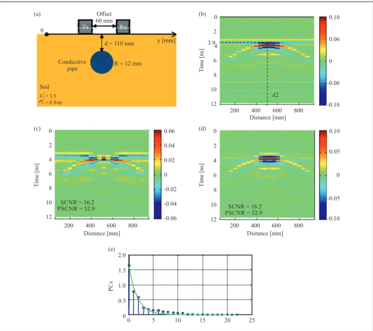
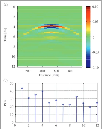
clut-Fig. 4. Pre-processing applied on a synthetic radargram issued from FDTD simulations: (a) geometry of the soil structure including a buried conductive pipe probed by a pair of shielded bowtie slot antennas (TM polarization), (b) raw radargram, (c) radargram processed by PCA, (d) radargram processed by PCA modified, (e) distribution of the PCs. (See color pictures online at www.nit.eu/publications/ journal-jtit)

ter reduction techniques were proposed in the literature and their development is an active research topic because the clutter is not uniform in a radargram, it is unsteady and it has different types [10].

The methods proposed appear initially suited to targets with small lateral dimension, overlapping hyperbola signa-tures, varying clutter along the scanning direction (a non-stationary signal), overlapped target and clutter signals in time and frequency [11]. The semi-automatic methods tested and compared are the mean or median subtrac-tion [12], the Principal Component Analysis (PCA) that has been modified and the Independent Component Anal-ysis (ICA) [13], [14]. Basically, PCA relies on the second order statistics to perform the correlation analysis, whereas ICA requires higher order statistics (4th moment). Both

methods have the advantage of requiring limited prior in-formation on the data set.

4.1. PCA

The objective of PCA is to express the original data set in another domain by means of any appropriate linear transfor-mation. PCA is a subspace projection method that is based on either on a Singular Value Decomposition (SVD) or an Eigenvalue Decomposition (EIG) to select relevant compo-nents in different subspace projections [13]. Each eigen-value is related to a certain eigenvector (principal com-ponent), and the eigenvalues are ordered in the descending order. The main problem of this algorithm is how to choose the principal components where information is contained.

Every eigenvalue represents a specific amount of variance in measured data, and the objective is to obtain a new set of uncorrelated data.

From the initial data matrix X(M×N) (with M ampli-tude signals A-scans and N time samples; M <N) the firstk1components associated with the clutter and the last

N−(k2+1)components associated with noise are generally removed thus giving a new data set:

X0= k2

∑

k1+1

uisivTi , (1)

whereui andvi are eigenvectors.

However, difficulties can be met when the clutter does not have the highest energy within the radargram in the case of a target that induces a strong Radar Cross Section (RCS) such as a conductive or a water filled target, or a high contrasted dielectric target with the surrounding soil [15]. Moreover, it appears difficult to select the index rank de-fined by k1 and k2 when there are multiple targets and reflections. Thus, we have proposed to modify PCA and apply the algorithm on a radargram with a reduced time scale (investigation depth) and a splitting of the scanning scale associated with a selected hyperbola signature into 3 parts. This splitting is based on an energy criterion that compares energy in the apex area and energy in the arms. This splitting allows to analyze separately the area close to the apex and relative to the two arms as they show dis-tinct amplitude value and interaction with the clutter. It particularly concerns target response with high energy that is comparable to the clutter energy.

An illustration of the application of PCA and PCA mod-ified is presented in the case of a conductive pipe with radius R=12 mm (see Fig. 4a), buried at a depth d of 110 mm (that is, 3₄ of the wavelengthλsoil at 1 GHz) in a soil with real permittivityε′=3.5( d

λsoil ≈1 at 1 GHz), that has been probed by the pair of bowtie slot antennas used in the SFCW GPR (TM polarization). The data set have been obtained from FDTD simulations (see Fig. 4b) and, in this case, there is overlapping between clutter and hyperbola response. The arrival times of the clutter and the target are 3.4 and 3.9 ns, respectively. The PCs selected represents 90% of the energy, the first one is removed as it represents the clutter component (see Fig. 4e). The pro-cessing by conventional PCA depicts visually bad perfor-mance in reducing the coupling between antennas as part of the horizontal component of antenna coupling remains (see Fig. 4c). PCA modified preserves the target hyperbola shape (see Fig. 4d) but it does not eliminate completely the clutter over the apex, and a clutter remains in the time interval 3. . .4 ns.

4.2. ICA

ICA has been recently proposed as an alternative to eigen-vector decomposition in radar images as it has proved it-self to be a very promising tool to better interpret non-Gaussian heterogeneous clutter. ICA that is based on higher

order statistical moments, can recover statistical indepen-dent sources and the mixing mechanism without having any physical background of the latter [14], [15]. The ICA model associated with a data matrixX that is assumed ran-dom is generated from a source matrix S through a linear process:

X=SA, (2)

where X is the matrix used in the PCA algorithm, S= (s1,s2, . . . ,sN2)is theM×N2source matrix (N2≤N), and

A is theN2×Nmixing matrix.

ICA assumes that the components of the source matrix are statistically independent with respect to each other, that makes ICA more efficient in the separation process. Before processing with the calculations, X is transposed (XT =ATST) and then ICA uses centering, whitening, and dimensionality reduction algorithms as pre-processing steps to simplify and reduce the complexity of the problem. The FastICA algorithm (fixed-point algorithm first proposed by Hyv¨arinen and Oja [15]) available in a Matlab package leads to the determination of two sub-solutions: 1) the esti-mation of the mixing matrixA, and 2) the estimation of the source signalsS. To measure the non-Gaussianity (the in-dependence) of the sources a non-linear and non-quadratic function, also called a contrast function, is used that helps to optimize the performance of the ICA algorithm. In this work, negentropy has been used to measure the non-normality or the degree of unstructuredness of a

ran-Fig. 5. Pre-processing applied on the synthetic radargram of Fig. 4a using ICA: (a) radargram processed by ICA, (b) Kurtosis criterion applied on ICs.

dom vector. Negentropy is non-negative and has a high value for non-Gaussian variables. In practice, negentropy is difficult to calculate and must be approximated, a solu-tion proposed by Hyv¨arinen [15]. An iterasolu-tion based on the fast-fixed-point technique that uses random vectors as starting values, allows to estimate step by step the sev-eral independent components (ICs). Afterwards, the main difficulty relies on the selection of ICs which contain in-formation. The Kurtosis criterion applied to the ICs has served to define a threshold beyond which the ICs selected contain information.

As an illustration, the previous synthetic radargram associ-ated with a conductive pipe buried at 110 mm depth has been analyzed by the ICA algorithm. The results in Fig. 5a show that the clutter is better reduced by ICA than by PCA modified, as there is no artifact above the apex, however a weak horizontal clutter remains visible. The Kurtosis criterion applied on ICs are plotted in Fig. 5b.

4.3. Comparison Criteria between Processing Algorithms

The visual comparison of the reconstructed images with re-duced clutter provides a first qualitative assessment of the algorithms tested. Attention has to be paid to spatial co-herency along the scanning direction in such a way that the visibility of a hyperbola must be strengthened as compared to that of the clutter. Thus, a few tools have been used to quantitatively compare the performance of the clutter reduction algorithms.

Signal to Clutter and Noise Ratio (SCNR)

The ratio is defined as the average energy of the recon-structed clutter-reduced image (represented by a matrixF

of real values fi,j withi=1, . . . ,M and j=1, . . . ,N) with the average energy contained in the “noise” image (named

Gwith elements gi,j with i=1, . . . ,M and j=1, . . . ,N), that is obtained by subtracting the raw image from the pro-cessed image such as [17]:

SCMRdB=10 log Ptarget Pclutter+noise = 10 log ∑ i=1,Nj=∑1,M |fi,j|2 ∑ i=1,Nj=∑1,M |gi,j−fi,j| 2. (3)

In practice, we don’t have the opportunity to acquire an im-age without clutter and noise, that limits the interpretation of the SCNR.

Peak Signal to Noise and Clutter Ratio (PSCNR) Another parameter is the PSCNR that uses presently the peak signal instead of its average energy such as [18]:

PSCNRdB=10 log NMmax(|f|)2 ∑ i=1,Nj=∑1,M |gi,j−fi,j| 2. (4)

Again, this ratio has some limits.

Receiver Operating Characteristics (ROC) curves ROC curves appear more appropriate to compare quanti-tatively clutter reduction algorithms. The ROC curve is simply a graph of detection versus false alarm probabilities parameterized by a threshold S [19]. From a ROC curve (1×1 square region), fundamental information extracted from metrics (in general area-under-roc-curve AUC) is de-rived. A ROC curve is calculated by comparing pixel to pixel two binary images, a reference image containing only the desired information and the image processed by an al-gorithm using a varying thresholdSin the amplitude range of the raw image. The reference image defined corresponds to a skeleton of the hyperbola response including the first positive and negative amplitudes. The threshold applied on the raw image serves to compute a binary image to make a comparison with the reference image.

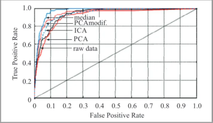
As an illustration, these 3 parameters have been evaluated for the radargrams of Figs. 4c-d (PCA), and also Fig. 5a (ICA). The largest SCNR and PSCNR values belong to the median subtraction technique (14 and 72.9 respectively), and afterwards the better performances are attributed to PCA modified and ICA. The ROC curves visualized in Fig. 6 show that the curve associated with PCA is slightly below the one issued from the raw data. The curve as-sociated with PCA modified appears higher than the one belonging to ICA.

Fig. 6. ROC curves associated with the different pre-processing algorithms (median subtraction, PCA, ICA) applied on the raw radargram of Fig. 4a.

As a conclusion, the median subtraction technique appears a robust method for clutter reduction but it has its limits in the case of the overlapping of clutter and hyperbola re-sponse. As a conclusion, the median subtraction technique appears a robust method for clutter reduction that has how-ever its limits, in the case of overlapping between clutter and hyperbola response. The PCA algorithm shows bet-ter performance in the case of the relative pipe diamebet-ter

d

λsoil ≤0.7 and when there exists partial overlapping be-tween clutter and hyperbola. When the hyperbola response has a high amplitude, PCA modified improves the removing of the clutter The ICA algorithm shows better performance in the case _λd

5. Hyperbola Detection and Fitting

In practice, the difficulties encountered in hyperbola detec-tion in a radargram rely on the heterogeneity of the back-ground and a weak contrast between the hyperbola and the background. Thus, we have proposed a semi-automatic de-tection algorithm based on template matching that doesn’t require a training period [20]. It is applied after a pre-processing stage and is made of a series of steps:

• A template containing a typical hyperbola signature is built, that is issued from synthetic or experimental data. The template does not need to be fully similar to the responses to be detected. When the hyperbolas in the radargram cannot be detected by a single pat-tern, several patterns can be used in sequence. Each defined template includes a small portion of a hyper-bola signature near the apex. It has to be scaled in time, distance and amplitude to the radargram that has to be analyzed.

• An amplitude distance map is calculated by trans-lating on the radargram the predefined template at every possible positions. A mean amplitude distance is evaluated according to the L1norm.

Assuming an observed image G with elements gi,j org(i,j) and size M×N, and a template image T

with elementsti,j ort(i,j), both images with scaled amplitudes, we define the L1 norm distance mapE

betweeng andt by the following relation [18]:

E(m,n) = M

∑

∑

The summation is evaluated at all pixels (i, j) of the template t that is translated to all possible po-sitions (m,n) along the observed image g. The po-sition (m,n) at which the smallest valueE(m,n) is obtained corresponds to the best match between the templatet and the corresponding sub-image ing.

• A threshold value increased progressively by the user allows to select a number of minima on the distance map that corresponds to a high level of similarly with the template.

• At the selected positions, the hyperbola points close to the apex that correspond to a maximum or a mini-mum amplitude have to be extracted. Because higher order reflections in a hyperbola pattern may produce a stronger amplitude as compared to the amplitude of the first reflection, an user interaction is necessary (semi-automatic) to select a hyperbola curve either on the upper or on the lower half zone of the central template position. Starting from the vertical symme-try axis of the template, close points belonging to the hyperbola curve on the left and on the right legs (usually 3 or 4 points) are extracted step-by-step. Be-cause the number of curve points extracted is limited,

a polynomial fitting of the second order was made to refine the estimate of the abscissay0at the apex.

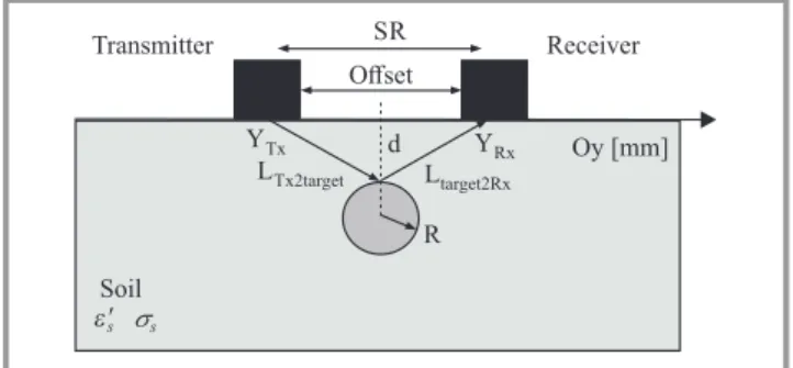
• The estimation of the several parameters describing the hyperbola curve such asd,R,V, the target depth and radius and the celerity in the soil, respectively (see Fig. 7) is obtained using a hyperbola fitting of the curve points to the classical analytical relation according to the LS criterion. Parameters SR andy0, representing respectively the center-to-center distance between antennas and the horizontal coordinate of the object, are a priori known. The position of the radar referenced at the center of the system is located using coordinateyk.

Fig. 7. Cross-view of a pipe buried in a soil and parameters associated with the ray-path theory.

The equations associated with the travel-time write as fol-lows [21]: ( yT=yk−SR₂ yR=yk+SR₂ , (6)      TT x2target= h (y0−yT)2+ (d+R)2 i1₂ −R Ttarget2Rx= h (y0−yR)2+ (d+R)2 i1₂ −R , (7)

where TT x2target and Ttarget2Rx represents the ray paths be-tween the transmitter or the receiver to the buried object. The velocity vof the medium depends on the real relative permittivityε′ s such as: v=pc ε′ s ; (εs′′≪εs′). (8) The generalized hyperbola equation (yk,tk) including the antenna offset is expressed by:

tk=

TT x2target+Ttarget2Rx

v . (9)

Thus, (y0,t0) represents the position in coordinate and time of the maximum of the hyperbola. It must be un-derlined that the hyperbola depends on five parameters (SR,y0,d,R,v). In general, the pipe radius cannot be prop-erly estimated, as it appears smaller than the radiating aper-ture of one antenna (on the order of the first Fresnel zone in the soil). The minimum of the sum of squares of the

distances between theoretical yk,theo and measuredyk,meas data has been solved using the Gauss-Newton method as follows: F= K

∑

Some constraints relative to the parameter ranges have been added in the algorithm to better drive the solution. The Hessian matrix in 2D and particularly its eigenvalues can be used to characterize the uncertainties on the esti-mated parameters(d,v).

5.1. Application to Experimental Data

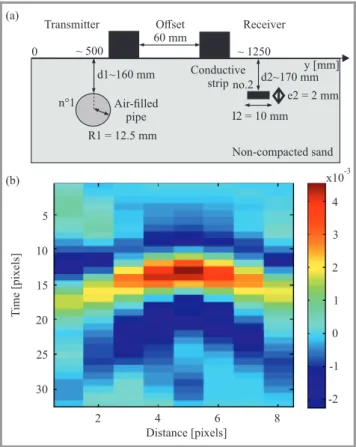
In the sandy box of the public square Perichaux, Paris 15th, the dielectric permittivity of the soil at this moment was estimated to 3.5 from common mid-point (CMP) measure-ments. Two targets, a 25 mm diameter dielectric pipe filled with air and a thin horizontal 10 mm width (2 mm thick) conductive strip were buried at the depths estimated to 160 and 170 mm respectively such as presented in Fig. 8a. Both objects are separated by a 750 mm distance. The scanning by the SFCW GPR has been performed in both end-fire and broadside polarizations (see Figs. 2a-b). A synthetic template was computed from 3D FDTD sim-ulations (software Empire) considering the detailed bowtie

Fig. 8. Geometry of the sandy box with two buried objects, an air-filled pipe and a horizontal conductive strip (a), synthetic template issued from FDTD simulations involving a pair of bowtie slot antennas (end-fire configuration) moved on a soil (ε′

s=3.5,

σs=0.01Sm−1, hs=10 mm) with a buried conductive pipe

(R=12.5mm) (b).

slot antenna geometry (Section 3) and 32 mm radius con-ductive pipe buried in a soil with a real relative permittivity ε′_{=3.5 (σ=10}−2_Sm−1_{). The end-fire configuration has} been considered. In this template visualized in Fig. 8b, it was wise to define a compact hyperbola signature with reduced multiple reflections to further detect different hy-perbolas in a radargram in both polarizations. The template was scaled in time and amplitude to match the experimen-tal time step∆t=5.56·10−2ns (step distance 40 mm used in the experiments), and the amplitude range of the experi-mental radargrams. Signed amplitudes have been used here to not deteriorate the image quality.

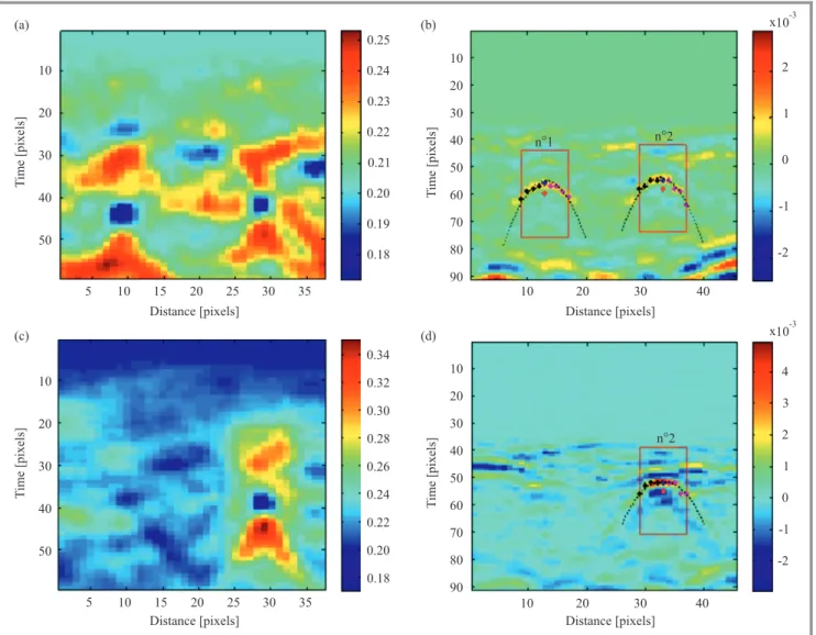
The template matching algorithm proposed has been per-formed on experimental radargrams considering the two or-thogonal polarizations after application of the median sub-traction technique. Results are presented for the geometry relative to Fig. 8a, and the time range has been defined to 5 ns. That leads to the L1 norm distance maps (also abso-lute distance maps) visualized in Figs. 9a and 9c. The posi-tion (m,n) at which the smallest valueE(m,n)is obtained corresponds to the best match between the template t and the corresponding sub-image ing. A threshold value allows to select a limited number of local minima corresponding to distances less than the threshold where the template is well matched with enough amplitude (visualized by “+” signs on the radargrams). The maximum threshold values leading to the detection of the most significant hyperbolas are 0.162 and 0.195 in the broadside and end-fire configu-rations, respectively (see Figs. 9b and 9d). Higher values give additional detections (false alarms) that don’t corre-spond to buried objects but to background heterogeneities. In the end-fire polarization, the distance map cannot permit to detect the air-filled pipe.

The results of the parameter evaluation from the least-square (LS) fitting of each hyperbola detected are col-lected in Tables 1 and 2. In general, the positions y0 of the objects appear correctly evaluated. Concerning the real permittivity value of the soil, the broadside configuration gives higher estimates as compared to the end-fire configu-ration, and consequently the target depths appear more im-portant.

Table 1

Parameter estimation in the broadside configuration for the experimental B-scan of Fig. 9b (max. is associated

with the detection of the positive amplitude) Object d R ε′ T0 y0 fval [mm] [mm] [ns] [mm] Pipe no. 1 200 60 3.6 3.08 458.9 2.68·10−2 (max) Pipe no. 1 ∼160 12.5 3.5–4 ∼500 (true values) Strip no. 2 200 60 3.47 2.99 1232 2.23·10−2 (max.) Strip no. 2 ∼170 5 3.5–4 ∼1200 (true values)

Fig. 9. Analysis of experimental radargrams (in pixels, time range 5 ns) associated with an air-filled pipe and a horizontal conductive strip using the template matching algorithm: (a, b) in the broadside and (c, d) end-fire configurations; (a, c) time-distance maps, (b, d) positions of the image template in the original B-scans and hyperbola fitting.

Table 2

Parameter estimation in the end-fire configuration for the experimental B-scan of Fig. 9d Object d R ε′ T0 y0 fval [mm] [mm] [ns] [mm] Strip no. 2 165.6 25.5 2.65 2.82 1250 1.85·10−2 (max.)

From Table 3 that collects eigenvalues of the Hessian ma-trix at the estimates of the depth and the velocity (d,v), we remark that the depths of the pipe and the strip have been both estimated to 200 mm, and more important than those a priori known (see Fig. 8a). In the case of a soil having weak permittivity variations, an additional step would be to find an optimum permittivity value issued from the sev-eral estimates. We remark that the objective functionfval associated with the LS fitting is presently higher for exper-imental data than for synthetic data of the order of10−2, because the image quality appears lower.

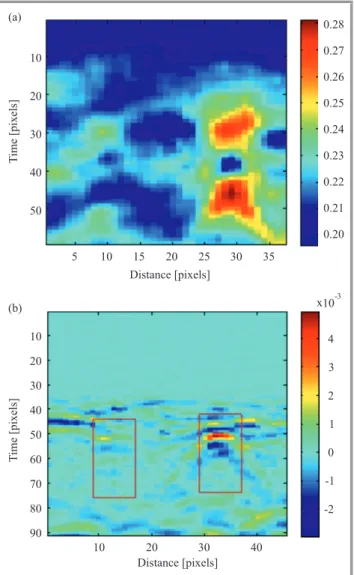
To detect the air-filled pipe in Fig. 9d, joint information from radargrams issued from the parallel and end-fire con-figurations (polarization diversity) could be used. Thus, the mean distance map was calculated from the individ-ual distance maps in the broadside and end-fire configura-tions (see Figs. 9a and 9c) leading to the result visualized

Table 3

Eigenvalues of the Hessian matrix at the estimates of the depthd and velocityvfrom hyperbola fitting

in both polarizations

Configuration Eigenvalues for(d;v) Parallel

Pipe no. 1 (4.1·10−5; 2.1·10−2) Strip no. 2 (4.2·10−5; 1.9·10−2)

End-fire

in Fig. 10a. A weak threshold (0.18) situated between the previous ones (0.162 and 0.195) associated with both po-larizations (see Fig. 10b), has allowed here to detect both hyperbolas without false alarms in the end-fire configura-tion, that was not possible when this polarization was only considered. Further insight into the solutions of the param-eters estimated in the fitting has been gained by calculating the Hessian matrixHat the stationary point to evaluate its nature using its eigenvalues.

Fig. 10. Mean distance map in the parallel and end-fire configu-rations associated with an air-filled pipe and a horizontal conduc-tive strip (Fig. 8a) (a) and positions of the image template in the experimental B-scan in the end-fire configuration (b).

The rate of convergence and sensitivity to round-off errors is given by the condition number of matrix H, that is the ratio of its largest to its smallest eigenvalues. In the present examples, fixing the pipe radius that cannot be evaluated properly has led to a decrease of the condition number. The eigenvalues associated with the several fittings in both polarizations are collected in Table 3. In general, the condi-tion number is high, that means that correlacondi-tion may exist between the two parameters and thus the convergence of the estimation algorithm appears slow.

6. Polarization Diversity

As a target can depolarize the incident field, thus giving a scattering response depending and the orientation of the antennas relative to the target, it is worth to exploit the polarization to characterize the target, and its orientation, particularly in the case of a long target such as a cylinder.

6.1. Analytical Modeling

The influence of the dielectric characteristics of a canonical target such as a cylinder (index d) illuminated by a elec-tromagnetic (EM) polarized plane wave is described by the scattering theory [16], [23]. The backscattered fields de-pend strongly on the orientation of the cylinder relative to the antennas, its dielectric properties, and the radius of the cylinder compared to the wavelengthλ0in the surrounding medium (index 0). The medium is usually air, but can be a dielectric material such as considered here. The scatter-ing properties of a long cylinder has been described by the Bessel and Hankel functions. The scattering width (SW) is the equivalent area proportional to the apparent size of the target (in the far-field zone) that scatters the field relative to the incident power in each directionφ. Four expressions associated with SW consider both TE and TM polariza-tions and the case of a dielectric or a conductive cylinder as follows [23]: TE polarization Conductive cylinder: SW =2λ0 π +∞

∑

∑

∑

∑

Fig. 11. Influence of the pipe radius and the real permittivity on the scattering width (SW) as a function of the frequency in the case of (a, b) a conductive and (c, d) a dielectric air-filled cylinder (ε′_{=1in “c” andε}′_{=9in “d”).}

where β0 and βd are the wavenumbers, associated with the surrounding medium and the dielectric cylinder; they can be complex. Jn(.) is the Bessel function of the first kind of ordern,J_n′(.)is its derivative,Hn(2)(.)is the Hankel function of the second kind of ordern, andHn(2)′(.)is its de-rivative.

The simplified modeling of the GPR system considers that the antennas, linearly polarized, are closely spaced. This results to a backscattering angle corresponding toφ=180◦. Before analyzing theoretical and experimental B-scans, we have studied the scattered responses SW in a very large fre-quency band [0.2 ; 2] GHz considering several pipe radii and two dielectric contrasts between the pipe and the sur-rounding medium. The results collected in Figs. 11a-b, in the case of a conductive cylinder with a radius in the range5. . .40mm, highlight that the TM polarization (elec-tric field parallel to pipe axis) generally leads to a higher backscattering response whatever the value of the real per-mittivity value (ε₀′ orε₀′′=0) of the surrounding medium. We remark that the TE component oscillates under the TM component for a radius higher than 5 mm. In general, the

scattering width increases with the pipe radius and when the radius becomes large as compared to the wavelength of the medium; at 2 GHz,λ0=75mm forε′

0=4, andλ0=50mm for ε₀′=9. Consequently, the TM polarization is preferred to detect a conductive pipe independently of its radius and the wavelength of the surrounding medium. Figure 11c-d associated with a dielectric cylinder show that the TE polar-ization gives a higher SW when the radius value is inferior to the wavelength and when the permittivity of the pipe (here filled with air) is less than the medium permittivity (ε′

0=4). When the pipe is more dielectric (ε0′ =9) than the medium, we remark that the TM polarization is in gen-eral higher than the TE polarization. We also observe that for a radius greater than 10 mm, TE and TM components oscillate and they can meet each other.

6.2. In-situ Measurements

The measurement results presented have been made in the test bed Sense-City (see Fig. 3). To facilitate the subsequent interpretation of vertical profiles with buried pipes, refer-ence measurements were performed apart from the areas

with buried objects to obtain the dielectric characteristics of the multilayered soil. Using the commercial GPR GSSI SIR 3000, a scanning has been acquired to identify the several layers of the sub-surface. Consistently with the di-rect observations during excavation, the raw radargram at 900 MHz (without time zero correction and clutter removal) shown in Fig. 12 shows a soil made of four layers corre-sponding to asphalt (layer 1), aggregate cement (layer 2),

Fig. 12. Experimental radargrams (B-scans) of the subsurface without buried objects measured by the SIR 3000 system (linear gain and low and high pass filters applied) at 900 MHz in the TM polarization.

a natural soil (layer 3), and a wetter natural soil (layer 4) located under the geotextile (a thin discontinuity). A sub-layer of sub-layer 3 (sub-layer 3b) of natural soil under the aggregate cement appears visible in this zone of the site and it is at-tributed to a compacted layer of natural soil. This layer will not be observed in the zone with the trenches because the soil has been excavated. From the radargram at high res-olution, we have estimated the real permittivitiesε′ _since we have an a priori knowledge of the thicknessh of each layer from the construction phase. According to Fig. 3a, the real permittivity estimations of the soil layers are the following: asphalt (layer 1)ε′

1=4.5 (0.64 ns), aggregate cement (layer 2) ε′

2=7.7 (1.4 ns), natural soil (mean of layers 3b and 3)ε′

3=34 (8.5 ns). Based on these results,

a mean real permittivity of 12.7 is derived (decomposition in volumetric fractions).

Measurements have been made manually using the SFCW georadar system on the pipe zone of the test site whose cross section is presented in Fig. 13. The radargrams are presented in the time domain in both TE and TM polariza-tions (see Figs. 14a-b) considering a pulse with a peak fre-quency at 900 MHz. Neither low pass, nor high pass filters and nor time zero correction were applied here. The pipe in T5 was filled with air. A linear time gain [–10 ; 20] dB was applied to the radargram of Fig. 14a in the TE polariza-tion (broadside). We remark in this figure that the air-filled pipe at depth 30 cm in T4 shows a detectable hyperbola signature (contrary to the SIR 3000 results). The signature of trench T1 appears weakly detectable, certainly because the distance step (4 cm) has not been defined here small enough (this will be improved in the future). In the TM polarization (end-fire), such as visualized in Fig. 14b, the measurements were made in two sequences that explains the vertical discontinuity in the radargram. In general, we re-mark that all the hyperbolas appear strongly attenuated that is consistent with the synthetic radargram obtained from FDTD simulations [22].

7. Conclusion

In this work, signal and image processing techniques have been collected with the aim of extracting quantita-tive information from experimental radargrams containing hyperbola signatures from pipes and strips with lateral di-mension less than around ten centimeters. The difficulties met in the analysis of GPR radargrams is the detection of a hyperbola pattern in a noisy background, in a weak image quality, with overlapping between signatures of the clutter and one or multiple targets (particularly buried in a shallow depth), and also the detection of a target with a small lateral dimension and a weak contrast with a per-turbed surrounding medium. The main objective was to propose a data processing chain easily implementable to analyze by steps radargrams made of hyperbola signatures associated with relatively small pipes (less than 100 mm). Thus, a semi-automatic data processing has been proposed that is supposed to be adaptable to hyperbola signatures

Fig. 14. Experimental radargrams measured by the SFCW GPR system in the: (a) TE (broadside), and (b) TM (end-fire) polar-izations.

countered in a generally noisy and heterogeneous environ-ment showing different dielectric contrasts with the tar-gets. It has been observed that to remove the clutter, deep and shallow targets must be distinguished. In the case of a shallow target, which significantly influences the clut-ter and the inclut-terface reflection, the PCA algorithm appears in general more efficient than ICA. In the case of a deep target, ICA appears to be more efficient than PCA. The template matching algorithm has been adapted to the hy-perbola detection by means of the definition of a adequate template that represents a hyperbola shape close to the apex. The template has been generated from FDTD simulations. The algorithm has been validated on experimental radar-grams, and has been extended to take advantage of data sets that consider the polarization diversity. This addi-tional parameter improves the algorithm robustness. Fu-ture researches aim at applying the template matching al-gorithm on radargrams with different target shapes (pipe and cracks) and dielectric contrasts with the surrounding soil. Improvement of the data processing chain could be made by adding complementary algorithms such as

space-frequency time-reversal matrices [24], wavelet transform, or hyperbola detection that accounts for hyperbola miss-hapedness [25].

Acknowledgment

The author would like to thank colleagues belonging to several laboratories of IFSTTAR: Vincent Baltazart, Xavier Derobert, Elias Tebchrany, Bereng`ere Lebental and Erick Merliot for their contribution in the different scientific parts to these researches during the past three years.

The author greatly acknowledges the COST Action TU1208 for proposing members to publish their recent research in applied electromagnetics.

References

[1] Z. Liu and Y. Kleiner, “State of the art review of inspection tech-nologies for condition assessment of water pipes”, Measurement, vol. 46, no. 1, pp. 1–15, 2013.

[2] H. O. Henriques, M. Z. Fortes, L. Hudson, N. S. V. Silva, and F. O. Teixeira, “Use of radar illegal connections prospecting in buried or embedded cables”,Measurement, vol. 47, pp. 221–227, 2014.

[3] CI/ASCE38-02, American Society of Civil Engineers, Standard guideline for the collection and depiction of existing subsurface util-ity data, 2002.

[4] ASTM Designation D 6432-11, Standard Guide for Using the Sur-face Ground Penetrating Radar Method for SubsurSur-face Investigation, 2011.

[5] Italian Standard CEI-883, Regulations for performing preliminary surveys with ground-probing radar for before laying underground utilities and infrastructures, 2004.

[6] Proceedings of the First General Meeting of COST Action TU1208, L. Pajewski, and A. Benedetto, Eds. Rome, Italy, July 2013, Aracne, Rome, Italy, July 2013 [Online]. Available: http://www.cost.eu/ domains actions/tud/Actions/TU1208

[7] F. Sagnard, “Design of a compact ultra-wide band bow-tie slot an-tenna system for the evaluation of structural changes in civil en-gineering works”, Progress in Electromag. Res., PIER B, vol. 58, pp. 181–191, 2014.

[8] F. Sagnard and E. Tebchrany, “Using polarization diversity in the detection of small discontinuities by an ultra-wide band ground pen-etrating radar”,Measurement, vol. 61, pp. 129–141, 2015. [9] F. Sagnard, C. Norgeot, X. Derobert, V. Baltazart, E. Merliot,

F. Derkx, and B. Lebental, “Utility detection and positioning on the urban site Sense-City using Ground Penetrating Radar Systems”, Measurement, vol. 88, pp. 318–330, 2016.

[10] R. Solimene, A. Cuccaro, A. Dell’Aversano, I. Catapano, and F. Sol-dovieri, “Ground clutter removal in GPR surveys”,IEEE J. of Se-lec. Topics in Appl. Earth Observ. and Remote Sensing, vol. 7, no. 3, pp. 792–798, 2014.

[11] E. Tebchrany, F. Sagnard, V. Baltazart, and J. P. Tarel, “Data pro-cessing of ground-penetrating radar signals for the detection of discontinuities using polarization diversity”, European Geoscience Union General Assembly 2014, Vienna, Austria, 27 Apr. – 2 May 2014.

[12] G. T. Tesfamariam, D. Mali, and A. M. Zoubir, “Clutter reduction techniques for GPR based buried landmine detection”, inProc. Int. Conf. on Signal Process., Commun., Comput. and Netw. Technol. ICSCCN 2011, Thuckalay, India, 2011, pp. 182–186.

[13] I. T. Jolliffe,Principal Component Analysis, 2nd ed. Springer, 2002. [14] A. Hyv¨arinen, “Independent component analysis: recent advance”, Philos Trans. A Math. Phys. Eng. Sci., vol. 371, no. 1984, 2013 (doi: 10.1098/rsta.2011.0534).

[15] A. Hyv¨arinen and E. Oja, “Independent component analysis: algo-rithms and applications”,Neural Netw., vol. 13, no. 4, pp. 411–430, 2000.

[16] S. J. Radzevicius and J. J. Daniels, “Ground penetrating radar polarization and scattering from cylinders”, J. Applied Geophys., vol. 45, pp. 111–125, 2000.

[17] H. M. Jol,Ground Penetrating Radar Theory and Applications. El-sevier, 2008.

[18] P. K. Verma, A. N. Gaikwad, D. Singh, and M. Nigam, “Analysis of clutter reduction techniques for through wall imaging in UWB range”,Progress in Electromag. Res. B, vol. 17, pp. 29–48, 2009. [19] T. Fawcett, “An introduction to ROC analysis”,Pattern Recogn. Lett.,

vol. 27, no. 8, pp. 861–874, 2006.

[20] F. Sagnard and J. P. Tarel “Template-matching based detection of hyperbolas in ground-penetrating radargrams for buried utilities”, J. of Geophys. and Engin., vol. 13, no. 4, pp. 491–504, 2016. [21] S. Shihab and W. Al-Nuamy, “Radius estimation for cylindrical

objects detected by ground penetrating radar”,Subsurface Sensing Technol. and Appl., vol. 6, no. 2, pp. 151–166, 2005.

[22] D. Vernon,Machine Vision-Automated Visual Inspection and Robot Vision. Prentice Hall, 1991.

[23] C. A. Balanis,Advanced Engineering Electromagnetic. Wiley, 1989. [24] M. E. Yavuz, A. E. Fouda, and F. L. Teixeira, “GPR signal enhance-ment using sliding-window space-frequency matrices”,Progress in Electromag. Res., vol. 145, pp. 1–10, 2014.

[25] L. Mertens, R. Persico, L. Matera, and S. Lambot, “Automated de-tection of reflection hyperbolas in complex GPR images with no a priori knowledge on the medium”,IEEE Trans. Geosci. and Re-mote Sens., vol. 54, no. 1, pp. 580–596, 2016.

Florence Sagnardreceived the B.Sc. and the D.E.A. degree in Electronics from Universit´e Pierre et Marie Curie, France, in 1990 and the Ph.D. degree from Universit´e d’Orsay, Fran-ce, in 1996. In 2005, she was qualified to conduct researches (HDR) from Universit´e de Marne-La-Vall´ee, France. From 1997 to 2006, she was Assis-tant Professor at Université de Marne-La-Vall´ee and worked in the laboratory ESYCOM on the microwave character-ization of materials. From 2002 to 2006 she worked as an invited researcher at INSA (Institut National des Sci-ences Appliqu´ees), Rennes in UWB antennas, and trans-mission links. In 2007–2009, she joined CEREMA (Centre d’Etudes et d’expertise sur les Risques, l’Environnement, la Mobilité et l’Am´enagement), Rouen, and since 2010 she is with IFSTTAR Marne-La-Vallée to develop SFCW GPR systems. Her research interests include data and image pro-cessing, FDTD simulations, UWB antennas, soil character-ization, and civil engineering.

E-mail: [email protected] Université Lille Nord de France IFSTTAR

20 rue Elis´ee Reclus