Methods for Improving Challenging DNA Profiles and Molecular Preservation of Soft Tissue Samples

(1)

Methods for Improving Challenging DNA

Profiles and Molecular Preservation of Soft

Tissue Samples

by

Lais Vicente Baptista

A thesis submitted in partial fulfilment for the requirements for the degree of Doctor of Philosophy at the University of Central Lancashire

(2)

ii

STUDENT DECLARATION FORM

I declare that while registered as a candidate for the research degree, I have not been a registered candidate or enrolled student for another award of the University or other academic or professional institution.

I declare that no material contained in the thesis has been used in any other submission for an academic award and is solely my own work.

No proof-reading service was used in the compilation of this thesis.

Lais Vicente Baptista

Type of Award: Doctor of Philosophy

(3)

iii Essa cova em que estás,

com palmos medida, é a cota menor que tiraste em vida. — É de bom tamanho, nem largo nem fundo, é a parte que te cabe neste latifúndio.

— Não é cova grande. é cova medida,

é a terra que querias ver dividida.

— É uma cova grande para teu pouco defunto, mas estarás mais ancho que estavas no mundo. — É uma cova grande para teu defunto parco, porém mais que no mundo te sentirás largo.

— É uma cova grande para tua carne pouca, mas a terra dada não se abre a boca. Morte e Vida Severina, João Cabral de Melo Neto

The grave you’re in Is measured by hand, The best bargain you got In all the land.

– You fit it well, Not too long or deep, The part of the latifundio Which you will keep. – The grave’s not too big, Nor is it too wide,

It’s the land you wanted To see them divide. – It’s a big grave For a body so spare, But you’ll be more at ease Than you ever were. – You’re a skinny corpse For such a big tomb, But at least down there You’ll have plenty of room. – The grave is big

For your skin and bone, But when land is given, You can hardly moan. Death and Life of Severino, (John Milton translation)

(4)

iv

To my grandfather, my example of loving knowledge, and who always showed me the joy of learning and curiosity.

(5)

v

ABSTRACT

Degradation of DNA can lead to either poor quality, imbalanced, or even no profiles. Therefore, appropriate collection and storage methods are critical to minimize its impact. If the DNA is degraded prior to sample collection, then the degradation process can only be arrested and other methods have to be employed to try to improve the quality of the DNA profile. The major aims of this thesis were to assess alternative methods for molecular preservation of muscle tissue samples and to obtain better DNA profiles from degraded samples. Assessment of DNA degradation was undertaken using an in-house PCR assay which amplifies four amplicons from 70 bp to 384 bp. DNA degradation was evaluated in whole pig carcasses exposed to hot and humid environmental conditions. A full DNA profile could be generated for 24 hours, but some full profiles were obtained from samples taken as late as 72 hours. It was determined that when collecting tissue samples from partially decomposed bodies, those should be preferentially from the surface of the body in touch with the ground, as the results show that DNA persistence is improved.

In order to compare field and laboratory degradation patterns, muscle tissue samples were incubated in the laboratory at 25 °C and 37 °C. The persistence of DNA was increased when compared to field, most likely due to the lack of insect activity and of variations in temperature and humidity. Partially degraded muscle samples were preserved with 96% ethanol, cell lysis solution, or cell lysis solution with 1% sodium azide, which had been stored at room temperature for seven years. Samples were re-extracted to assess the long-term efficacy of these storage solutions. The results show that ethanol and cell lysis solution with 1% sodium azide were successful in preserving DNA for this period.

(6)

vi

Fresh muscle tissue samples were stored at 25 °C and 37 °C for up to 42 days using vodka and 37.5% ethanol as preservatives. Complete amplification profiles were obtained up to the last time point from samples that had any preservative solution, while samples left untreated had dropouts after 14 days. It is recommended that the use of drinking ethanol should be considered in situations where the stock of absolute ethanol is limited. The possibility of using vacuum for preservation was tested on fresh muscle tissue samples incubated at 25 °C and 37 °C. The results show that even if there was a limited amount of air inside the storage bag, and not complete vacuum, DNA persistence was enhanced when compared to samples incubated at the same conditions in plastic tubes.

Some approaches were attempted to improve degraded DNA profiles. First, degraded DNA was selectively extracted from agarose gels to manipulate the proportion of longer and smaller DNA fragments present. Despite promising preliminary results, this technique showed no usefulness in improving DNA profiles. Purification columns were used with the same aim, but when comparing the original sample with the processed samples, the best results obtained were of equivalence. As an alternative approach, a protocol of DNA Capture was developed in an attempt to preferentially extract the fragments to be analysed in a degraded DNA sample in equal amounts. Whilst the DNA capture method worked in preliminary experiments, it was not applied to degraded profiles. The results obtained have allowed recommendations around collection (i.e. how long samples could be viable for DNA analysis) and storage to be refined. Attempts to rebalance already degraded profiles were not successful. Future field experiments planned as a follow up to the work presented involve testing collection methods and the effectiveness of vacuum body bags.

(7)

vii

LIST OF TABLES

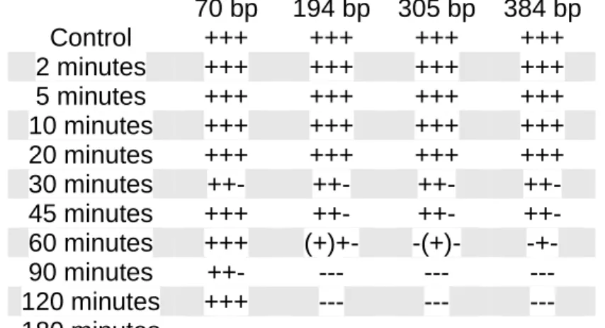
Table 2.1 – Table showing the sequence of the primers used in the 4-Plex multiplex ... 34 Table 2.2 – Table showing the primer volumes added from the 100 µM stock to 28 µL of dH2O in order to make the primer mix for the 4-Plex multiplex ... 34 Table 2.3 – Table showing the PCR cycle conditions for the 4-Plex multiplex .. 35 Table 2.4 – Table showing the parameters employed for the analysis of DNA profiles ... 36 Table 2.5 – Table showing the primers used in the Mini-4-Plex multiplex ... 37 Table 2.6 – Table showing the primer volumes added from the 10 µM stock solution to make the primer mix for the Mini-4-Plex Multiplex ... 37 Table 2.7 – Table showing the PCR cycle conditions for the Mini-4-Plex multiplex ... 38 Table 2.8 – Table showing the cycle conditions for the Primer Extension Reaction ... 38 Table 3.1 – Table showing the primer sequences of amplicons included in the 4-Plex multiplex ... 44 Table 3.2 – Table shows the PCR cycle conditions for the 4-Plex multiplex ... 45 Table 3.3 – Table showing the primer sequences of the Mini-4-Plex amplicons. ... 49 Table 3.4 – Table showing the PCR cycle conditions for the Mini-4-Plex multiplex ... 50 Table 3.5 – Table showing the results of the 4-Plex multiplex amplification for commercial DNA degraded with DNase I. ... 53 Table 3.6 – Table showing the results of the Mini-4-Plex multiplex amplification for commercial DNA degraded with DNase I... 53

(13)

xiii

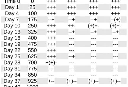
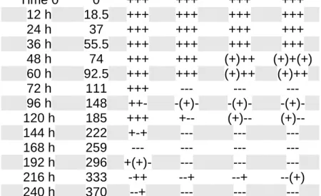
Table 4.1 – Table showing the results of the 4-Plex multiplex amplification for samples incubated at 25 °C. ... 66 Table 4.2 – Table showing the results of the Mini-4-Plex multiplex amplification for samples incubated at 25 °C. ... 68 Table 4.3 – Table showing the results of the 4-Plex multiplex amplification for samples incubated at 37 °C. ... 72 Table 4.4 – Table showing the results of the Mini-4-Plex multiplex amplification for samples incubated at 37 °C. ... 74 Table 4.5 – Table showing the results of the 4-Plex multiplex amplification for samples stored in cell lysis after collection in the field. ... 95 Table 4.6 – Table showing the results of the 4-Plex multiplex amplification for samples stored in ethanol after collection in the field. ... 95 Table 5.1 – Table showing the results of the 4-Plex multiplex amplification for samples stored at room temperature for 7 years using different preservative agents. ... 111 Table 5.2 – Table showing the results of the 4-Plex multiplex amplification for samples stored at -20 °C using different preservation agents ... 121 Table 5.3 – Table showing the results of the 4-Plex multiplex amplification for samples stored at -20 °C and with two cycles of thaw-refreeze using different preservation agents ... 126 Table 5.4 – Table showing the results of the 4-Plex multiplex amplification for samples stored at 25 °C using different preservation agents ... 131 Table 5.5 – Table showing the results of the 4-Plex multiplex amplification for samples stored at 37 °C using different preservation agents ... 133 Table 6.1 – Table showing the results of the 4-Plex multiplex amplification for samples incubated at 25 °C with vacuum. ... 146

(14)

xiv

Table 6.2 – Table showing the results of the 4-Plex multiplex amplification for samples incubated at 25 °C without vacuum. ... 146 Table 6.3 – Table showing the results of the 4-Plex multiplex amplification for samples incubated at 37 °C with vacuum. ... 151 Table 6.4 – Table showing the results of the 4-Plex multiplex amplification for samples incubated at 37 °C without vacuum. ... 151 Table 6.5 – Table showing the results of the 4-Plex multiplex amplification for samples incubated at 37 °C inside bags of three different sizes without vacuum. ... 161 Table 9.1 – International guidelines for human identification ... 197

(15)

xv

LIST OF FIGURES

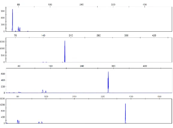
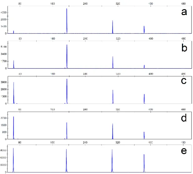
Figure 1.1 – Examples of electropherogram profiles from (a) non-degraded DNA and (b) degraded DNA. ... 8 Figure 1.2 – Diagram showing DNA fragment binding-size range of the columns used. Recoveries of DNA fragments in the size ranges between “removed” and “recovered” are variable. ... 15 Figure 1.3 – Diagram showing schematic of direct and indirect captures of DNA. In the direct capture, the biotinylated DNA bait is incubated with the magnetic beads and immobilized on them. The bead-bait complex is then incubated with the sample for recovery of the target DNA. In the indirect method, the bait is first incubated with the DNA sample and allowed to hybridise. The magnetic beads are added to the bait-target complex, which is immobilized, allowing separation from the rest of the sample. ... 16 Figure 1.4 – Diagram showing the size ranges for some of the analysis methods used for human DNA profiling. SNPs size range was based on SNPforID kit (Sanchez et al. 2006); MiniSTR size range was based on AmpFlSTR®_MiniFiler™ (Horsman-Hall et al. 2009; Mulero et al. 2008); INDEL size range was based on Investigator DIPplex® kit (LaRue et al. 2012); and STR size range was obtained in (Senge et al. 2011). ... 20 Figure 3.1 – Electropherograms of the singleplex amplifications performed with 100 nM stock primers. Some extra peaks appeared, probably due to primer excess. ... 46 Figure 3.2 – Electropherograms of singleplex amplifications performed with 10 nM stock primers. ... 47 Figure 3.3 – Examples of electropherograms of different primer mixes used while trying to balance the 4-Plex multiplex. (a) is the original primer mix; (b-d) are

(16)

xvi

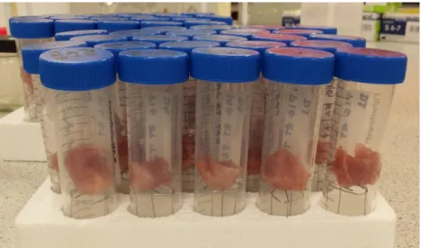
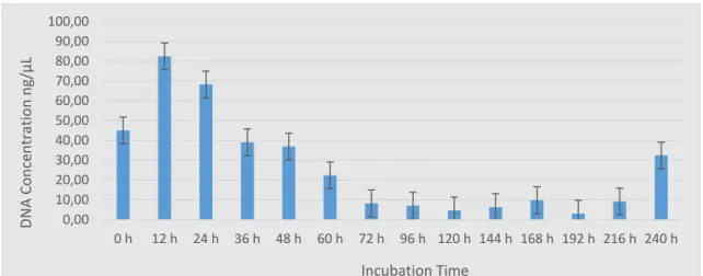
different mixes with varying volumes of the primers; (e) is the new primer mix used with balanced peaks. ... 48 Figure 3.4 – A photograph showing the agarose electrophoresis gel from samples obtained by degrading DNA with DNase I. It is possible to see the smear associated with DNA degradation starting after 2 min of incubation. ... 52 Figure 3.6 –Examples of electropherograms of 4-Plex multiplex profiles obtained from commercial DNA degraded with DNase I. These samples were collected: (a) after 2 min, (b) after 20 min, and (c) after 180 min of incubation and show a full profile, a profile with larger loci affected by degradation and no profile. ... 54 Figure 3.7 – Examples of electropherograms of the Mini-4-Plex multiplex profiles obtained from commercial DNA degraded with DNase I. (a) was degraded for 2 min, and (b) for 60 min. On (c) it is possible to see that some of the amplicons are clear but below the threshold of 50 RFU with 180 min of incubation. ... 54 Figure 4.1: A photograph showing the structure of the polypropylene tubes with muscle samples before incubation. ... 62 Figure 4.2 – A photograph showing the agarose electrophoresis gels from samples incubated at 25 °C at the laboratory. It is possible to see the smear associated with DNA degradation after only 4 days of incubation. Each lane equals to one sample (n=1) but experiments were done in triplicates. ... 64 Figure 4.3 – Bar charts showing the average DNA concentrations of samples incubated at 25 °C at the laboratory from Day 0 to Day 40. The results show no change in Day 1, followed by a peak in Day 4 and subsequently continuous time-dependant decrease in quantitation values. All data are presented as mean ± SEM, n=3. ... 65 Figure 4.4 – Examples of electropherograms of multiplex profiles obtained from samples incubated at 25 °C for (a) 1 day, (b) 7 days, (c) 25 days, (d) 28 days,

(17)

xvii

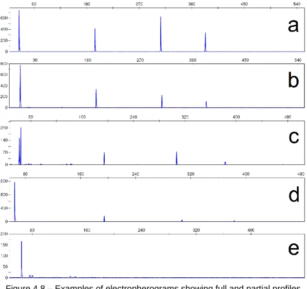
and (e) 37 days. The last image is the sample that presented a profile with clear peaks after 37 days of incubation, even after complete failure of amplification of samples collected at previous time points. ... 67 Figure 4.5 – Electropherograms of some of the samples amplified with the Mini-4-Plex and incubated at 25 °C for (a) 7 days, (b) 22 days, and (c) 37 days. It is possible to see that the profiles get more imbalanced with longer incubation points. ... 68 Figure 4.6 – A photograph showing the agarose electrophoresis gels from samples incubated at 37 °C at the laboratory. It is possible to see the smear associated with DNA degradation in samples stored for as little as 12 h. Each lane equals to one sample (n=1) but experiments were done in triplicates. ... 70 Figure 4.7 – Bar charts showing average DNA concentrations of samples incubated at 37 °C for up to 240 h (10 days). The results show that the quantity of DNA in the samples tended to decrease with time. All data are presented as mean ± SEM, n=3. ... 71 Figure 4.8 – Examples of electropherograms showing full and partial profiles obtained from samples incubated at 37 °C. (a) is the control sample, (b) a sample incubated for 36 h, (c) 120 h of incubation, (d) the sample that after 216 h of incubation amplified 3 of the 4 alleles, and (e) a sample incubated for 240 h. .. 73 Figure 4.9 – Examples of electropherograms of samples incubated at 37 °C and amplified with the Mini-4-Plex. (a) is a sample incubated for 24 h, (b) was incubated for 96 h, and (c) for 240 h. Total amplification was possible even after 10 days of incubation, but the profile is unbalanced and RFUs are low. ... 74 Figure 4.10 – Map showing the location of the city of Nakhon Nayok in relation to Bangkok (116 km apart). ... 79

(18)

xviii

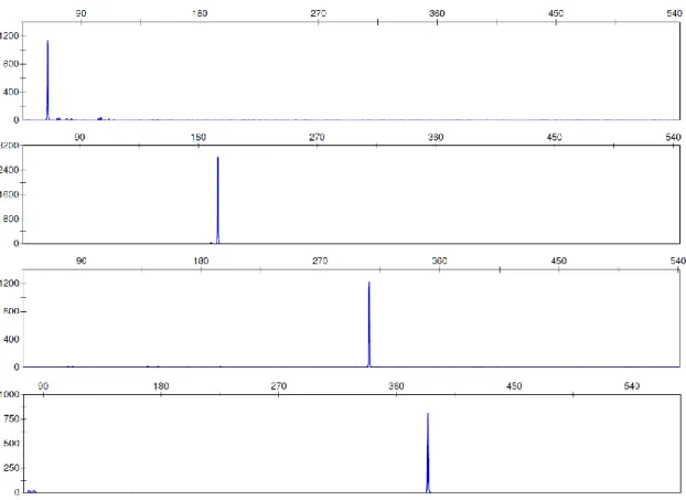
Figure 4.11 – A photograph showing the set-up of the pig carcass and separate limb protected by the mesh cage before the field exposure in Thailand. ... 81 Figure 4.12 – Photograph showing the state of pig carcasses through incubation time points. (a) is a carcass after 12 h of exposure with visible bloating and insect activity on surface; (b) shows insect activity inside previous collection point at 24 h of incubation; (c) to (f) show progressive decomposition and increase of insect activity in carcasses after 36 h, 48 h, 60 h, and 72 h, respectivelly. ... 83 Figure 4.13 – Time course of ambient and internal carcass temperature variations during the three-day-long incubation. The peaks in ambient temperature correspond to noon. ... 84 Figure 4.14 – A photograph showing agarose electrophoresis gel from Thailand samples stored in cell lysis. Each lane equals to one sample. ... 85 Figure 4.15 – A photograph showing agarose electrophoresis gels from Thailand samples stored in ethanol. Each lane equals to one sample. The three first samples in each set of exposed samples were collected from the carcass, followed by one collected from the aerial surface of the separate limb and one from the ground surface of the limb. ... 85 Figure 4.16 – Bar charts showing the DNA concentrations of samples collected in Thailand. Each bar equals to one sample. Some of the samples were not collected in triplicates, so they were not grouped when presenting the results. 94 Figure 4.17 – Examples of electropherograms of full multiplex profile and no multiplex profile obtained from pig muscle stored in cell lysis after sample collection. (a) is a control sample, (b) is a sample collected after 48 h of exposure, and (c) was collected after 60 h of exposure. ... 96 Figure 4.18 – Examples of electropherograms obtained from pig muscle stored in ethanol after collection of sample. It can be observed that the intensity of

(19)

xix

fluorescence decreased between (a) 12 h and (b) 36 h. (c) was collected after 48 h and had no amplification. ... 96 Figure 4.19 – Examples of electropherograms showing that on the two last collection points whilst the samples collected from the aerial surface (a and c) of the limbs had no profile wit RFU levels above 50, the samples collected from the ground surface (b and d) generated complete profiles. ... 97 Figure 5.1 – A photograph showing the agarose electrophoresis gels of pig muscle samples of 0.5 g samples of pig muscle stored at room temperature for 7 years with different preservative agents. Each lane has one sample, but each condition had a triplicate. ... 109 Figure 5.2 – A photograph showing the agarose electrophoresis gels of pig muscle samples of 1 g samples of pig muscle stored at room temperature for 7 years with different preservative agents. Each lane has one sample, but each condition had a triplicate. ... 109 Figure 5.3 – Bar charts showing the average DNA concentrations from samples stored at room temperature for 7 years using different preservative agents. Each bar represents the average of one triplicate of samples. The exception is samples weighting 1 g, incubated for 79 ADD and stored in 96% ethanol, in which the bar represents two samples. Ethanol seems to be more efficient in preserving DNA in the samples. All data are presented as mean ± SEM, n=3. ... 110 Figure 5.4 – Example of electropherograms from samples of this series of experiments. (a) is a sample store in cell lysis; (b) is a sample stored in cell lysis with 1% sodium azide; and (c) is a sample stored in 96% ethanol. All three samples weighted 0.5 g and were exposed for 79 ADD before collection. ... 111 Figure 5.5 – A photograph showing the structure of polypropylene tube with muscle sample and preservative. ... 117

(20)

xx

Figure 5.6 – A photograph showing the agarose electrophoresis gels from samples stored at -20 °C. It is possible to see the smear associated with DNA degradation on the first day of incubation. A clear band associated with high molecular weight DNA is visible in all time points of incubation. Each lane has to one sample and every condition was performed in triplicates. ... 119 Figure 5.7 – Bar charts showing the average DNA concentrations of samples incubated at -20 °C with different preservation agents. The results indicate that 37.5% ethanol is more efficient in preserving DNA in the samples. All data are presented as mean ± SEM, n=3. ... 120 Figure 5.8 – Examples of electropherograms of samples stored at -20 °C, (a) is one sample incubated in 95% ethanol for 1 day; (b) 95% ethanol for 42 days; (c) 37.5% ethanol for 1 day; (d) 37.5% ethanol for 42 days; (e) vodka for 1 day; (f) vodka for 42 days; (g) left untreated for 1 day; (h) left untreated for 42 days. No differences could be observed in the profiles with the increased incubation time, but some degradation is visible at all time points and with all preserving agents. ... 122 Figure 5.9 – A photograph showing the agarose electrophoresis gels from samples stored at --20 °C and with two cycles of thaw-refreeze. It is possible to see the smear associated with DNA degradation beginning on the first day of incubation. A clear band of high molecular weight DNA is visible in all time points of incubation. Each lane has to one sample and every condition was performed in triplicates. ... 124 Figure 5.10 – Bar charts showing the average DNA concentrations of samples incubated at -20 °C with different preservation agents and gone through two thaw-freeze cycles. Again, it seems as 37.5% ethanol was the best preservation solution. All data are presented as mean ± SEM, n=3. ... 125

(21)

xxi

Figure 5.11 – Examples of electropherograms of samples stored at -20 °C and with two cycles of thaw-refreeze. Sample (a) was incubated in 95% ethanol for 1 day; (b) 95% ethanol for 42 days; (c) 37.5% ethanol for 1 day; (d) 37.5% ethanol for 42 days; (e) vodka for 1 day; (f) vodka for 42 days; (g) left untreated for 1 day; (h) left untreated for 42 days. No differences could be observed in the profiles with the increased incubation time. ... 127 Figure 5.12 – A photograph showing the agarose electrophoresis gels from samples at stored 25 °C. On the last day of the incubation, only half of the samples showed high molecular weight DNA bands on the agarose gel. Each lane has to one sample and every condition was performed in triplicates. ... 129 Figure 5.13 – Bar charts showing the average DNA concentrations of samples incubated at 25 °C with different preservation agents. The different conditions seem to have similar DNA concentrations within each time point. All data are presented as mean ± SEM, n=3. ... 130 Figure 5.14 – Examples of electropherograms of samples stored at 25 °C. Sample (a) was incubated in 95% ethanol for 1 day; (b) 95 % ethanol for 42 days; (c) 37.5% ethanol for 42 days; (d) vodka for 42 days; (e) left untreated for 1 day; (f) left untreated for seven days; (g) left untreated for 35 days; (h) left untreated for 42 days. In untreated samples, it is possible to see the decrease of the peak heights of larger amplicons with increased incubation time. ... 132 Figure 5.15 – A photograph showing the agarose electrophoresis gels from samples at stored 37 °C. Samples stored with some kind of preservative agent showed high molecular weight DNA bands up until the last day of incubation while untreated samples only had it present until seven days of incubation. Each lane has to one sample and every condition was performed in triplicates. ... 134

(22)

xxii

Figure 5.16 – Bar charts showing the average DNA concentrations of samples incubated at 37 °C with different preservation agents. Samples left untreated had a peak in DNA quantity on Day 3 and a decrease after that. All data are presented as mean ± SEM, n=3. ... 132 Figure 5.17 – Examples of electropherograms of samples stored at 37 °C. Sample (a) was incubated in 95% ethanol for 1 day; (b) 95 % ethanol for 42 days; (c) 37.5% ethanol for 42 days; (d) vodka for 42 days; (e) left untreated for 1 day; (f) left untreated for 14 days; (g) left untreated for 21 days; (h) left untreated for 35 days. It is possible to see the decrease of the peak heights and drop outs of larger amplicons with a longer incubation time in untreated samples. ... 134 Figure 6.1 – A photograph showing the structure of plastic bag with a piece of pig muscle tissue after vacuum was applied. ... 141 Figure 6.2 – A photograph showing the agarose electrophoresis gels of samples incubated at 25 °C with vacuum at the laboratory. Starting from around day 16 it is possible to see the formation of two clear bands of lower molecular weight DNA. Each lane has one sample, but each condition had a triplicate. ... 144 Figure 6.3 – A photograph showing the agarose electrophoresis gels of control samples incubated at 25 °C in an open tube at the laboratory. DNA was preserved with high molecular weight bands present until the last day of incubation. Each lane has one sample, but each condition had a triplicate. ... 144 Figure 6.4 – Bar charts showing the average DNA concentrations of samples and controls incubated in the laboratory at 25 °C. Samples stored with vacuum had a continuous decrease in the readings while control samples varied more throughout time points. Each bar represents the average of one triplicate of samples. All data are presented as mean ± SEM, n=3. ... 145

(23)

xxiii

Figure 6.5 – Examples of electropherograms of samples and controls incubated at 25 °C. (a) is a time zero sample; (b) is a sample incubated for 13 days with vacuum; (c) is a sample incubated for 40 days with vacuum; (d) is a control incubated for 4 days; (e) is a control incubated for 10 days; (f) is a control incubated for 28 days, and (g) is a control incubated for 40 days. It is possible to see that in samples incubated with vacuum the degradation is slow but progressive, whereas control samples that were air dried did not have a clear pattern of degradation. ... 147 Figure 6.6– A photograph showing the agarose electrophoresis gels of samples incubated at 37 °C with vacuum at the laboratory. Degradation increases with longer incubation times, but high molecular weight DNA is present until the last point of incubation. Each lane has one sample, but each condition had a triplicate. ... 149 Figure 6.7 – A photograph showing the agarose electrophoresis gels of control samples incubated at 37 °C in a bag without vacuum at the laboratory. DNA was less preserved in this set of samples, with more degradation visible. Each lane has one sample, but each condition had a triplicate. ... 149 Figure 6.8 – Bar charts showing the average DNA concentrations of samples and controls incubated in the laboratory at 37 °C. Samples incubated under vacuum had less variation in quantitation readings than control samples incubated without vacuum. Each bar represents the average of one triplicate of samples. All data are presented as mean ± SEM, n=3. ... 150 Figure 6.9 – Examples of electropherograms of samples and controls incubated at 37 °C. (a) is a time zero sample; (b) is a sample incubated for 10 days with vacuum; (c) is a control incubated for 12 h; (d) is a control incubated for 48 h; (e) is a control incubated for 144 h; and (f) is a control incubated for 10 days. .... 152

(24)

xxiv

Figure 6.10 – A photograph showing the different sizes of bags with muscle sample inside them. Bags were sealed with air still inside them. ... 157 Figure 6.11 – A photograph showing the agarose electrophoresis gels of samples incubated in small bags. Each lane is one sample, but each condition had a triplicate. ... 158 Figure 6.12 – A photograph showing the agarose electrophoresis gels of samples incubated in medium bags. Each lane is one sample, but each condition had a triplicate. ... 159 Figure 6.13 – A photograph showing the agarose electrophoresis gels of samples incubated in large bags. Each lane is one sample, but each condition had a triplicate. ... 159 Figure 6.14 – Bar charts showing the DNA quantitation of samples incubated in plastic bags of different sizes at 37 °C. Samples incubated in small bags had less variation in readings than samples incubated in medium and large bags. Each bar represents the average of one triplicate of samples. All data are presented as mean ± SEM, n=3. ... 160 Figure 6.15 – Examples of electropherograms of samples incubated at 37 °C in plastic bags of different sizes. (a) is a time zero sample; (b) is a sample incubated for 2 days in a small bag; (c) is a sample incubated for 10 days in a small bag; (d) is a sample incubated for 2 days in a medium bag; (e) is a sample incubated for 10 days in a medium bag; (f) is a sample incubated for 2 days in a large bag; and (g) is a sample incubated for 10 days in a large bag; n=3.. ... 162 Figure 7.1 – Example of electropherogram from sample degraded for 30 min using DNase I. ... 168 Figure 7.2 – Diagram showing the experimental design of different agarose gel cut methods tried to discover the best yield. ... 169

(25)

xxv

Figure 7.3 – Examples of electrophoresis of (a) the original degraded sample, (b) sample re-extracted after agarose gel electrophoresis. ... 171 Figure 7.4 – Bar charts showing the average DNA recovery of the different combinations of gel cuts. Set A was cut starting from just below the well; and set B was cut with measurements being made around visible DNA in the gel. All data are presented as mean ± SEM, n=3. ... 172 Figure 7.5 – Figure showing the changes in profile observed after DNA gel agarose separation and re-extraction. Red stands for worsening of the profile, yellow for no change observed and green for improvement of the profile. ... 173 Figure 7.6 – Examples of electropherograms of (a) the original degraded DNA sample; (b) sample re-extracted using cut type A2; and (c) sample re-extracted using gel cut type B4 ... 173 Figure 7.7 – Bar charts showing the average DNA recovery of the filtration columns based on DNA incubation time. All data are presented as mean ± SEM, n=3. ... 175 Figure 7.8 – Figure showing the changes in profile observed the use of the purification columns. Red stands for worsening of the profile, yellow for no change observed and green for improvement of the profile... 175 Figure 7.9 Electropherograms of (a) original degraded DNA sample; (b) sample processed with Microcon® DNA Fast Flow Centrifugal Filter Unit column; (c) sample processed with Microcon® 30kDa Centrifugal Filter Unit column; (d) sample processed with illustra MicroSpin G50 column; and (e) sample processed with the MinElute Reaction Cleanup column. ... 176 Figure 8.1 – A schematic diagram showing the Primer Extension Capture reaction. On it, the biotinylated primer and the DNA sample are incubated together and allowed to hybridise. The rest of the DNA strand is formed by the

(26)

xxvi

polymerase. The product of this reaction is then incubated with the magnetic beads and immobilised. Then the rest of the sample is washed away and the sample is heated in order to free the target DNA from the beads. ... 181 Figure 8.2 – Electropherograms of reactions performed with different number of cycles (2 cycles, 5 cycles, 10, cycles, 15 cycles, 20 cycles and 28 cycles) in the Primer Extension step, followed by bead capture and a complete PCR with 30 cycles. ... 184 Figure 8.3 – Electropherograms of half-volume reactions performed with two cycles. Set (a) had all components reduced proportionally to half. Set (b) kept the DNA and primers constant and reduced the buffer volume. ... 184 Figure 8.4 – Electropherogram of DNA Capture reaction where the first step (primer extension) was performed without primers. No amplification occurred later. ... 185 Figure 8.5 – Electropherograms of DNA Capture test runs using (a) the 70 bp and (b) the 384 bp primer pairs. ... 185 Figure 8.6 – Electropherograms of the test reactions combining two primer pairs (70 bp and 194 bp) using (a) two and (b) five cycles for the primer extension step. ... 186 Figure 8.7 – Electropherograms of the same sample with the last step of DNA Capture being (a) the original protocol PCR, showing only the 70 bp amplicon and (b) the 4-Plex Multiplex, showing a complete profile. ... 187 Figure 8.8 – Electropherograms of reactions performed combining the 70 bp and the 384 bp amplicons. (a) was performed with new magnetic beads and the protocol PCR; (b) with reused beads and the protocol PCR; (c) with new magnetic beads and the 4-Plex Multiplex; and (d) with reused beads and the 4-Plex Multiplex. ... 188

(27)

xxvii

Figure 8.9 – Electropherograms of (a) the 70 bp reaction; (b) the 384 bp reaction, and (c) both reactions combined for the last PCR step. ... 189 Figure 8.10 – Electropherogram of a reaction using the 70 bp and the 384 bp primer pairs performed after changing all the reagents used but the magnetic beads. ... 189 Figure 8.11 – Electropherogram of the second test run of the 384 bp primer pair, which resulted in no amplification. ... 190 Figure 8.12 – Electropherograms of single reactions performed with (a) the 70 bp primer pair; (b) the 194 bp primer pair; and (c) the 384 bp primer pair. ... 190 Figure 8.13 – Electropherograms of DNA Capture reactions performed using a combination of the 70 bp and the 384 bp primer pairs (a) with control DNA; (b) is the original degraded DNA sample that was captured in (c). ... 191 Figure 10.1 – Photographs showing two of the body bags that will be used in the field experiments. (a) is a traditional body bag; (b) is the outside of the single-layered body bag, with handles for carrying; (c) is the interior of the same body bag, with absorbent material; (d) is a close-up of the attachment for the pump. ... 231

(28)

xxviii

LIST OF ABREVIATIONS

ADD Accumulated Degree Days

bp Base pairs

CL Cell Lysis

DNA Deoxyribonucleic Acid DNase I Deoxyribonuclease I

ETOH Ethanol

INDEL Insertion/Deletion Polymorphism mtDNA Mitochondrial DNA

MWCO Molecular Weight Cut-Off NGS Next Generation Sequencing PCR Polymerase Chain Reaction PEC Primer Extension Capture

RAG-1 Recombination Activating Gene 1 RAG-2 Recombination Activating Gene 2 RFU Relative Fluorescence Unit

RNA Ribonucleic Acid

SNP Single Nucleotide Polymorphism

STR Short Tandem Repeat

TEG Triethyleneglycol

TRACES Taphonomic Research in Anthropology: Centre for Experimental Studies

(29)

xxix

FINANCIAL ACKNOWLEDGMENT

I would like to thanks CAPES Foundation and the Science Without Borders Program for the student scholarship BEX Process 1308-13/0.

I would like to thanks the ISFG for the Travel Bursary Award for attending the 27th ISFG Conference at Seoul in August, 2017.

(30)

xxx

ACKNOWLEDGMENTS

This work would not have been possible without the help and support of some people that I need to thank.

First, I want to thank my supervisor Dr. William Goodwin for being a centre of calmness and support through this whole process. I also want to say thanks to the FGG team: Dr. Arati Iyengar, Dr. Judith Smith, Dr. Sibte Hadi, and Christine Woodcock (Chrissy), your advice and general help was indispensable.

To the other PhD students that I met during my time at UCLAN, I want to thank you for sharing this journey. I could not have asked for better comrades. Thank you Dina, Haliza, Tundey, Ali, Erum, Pet-Paul, Hussain, Balnd, Eida, and Hayder for the friendship, talks and support.

To my friends back home, who accepted me being absent of almost everything in the past 4 years, a big hug and thank you. Even physically distant, you were always here with me. Cheesy, but true. Thank you De Sempre, Descongela Mas Não Esquenta, NfBR, NICV, and my Hamiltrash friends.

This work would never be finished and this thesis could not have been written without music. I want to thank Lin-Manuel Miranda, Taylor Swift, Cattle & Cane, Muse, Anitta, Chico Buarque, System of a Down, Kate Nash, Morat, Kendrick Lamar, Residente, Shakira, Murray Gold, Yann Tiersen, John Williams, the original casts of Hamilton, Matilda, Waitress, Natasha, Pierre and the Great Comet of 1812, Dear Evan Hansen, and all the Disney composers for providing the soundtrack I needed.

Last but never least, I wish to thank my family, specially my mum and my cousins Talita and Clara. Thank you for dreaming with me about a Christmas in Preston that never happened, for sharing everyday life even though I was not there and for all the jokes and love that make us the best family in the world.

(31)

1

INTRODUCTION

CHAPTER 1

(32)

2

1.1 Forensic Sciences

Forensic sciences are the application of science to criminal and civil laws, as governed by the legal standards of admissible evidence and criminal procedure in each country. They are believed to have started in the 16th century, when medical practitioners in army and university settings began to gather information on the cause and manner of death. Writings in the late 18th century revealed the first evidence of modern pathology. The first school of forensic science was stablished in France in 1909. Since the development of forensic sciences, they have been used to uncover mysteries, solve crimes, and convict or exonerate suspects of crimes.

The field of forensic sciences includes a number of scientific branches, including physics, chemistry, and biology, and focus on the recognition, identification, and evaluation of physical evidence. It has become an essential part of the judicial system, as it utilizes a broad spectrum of sciences to achieve information relevant to criminal and legal evidence. Constant research is of ultimate importance in order to improve methods and aid police officers, courts and families to solve cases and mysteries (AAFS 2014; Jackson and Jackson 2011; Saferstein 2017).

1.2 Decomposition of Post-Mortem Tissues (Cadaveric Decay)

Decomposition will occur when a cadaver is exposed to the environment, with the soft tissue present in the body starting to decay within a few days (Goff 2009). Cadaveric decay is influenced by two destructive processes, namely autolysis and putrefaction (Dent et al. 2004; Janaway et al. 2009).

Autolysis is a process of self-digestion, where the tissues and cells are broken down through the action of intrinsic hydrolytic enzymes (Shirley et al. 2011). Shortly after death, the oxygen supply to cells ceases and the anaerobic

(33)

3

mechanism of glycolysis serves as an alternative energy source in order to maintain basic cellular metabolic activity. This produces waste products such as carbon dioxide and lactate which cause the cellular pH to drop (Swann et al. 2010; Zhou and Byard 2011).

When the cellular membrane can no longer maintain its permeability because of pH difference, it ruptures, releasing cellular contents, including hydrolytic enzymes (Paczkowski and Schuetz 2011). These cellular contents that then act as source of nutrients and energy for the subsequent microbiological activity of the putrefaction process (Zhou and Byard 2011).

Putrefactive breakdown results primarily from the action of bacteria, fungi and protozoa that are already present in the body, mainly in the gastrointestinal tract. These microorganisms digest cellular proteins in local tissue and gain access to the rest of the body via the vascular and lymphatic systems (Dent et al. 2004; Paczkowski and Schuetz 2011).

Exogenous factors affect the rate of cadaveric decay, such as the type of environment and the condition of the body at the moment of death. Ambient temperature and insect activity have great effect on decomposition (Campobasso et al. 2001; Heaton et al. 2014; Ross and Cunningham 2011; Simmons, Adlam et al. 2010; Simmons, Cross et al. 2010). An increase in temperature will accelerate enzymatic reactions and the rate of decomposition, encouraging more oviposition (which is very limited when the temperatures are below 10 °C) and larval development (Prangnell and McGowan 2009). Oxygen availability is also important, with low oxygen levels restricting the microbial activity to anaerobes, thereby slowing the decomposition process (Dent et al. 2004; Statheropoulos et al. 2011).

(34)

4

The cause of death can be one of the main aspects in the speed of cadaveric decay. When bodies have open wounds, the rate of decomposition is much faster than that of a body without any penetrative trauma, principally due to the high prevalence of microorganisms and arthropod oviposition within the wound (Cross and Simmons 2010). In addition, if an individual dies as a result of a viral or bacterial infection, putrefactive post mortem changes are accelerated (Janaway et al. 2009).

A number of facilities that useshuman cadavers in taphonomic research operates in the United States (e.g. the Anthropological Research Facility at the University of Tennessee (Shirley et al. 2011)). For ethical and logistical reasons, body farms have not been in use in the UK. While studies using human cadavers might be preferable due to their direct relevance to forensic cases, as a greater number of animals can be available for use at one study, the use of animal models can facilitate larger studies on the variables that influence decomposition (Cross et al. 2010).

Pigs have been used extensively as an experimental animal model in taphonomic studies, as they have several features that are similar to humans, such as size, anatomy, physiology and metabolic rate (Cross and Simmons 2010; Dekeirsschieter et al. 2009; Myburgh et al. 2013; Simmons, Adlam et al. 2010; Turner and Wiltshire 1999).

1.3 Accumulated Degree Days

In taphonomic studies, decomposition of tissues is regarded as a process that depends more on accumulated temperature rather than time alone. In essence, Accumulated Degree Days (ADD) constitutes of the accumulation of thermal energy needed for the chemical and biological reactions of decomposition to take

(35)

5

place. By using ADD, the energy input into the system is measured as the accumulation of temperature over time.

This cumulative total of daily average temperatures can be used as a quantitative measurement to estimate post-mortem interval. The formula normally used to calculate ADD is the following:

𝐴𝐷𝐷 = 𝑀𝑎𝑥𝑖𝑚𝑢𝑚 𝑇𝑒𝑚𝑝𝑒𝑟𝑎𝑡𝑢𝑟𝑒 + 𝑀𝑖𝑛𝑖𝑚𝑢𝑚 𝑇𝑒𝑚𝑝𝑒𝑟𝑎𝑡𝑢𝑟𝑒

2 − 𝑀𝑖𝑛𝑖𝑚𝑢𝑚 𝑇ℎ𝑟𝑒𝑠ℎ𝑜𝑙𝑑

Where the minimum threshold is the temperature at which biological process stops. In human decomposition studies, the value of 0 °C is commonly used here, since freezing temperatures inhibit most biological processes (Larkin et al. 2010). The use of ADD allows the comparison of studies across multiple and varied environments. Whenever the same amount of thermal energy (ADD) is put into a carcass, the same amount of reaction (body decomposition) will result (Megyesi et al. 2005; Simmons, Adlam et al. 2010).

1.4 DNA Degradation

DNA breakage occurs all the time, but the living organism has repairing enzymes in place to fix it. Upon death, cells and tissues become starved of oxygen and at this point these physiological processes cease to work and decay begins (Demple and Harrison 1994). Depending on several internal and external factors, cells would undergo one of two different death patterns: apoptosis or necrosis. One of these factors is the level of intracellular adenosine triphosphate (ATP). Apoptosis features an energy-dependent programmed cell death where intracellular ATP levels remain unaltered until the very end of the process. Alternatively, necrosis is a passive energy-independent degenerative phenomenon.

(36)

6

Apoptosis usually leads to DNA fragments of around 180 base pairs (bp), with the DNA breaks happening between the nucleosomes. While the ladder-like pattern of oligonucleosomal-sized fragments in agarose electrophoresis is produced as a hallmark of apoptosis, the random digestion characteristic of necrosis creates the smear associated with degraded DNA (Alaeddini et al. 2010).

In early necrosis, endonuclease-mediated DNA cleavage is characterized by selective generation of 5’ overhangs. Endogenous endonucleases will cleave the DNA around the histone structure (the most vulnerable sections) and this generates fragments of 300 kb (rosette structure) or 50 kb (loop structure). After digestion of the chromatin proteins, random digestion by the endonucleases will occur, with the rate of degradation depending on temperature, pH levels, and expression level of the enzymes (Didenko et al. 2003; Golenberg et al. 1996; Paabo et al. 2004). Changes towards necrosis occur faster in higher ambient temperatures and necrosis is typically induced by extremes in the external environmental conditions of the cell (such as hypoxia), or through the action of membrane active toxicants and respiratory poisons (Alaeddini et al. 2010). There are also non-enzymatic processes that are present and responsible for DNA breakdown, which happen much slower, but should not be ignored. Some of them are more likely to happen in muscle tissue than others, but the DNA can be subjected to any of them in an uncontrolled environment.

Denaturation involves the unwinding of the double helix structure, due to breakages in the hydrogen bonds that hold the DNA strands together. Although the nucleotide sequence remains unchanged, denaturation increases the susceptibility to other types of chemical attack (Lindahl and Nyberg 1974). Cross-linking happens when one of the strands of the double helix become chemically

(37)

7

bonded to other molecules. Similar to denaturation, nucleotides are unchanged, but cross-linking can interfere with analyses (Brown 1999).

Hydrolic reactions will attack the glycosidic base–sugar bond and the hydrolysis of DNA is enhanced by the presence of water, resulting in strand breakages, base loss and chemical modifications to the nucleotide units (Lindahl and Karlstro 1973). Chemical modifications can involve the addition, removal or replacement of a chemical group on a nucleotide. These modifications can change the entire nucleotide sequence. Strand breakages occur where there are breaks in the sugar phosphate backbone of the DNA, causing the whole molecule to fragment (Brown 1999).

Oxidative damage can change sugar residues, remove bases and create strand breakages and cross-linkage (Epe et al. 1993; Lindahl 1993). Lastly, radiation can create oxidative damage, strand breaks, modification of bases, and formation of dimers (Alaeddini et al. 2010; Hoss et al. 1996; Overballe-Petersen et al. 2012; Paabo et al. 2004).

Highly degraded DNA samples will typically display poor amplification of the larger sized alleles when using standard short tandem repeat (STR) multiplex typing kits. Because of how degradation works, the amplification and profiling of shorter amplicons is more successful in degraded templates due to the fact that lower molecular weight loci are more likely to stay intact (Butler et al. 2003; Dixon et al. 2006; Takahashi et al. 1997).

As STR amplicon sizes in commercial multiplex kits used for DNA identification are usually between 100 bp and 450 bp, degraded samples will generate at least an imbalanced DNA profile. In this case, the larger amplicons fall below the detection limits, and a partial genetic profile can be seen (Cotton et al. 2000; Greenspoon et al. 2006; Krenke et al. 2002). A decay curve can be seen in

(38)

8

multiplex kits with a wide range of amplicon sizes, where the peak height is inversely proportional to the amplicon length (Lygo et al. 1994; Wallin et al. 1998). In more degraded samples, the longer alleles can drop out completely, leaving the profile incomplete (Figure 1.1) (Chung et al. 2004; Hughes-Stamm et al. 2011; Senge et al. 2011; Westen et al. 2009).

With increased degradation levels, polymerase chain reaction (PCR) artefacts such as preferential amplification, allele drop out and locus drop out become more common (Bender et al. 2004; Foran 2006; Lindahl 1993).

Figure 1.1 – Examples of electropherogram profiles from (a) non-degraded DNA and (b) degraded DNA.

1.5 Tissue Preservation

The International Criminal Police Organization (INTERPOL) recommends friction ridge analysis, dental analysis and DNA analysis as primary methods of identification (INTERPOL 2014). Following mass fatality incidents and in some crime scenes, human corpses are disassembled, burnt or decomposed, making victim identification by means of fingerprinting or odontology extremely difficult. In such situations, DNA analysis can play a crucial role; however, successful DNA analysis from post-mortem samples relies heavily on the appropriate collection and preservation of biological material (Graham et al. 2008). The DNA

(39)

9

Commission of the International Society for Forensic Genetics says that storing soft muscle tissue samples in preservative solutions at room temperature can be an alternative to cold storage (Prinz et al. 2007).

Tissue type is one of the principal factors affecting DNA preservation. Bone and teeth have resilient structures which slow DNA degradation, especially when compared to soft tissue samples. However, the process of DNA extraction from hard tissues is laborious and time consuming (Budowle et al. 2005; Dawson et al. 1998).

The rate of DNA degradation is variable amongst soft tissue samples. Bär et al. (1988) studied samples from brain cortex, lymphatic node, liver, spleen, psoas muscle, kidney, thyroid gland, and blood with post-mortem ages varying between 6 h and 19 days. Complete DNA degradation was observed in liver tissue after 24 h, while spleen, kidney and thyroid gland showed good DNA stability up to 5 days. Another study by Larkin et al. (2010) was able to amplify a fragment of 200 bp from muscle samples collected from pig carcasses exposed for up to 10 days in the winter. Samples of rat brain, kidneys, liver and skeletal muscle of the thigh collected up to 6 weeks after death were analysed with real-time PCR. The results show that the brain had the most DNA persistence, followed by muscle (Itani et al. 2011).

In forensic genetics, tissue preservation is usually connected with disaster victim identification (McNevin 2016) and preservation methods should be able to generate a profile using commercial kits. Inefficient preservation methods can lead to the breakdown of intact DNA to such an extent that data are not always available for victim identification (Bing and Bieber 2001). Biological samples have been successfully preserved using a number of physical and chemical

(40)

10

treatments, adjusting temperature, ambient pH and salt concentrations (Dawson et al. 1998).

1.5.1 Temperature

Sample storage at -20 °C enhances DNA preservation (Budowle et al. 2005). Hara et al. (2016) investigated DNA degradation from blood stains over a range of temperatures from -80 C up to room temperature. Temperatures below -20 °C preserved DNA better and temperatures above 4 °C significantly degraded the DNA when compared to all other temperatures.

The impact of freeze-thaw cycles of whole blood samples on DNA integrity in the sample was previously studied (Bellete et al. 2003; Gessoni et al. 2004; Krajden et al. 1999; Ross et al. 1990) and the results showed progressive degradation of the samples as the number of freeze-thaw cycles increased. Freeze-thaw cycles would be expected to be equally detrimental to the stability of DNA in soft tissues, as ice crystals grow upon freezing, which speed up the breakdown of cell membranes, leading to accelerated autolysis.

1.5.2 Preservation Solutions

Cell lysis (CL) solutions have been used to preserve soft muscle tissue samples for different periods of time (Allen-Hall and McNevin 2013). Lysis storage and transportation buffer was used to preserve 5-100 mg of muscle tissue at room temperature and complete STR profiles were obtained for up to 12 months (Graham et al. 2008). Lysis buffer was used to preserve liver tissue for up to 2 years. No DNA could be extracted from tissue after 2 years of storage, but high molecular weight DNA was recoverable from the buffer solution (Kilpatrick 2002). Alcohol storage is considered to be an effective long term tissue storage method that allows for successful DNA extraction from preserved specimens (Penna et

(41)

11

al. 2001). Ethanol (ETOH) has been used previously for the preservation of specimens at room temperature (Gillespie et al. 2002; Kilpatrick 2002; Michaud and Foran 2011). It is cost-effective and readily obtained, making it an attractive candidate for field applications. King and Porter (2004) investigated the effect of a range of alcohol concentrations from 70-100% on DNA preservation in ant specimens, noting that a concentration of 95-100% was most effective. They reported that ethanol was preferred over other alcohols due to faster penetration of cell membranes and a better ability to deactivate deoxyribonuclease (DNase) activity.

The use of vodka in the preservation of zebra liver samples over several days in the African Bush was reported by Oakenfull (1994). It was found that the DNA extracted after using this method was not as high quality as those samples stored in ethanol or methylated spirits; however, the DNA produced was still satisfactory for amplification.

1.5.3 Vacuum Preservation of Tissues

Vacuum was the first technology applied to packaging methods used commercially in the food industry. It consists of removing the air from the package, thus creating an anoxic environment. Due to the lack of oxygen, bacterial microflora is selected and growth of aerobic microorganisms is hindered, whereas anaerobic and facultative bacteria grow slowly. Vacuum preservation diminishes the growth of the microbial community when compared to aerobic preservation methods (Bellés et al. 2017).

Spoilage of raw meat is a combination of biological and chemical activities, but is mainly caused by microbial metabolic activity. The initial microbial community is influenced by storage conditions, such as the temperature and the packaging environment (Casaburi et al. 2015; Jääskeläinen et al. 2016). Vacuum packaging

(42)

12

reportedly diminishes the spoil of products like fruits, vegetables and various kinds of meat (Araujo et al. 2017; Bouletis et al. 2017; Costa et al. 2016; Hernández, E. J. G. P. et al. 2017; Jin et al. 2017; Lee et al. 2016; Li et al. 2017; Lloret et al. 2016; Sergio et al. 2016; T. Wang et al. 2016; Yang et al. 2016). Biobanks and hospitals are also looking at vacuum preservation in order to reduce or cease to use formaldehyde (Condelli et al. 2014). In one study Di Novi et al. (2010) found that under-vacuum sealing of tissues preserved gross anatomic features better than formalin, improved histological features in solid organs, facilitated gene expression profiling of breast cancer specimens, and preserved RNA, thus permitting tissue banking and gene expression profiling. Bussolati et al. (2008) found that the absence of air decreased autolytic processes, and increased protein and RNA stability. The stability of RNA tends to be shorter than that of DNA, but no studies were found analysing DNA persistence when storing muscle tissue samples with vacuum.

1.6 DNA Extraction

DNA extraction in forensic laboratories is a crucial step in the workflow. Since all following procedures depend on it, then it is important to extract as much DNA as possible (good yield) and it must be of good quality, with no inhibitors. The selection of technique must adapt so that each sample is treated accordingly. Some of the current used protocols are FTA Paper, Chelex 100, organic extraction, and silica-based extraction (Bogas et al. 2014).

FTA paper extraction is a simple method for reference samples. The sample is applied to the FTA card, which has chemicals in it that cause cell lysis. The released DNA binds to the paper. Extraction is based on washing steps to remove non-DNA material.

(43)

13

The use of Chelex 100 is quite common in crime samples. The resin protects the DNA during the heating process of the extraction by binding to divalent ions such as Mg2+_{ions that are a required co-factor to DNases. But besides this technique} not being able to remove inhibitors, since Mg2+_{ions are needed in the} amplification reaction, Chelex itself can inhibit following steps (Phillips et al. 2012).

Organic extraction produces a cleaner DNA when compared with Chelex 100 extraction, but it requires the use of phenol, which potentially causes health problems because of its toxic nature. The protocol starts with lysing the material, followed by washing steps with a phenol-chloroform mixture and DNA purification (Carpi et al. 2011).

Traditional silica-based extraction protocols already showed better results than Chelex and organic extraction (Phillips et al. 2012). Combining silica-based techniques with magnetic beads, a silica-coated magnetic bead extraction was created. In this extraction, the samples go through salting-out and the free DNA binds to the beads. Using a magnetic separator and several washing steps, the DNA is cleaned and then released from the beads (Witt et al. 2012).

The method of choice for extracting DNA in degraded samples varies depending of the tissue and the decomposition stage. Studies have shown that the low copy number associated with degraded samples may be originated from the low retention rates of small fragments in extraction methods (Barta et al. 2014).

1.7 DNA Size Separation of DNA Molecules

Sample purification is included in the routine of most laboratories in order to remove inhibitors. Purification can also be used post-amplification in order to remove excess primers and other reagents. In this research, purification columns

(44)

14

were used as a way to remove small fragments of degraded DNA from samples prior to amplification. As proof of the concept that it is possible to preferentially select DNA fragments of different sizes, agarose gel electrophoresis was used. 1.7.1 Agarose Gel Electrophoresis

Agarose gel electrophoresis is a relatively easy and fast method to assess the quality of DNA. This technique also allows the user to recover DNA intact from a band and individually isolate fragments. Agarose is a polymer that when mixed with an electrophoresis buffer forms a porous matrix that acts like a net for the DNA. When an electric current is applied, smaller fragments pass through the “net” more easily than bigger fragments, which are retained. High molecular weight DNA can be seen as a single band on the top of the gel while degraded DNA appears as a smear (Goodwin et al. 2007; Phillips et al. 1998).

1.7.2 Purification Columns

Some purification columns were chosen for their application in removal of small molecules and fragments of DNA from samples. They have different size cutouts (Figure 1.2) and utilise different techniques in order to achieve this goal.

Microcon® centrifugal filters can be used for concentration, desalting or buffer exchange of aqueous biological samples. The anisotropic, hydrophilic membranes in Microcon® centrifugal filter devices are characterized by either a molecular weight cut-off (MWCO) or a performance-specific application (e.g., DNA recovery). MWCO is the ability of the membrane to retain molecules above a specified molecular weight, and this retention depends on the molecular size and shape of the solutes. Moreover, solutes with molecular weights close to the MWCO may be only partially retained.

(45)

15

The illustra MicroSpin G-50 Columns purify DNA by the process of gel filtration with the use of Sephadex™ G-50 DNA grade F resin. This column is designed for rapid purification of DNA and it is suitable for recovery of any DNA fragment larger than 20 bp, but will not remove or denature enzymes. The gel filtration process works by penetration of the matrix by the molecules applied. Product retention is inversely relative to molecular size, as the size increases, the retention decreases. Molecules larger than the pores in the Sephadex™ are excluded, and intermediate sized molecules penetrate the matrix to varying extents, depending on size. Small molecules have complete penetration, which retards the process through the column.

The MinElute DNA Cleanup column uses a silica membrane combined with spin-column technology, meaning that it has the selective binding capacities of one along with the convenience of the other. DNA is applied to the silica membrane and absorbed in the presence of high concentrations of salt while contaminants pass through the column. Impurities are washed away and the DNA is eluted. DNA purified with this technique is suitable for any subsequent application.

Figure 1.2 – Diagram showing DNA fragment binding-size range of the columns used. Recoveries of DNA fragments in the size ranges between “removed” and

(46)

16

1.8 Magnetic Beads-Based DNA Capture

DNA hybridization capture is a DNA purification method that allows for the separation of the targeted DNA loci from the rest of the DNA in the sample. Magnetic-bead DNA separation is commonly used for total DNA non-specific purification (Wang and McCord 2011). It has been incorporated in automated DNA extraction protocols (Archer et al. 2006; Haak et al. 2008; Nagy et al. 2005; Rittich and Spanova 2013; Witt et al. 2012) where the beads bind to non-specific DNA in order to separate it from inhibitors and contaminants.

There are different approaches that can be used for DNA capture and they can be divided into two groups, namely indirect and direct capture (Figure 1.3). The main difference between them is that in the direct capture, hybridization occurs in a solid phase (immobilised), while the indirect capture has its hybridization in solution.

Figure 1.3 – Diagram showing schematic of direct and indirect captures of DNA. In the direct capture, the biotinylated DNA bait is incubated with the magnetic beads and immobilized on them. The bead-bait complex is then incubated with the sample for recovery of the target DNA. In the indirect method, the bait is first

incubated with the DNA sample and allowed to hybridise. The magnetic beads are added to the bait-target complex, which is immobilized, allowing separation