Cost-Optimal Execution of Boolean DNF Trees with Shared Streams

Shared Streams

Henri Casanova, Lipyeow Lim, Yves Robert, Fr´

ed´

eric Vivien, Dounia Zaidouni

To cite this version:

Henri Casanova, Lipyeow Lim, Yves Robert, Fr´

ed´

eric Vivien, Dounia Zaidouni. Cost-Optimal

Execution of Boolean DNF Trees with Shared Streams. [Research Report] RR-8616, INRIA.

2014.

<

hal-01079868v2

>

HAL Id: hal-01079868

https://hal.inria.fr/hal-01079868v2

Submitted on 11 Dec 2014

HAL

is a multi-disciplinary open access

archive for the deposit and dissemination of

sci-entific research documents, whether they are

pub-lished or not.

The documents may come from

teaching and research institutions in France or

abroad, or from public or private research centers.

L’archive ouverte pluridisciplinaire

HAL

, est

destin´

ee au d´

epˆ

ot et `

a la diffusion de documents

scientifiques de niveau recherche, publi´

es ou non,

´

emanant des ´

etablissements d’enseignement et de

recherche fran¸cais ou ´

etrangers, des laboratoires

publics ou priv´

es.

0249-6399 ISRN INRIA/RR--8616--FR+ENG

RESEARCH

REPORT

N° 8616

Cost-Optimal Execution

of Boolean DNF Trees

with Shared Streams

Henri Casanova, Lipyeow Lim, Yves Robert, Frédéric Vivien, and

Dounia Zaidouni

RESEARCH CENTRE GRENOBLE – RHÔNE-ALPES

Inovallée

655 avenue de l’Europe Montbonnot

Trees with Shared Streams

Henri Casanova

_{, Lipyeow Lim}

_{, Yves Robert}

_{, Frédéric}

Vivien

_{, and Dounia Zaidouni}

Research Report n° 8616 — December 2014 — 53 pages

Abstract: Several applications process queries expressed as trees of Boolean operators applied to predicates on sensor data streams, e.g., mobile apps and automotive apps. Sensor data must be retrieved from the sensors, which incurs a cost, e.g., an energy expense that depletes the battery of a mobile device, a bandwidth usage. The objective is to determine the order in which predicates should be evaluated so as to shortcut part of the query evaluation and minimize the expected cost. This problem has been studied assuming that each data stream occurs at a single predicate. In this work we study the case in which a data stream occurs in multiple predicates, either when each predicate references a single stream or when a predicate can reference multiple streams. In the single-stream case we give an optimal algorithm for a single-level tree and show that the problem is NP-complete for DNF trees. For DNF trees we show that there exists an optimal predicate evaluation order that is depth-first, which provides a basis for designing a range of heuristics. In the multi-stream case we show that the problem is NP-complete even for single-level trees. As in the single stream case, forDNFtrees we show that there exists a depth-first leaf evaluation order that is optimal and we design efficient heuristics.

Key-words: query processing, boolean operators, energy, scheduling, greedy algorithm, data sharing

∗_{University of Hawaii at M¯anoa, HI, USA} †_{École normale supérieure de Lyon, France}

‡_{LIP laboratory – CNRS, ENS Lyon, INRIA, UCB Lyon 1} §_INRIA

partageant des données

Résumé : Le traitement de requêtes, exprimées sous forme d’arbres d’opérateurs booléens appliqués à des prédicats sur des flux de données de senseurs, a de nombreuses applications dans le domaine du calcul mobile. Les données doivent être transférées des senseurs vers l’appareil de traitement des données, ce qui induit un coût, par exemple une consommation énergétique qui diminue la charge des batteries, ou une utilisation de bande passante. L’objectif est de déterminer l’ordre dans lequel les prédicats doivent être évalués de manière à court-circuiter une partie de l’évaluation de l’arbre et de minimiser l’espérance du coût. Ce problème a déjà été étudié sous l’hypothèse que chaque flux apparaît dans un seul prédicat. Dans le présent travail nous étudions le cas où un flux peut être utilisé par plusieurs prédicats, soit quand chaque prédicat référence un unique flux (cas mono-flux), soit quand un prédicat peut référencer plusieurs flux (cas multi-flux). Dans le cas mono-flux, nous donnons un algorithme optimal pour les arbres à un seul niveau et nous montrons que le problème est NP-complet pour les arbres sous forme normale disjonctive (FND). Pour les arbres FND nous montrons qu’il existe un ordre optimal d’évaluation des prédicats qui est en profondeur d’abord; cette propriété nous sert à proposer toute une gamme d’heuristiques. Dans le cas multi-flux, nous montrons que le problème est NP-complet même pour les arbres à un seul niveau. Comme dans le cas mono-flux, nous montrons qu’il existe un ordre d’évaluation des prédicats en profondeur d’abord qui est optimal et nous proposons des heuristiques efficaces.

Mots-clés : traitement de requêtes, opérateurs booléens, énergie, ordonnancement, algorith-mique probabiliste, algorithme glouton, partage de données

OR AND l3:C <3 l1:AVG(A,5)<70 l2:MAX(B,4)>100 (a) AND AND OR

AVG(A,5)<70 MAX(B,4)>100 C <3 MAX(A,10)>80

(b) AND OR MIN(B,7)<MAX(A,10) AVG₍A,5)<70 AVG(B,10)>10 (c)

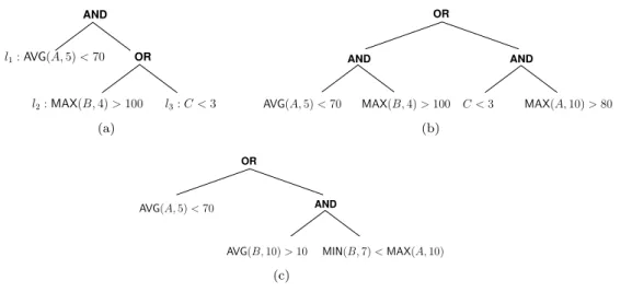
Figure 1: Three query tree examples: (a) a read-once query; (b) ashared query in the single-streamcase; (c) a shared query in themulti-stream case.

1

Introduction

An increasing number of applications are being developed or envisioned that continuously pro-cess data generated via sensors embedded in or associated with mobile devices. Smartphones are equipped with increasingly sophisticated sensors (e.g., GPS, accelerometer, gyroscope, micro-phone) that enable near real-time sensing of an individual’s activity or environmental context. A smartphone can then perform embedded query processing on the sensor data streams for, e.g., social networking [1], remote health monitoring [2]. Automotive applications running on a smartphone can acquire data from sensors in a vehicle (e.g., engine status, speed, angular speed) as well as from remote databases (e.g., weather, traffic, road works) so as to perform continuous queries that trigger appropriate responses (e.g., alerting the driver that driving conditions are dangerous) [3].

In the above applications there is a cost associated to the acquisition of sensor data. Even moderate data rates can cause commercial smartphone batteries to be depleted in a few hours [4]. In the automotive application scenario, the acquisition of sensor data incurs a cost in terms of bandwidth usage on the sensor network in the vehicle [3]. Consequently, solutions must be developed to reduce the cost of sensor data acquisition when processing continuous queries.

In this work we study the problem of minimizing the (expected) cost of sensor data acquisition when evaluating a query expressed as a tree of conjunctive and disjunctive Boolean operators applied to Booleanpredicateson the data. Each predicate is computed over data items from dif-ferent data streams generated periodically by sensors, and has a certain probability of evaluating to true. The evaluation of the query stops as soon as a truth value has been determined, possibly

shortcircuiting part of the query tree. A “push” model by which sensors continuously transmit data to the device maximizes the amount of acquired data and is thus not practical. Instead, a “pull” model has been proposed [5], by which the query engine carefully chooses the order

and the numbers of data items to acquire from each individual sensor. This choice is based on a-priori knowledge of operator costs and probabilities, which can be inferred based on historical traces obtained for previous query executions. Such intelligent processing is possible thanks to the programming and data filtering capabilities that are emerging on sensor platforms [6, 3].

which produce integer data items. Each leaf corresponds to a Boolean predicate. A predicate may involve no operator, e.g., “C <3” is true if the last item from stream C is strictly lower than 3, or based on an arbitrary operator (in this exampleMAX_,MIN_{, or}AVG_{) which is applied}

to a time-window for a stream, e.g., “AVG_{(A,5)<70” is true if the average of the last 5 items}

fromAis strictly lower than 70), or multiple operators (e.g., “MIN_(B,7)<MAX_(A,10)”).

Most results in the literature are forread-oncequeries, i.e., when each data stream occurs in at most one leaf of the query tree. The example query tree in Figure 1(a) is aread-once query since no stream occurs in two leaves. In this work we study the more general case, which we termshared, in which a stream can occur in multiple leaves. Figure 1(b) shows ashared query in which streamAoccurs at two leaves. Such queries are easily envisioned in most domains. For instance, in a telehealth example, an alert may be generated either if the heart rate is high and the acceleration is zero or if the heart rate is low and the SPO2 (blood oxygen saturation) is low.

Sharedqueries relevant to an automotive application are considered in [3]. We also study the case in which multiple streams can occur in a single predicate. An example is shown in Figure 1(c), in which streamsAandB occur in multiple leaves, and together in one leaf. We term the scenarios in Figure 1(a) and 1(b)single-stream and the scenario in Figure 1(c)multi-stream.

Considering shared queries has important algorithmic implications that we explore in this work. The device that processes the query acquires data items from streams and holds each data item in memory until the query has been processed. Each time a leaf of the query must be evaluated, one can then compute the number of data items that must be retrieved from the relevant stream given the time-windows of the operators applied to that stream and the data items from that stream that are already in the device’s memory. For example, considering the query in Figure 1(b), assume the predicate “AVG_{(A,5)<70” is evaluated first, thus acquiring 5}

items from streamA. If later the predicate “MAX_{(A,10)>80” needs to be evaluated then only}

5 additional items must be acquired.

In this work we study theshared queries and make the following contributions: • ForANDquery trees:

– We give a polynomial-time greedy algorithm (which is not as straightforward as the optimal algorithm forread-oncequeries) that is optimal in thesingle-streamcase, and show that the problem in NP-complete in themulti-stream case.

– For the multi-streamcase we propose an extension of the single-stream greedy algo-rithm. This extension is not optimal but computes near-optimal leaf evaluation orders in practice.

• ForDNFquery trees:

– We show that the problem is NP-complete in thesingle-streamcase (and thus also in themulti-streamcase).

– In both thesingle-streamandmulti-streamcase we show that there exists an optimal leaf evaluation order that is depth-first;

– We develop heuristics that we evaluate in simulation and compare to the optimal solution (computed via an exhaustive search on small instances) and to the single-streamheuristic proposed in [5].

Section 2 discusses related work. Section 3 defines the problem and our assumptions formally. Section 4 gives a method for computing the expected cost of a leaf evaluation order. We then study the problem forANDtrees andDNFtrees in Section 5 and Section 6, respectively, for both thesingle-stream and multi-streamcases. Section 7 concludes the paper with a brief summary of our findings and perspectives on future work. The source code and data for all experiments are publicly available1_.

2

Related work

The problem of computing the truth value of a Boolean query tree while incurring the mini-mum cost is known as ProbabilisticAND-ORTree Resolution (PAOTR) and has been studied extensively in the literature.

Forread-once queries the complexity of the PAOTR problem is unknown for generalAND -OR trees. Smith et al. [7] propose a simple O(nlogn) greedy algorithm (n is the number of leaves in the query tree) that produces an optimal leaf evaluation order for AND trees (i.e., single-level trees with an AND operator at the root node). Greiner et al. [8] survey known theoretical results and present several new results. They consider a depth-first approach that recursively replaces rooted subtrees with a single equivalent single node. They show that this approach can be arbitrarily sub-optimal for trees with 3 levels or more. For DNF trees (i.e., collections ofANDtrees whose roots are the children of a singleORnode), they show that this approach is dominant, meaning that there is always one optimal strategy that corresponds to a depth-first traversal. They proposed aO(nlogn) depth-first traversal of the tree that reuses the algorithm in [7] to order leaves within each AND, which produces an optimal evaluation order for anyDNFtree.

Shared queries, the focus of this work, are important in practice and have been introduced and investigated by Lim et al. [5]. In that work the authors do not give theoretical results, but instead develop heuristics to determine an order of operator evaluation that hopefully leads to low data acquisition costs. To the best of our knowledge, the complexity of the PAOTR problem for shared queries has never been addressed in the literature, likely because re-using stream data across leaves dramatically complicates the problem. When picking a leaf evaluation order, interdependences between the leaves must be taken into account. In fact, even when given a leaf evaluation order, computing the expected query cost is intricate while this same computation is trivial forread-once queries.

Several problems studied in the literature are closely related to the PAOTR problem and fall in the area of system testing [9], and in particular the evaluation of priced functions [10] and the Discrete Function Evaluation Problem (DFEP) [11].

Charikar et al. [10] and Cicalese et al. [12] study the evaluation of “priced functions.” In this context an algorithm seeks to read a subset of the function’s inputs so that the function’s output can be determined with minimum price. When the function is anAND/ORtree there exist algorithms that achieve the best possible competitive ratio in pseudo-polynomial [10] and polynomial [12] time. In this context, no knowledge of the Boolean variables (which correspond to our predicates) is assumed. In the context of our work this would correspond to all predicates having the same probability of success of 1

2. However, ignoring probabilities of success can lead to solutions that are no better thanL-competitive for functions withLinputs, even for a single AND tree2_.

Cicalese et al. [11] have studied the Discrete Function Evaluation Problem (DFEP). An instance of DFEP is defined by a set S of objects, a partition C of these objects into classes (which represent the values taken by the function), a probability distributionponS, a setT of tests, and a cost function assigning a cost to each test. The goal of DFEP is to design a testing procedure that uses tests from T to identify the class that includes the unknown object, while 2_{Consider anANDnode with}Lleaves of unit cost,L−1 having a probability of success of 1−ǫand the last

one having a probability of success ofǫ. If theǫ-probability leaf is evaluated first the expectation of the cost of the

evaluation of the query is 1 +ǫ(1 + (1₋ǫ)(1 + (1₋ǫ)(...+ (1₋ǫ)1))) = 1 +ǫ((1₋ǫ)0+ (1₋ǫ)1+...+ (1₋ǫ)L−2_{) =}

1 + (1−(1−ǫ₎L−1_{) ≈ 1 + (}L₋₁₎ǫ _when ǫ _{tends to zero. When probabilities are ignored, all leaves are}

absolutely equivalent and a probability-agnostic leaf evaluation order can evaluate the ǫ_{-probability leaf last,}

leading to a leaf evaluation order with expected cost equal to: 1 + (1−ǫ)(1 + (1−ǫ)(1 +...(1 + (1−ǫ)(1)))) =

(1−ǫ)0+ (1₋ǫ)1+...+ (1₋ǫ)L−1₌ 1−(1−ǫ)L

minimizing the expectation of the testing cost (or the worst-case testing cost). DFEP has also been studied under the names of the Equivalence Class Determination problem [13] and of the Group Identification problem [14].

Evaluation of AND/ORtrees is a special case of DFEP where the set of objects is the set of the possible instantiations of the vector of predicates, where the probability distribution is the probability of occurrences of the different instantiations, where there are only two classes corresponding to instantiations leading to the AND/OR tree evaluating to True or False, and where tests correspond to the evaluation of predicates. There exist approximation algo-rithms for the minimization of the expectation of the testing cost with ratioO(log(|S|)) [11] or Olog 1

pmin

[13, 14], wherepminis the minimum probability of an object (pmin= mins∈Sp(s)).

ForAND/ORtrees,|S|= 2L _andp

min≤ 1₂

L

. Therefore, all these approximations algorithms are O(L)-approximation algorithms forAND/OR tree evaluation. However, for single-stream

AND/OR trees without reuse where all costs are identical (what is often called the uniform case), any schedule is aO(L)-approximation if theAND/ORtree is neither a tautology nor a false statement: in the best case at least one predicate must be evaluated, and in the worst case allLpredicates must be evaluated. Therefore, existing results for DFEP do not lead to efficient solutions for theAND/ORtree evaluation problem.

3

Problem statement / Framework

A query is anAND-ORtree, i.e., a rooted tree whose non-leaf nodes areANDorORoperators, and whose leaves are labeled with probabilistic Boolean predicates. Each predicate is evaluated over data items generated by datastreams. The evaluation of each predicate has a knownsuccess probability, i.e., the probability that the predicate evaluates toTRUE. In practice, the success probability can be estimated based on historical traces obtained from previous query evaluations. As in [8], we assumeindependentpredicates, meaning that two predicates at two leaves in a query are statistically independent. Evaluating a predicate incurs has acostdetermined by the number of data items required to perform the evaluation and a per data item cost for the stream. For instance, the cost of a data item could correspond to the energy cost, in joules, of acquiring one data item based on the communication medium used for the stream and the data item size.

More formally, we consider a set of streams, S = {s1, . . . , sS}. Stream sk has a cost per

data item of c(sk). A query on these streams, T, is a rooted AND-OR tree with L leaves

L={l1, . . . , lL}. Leaflj has success, resp. failure, probabilitypj, resp. qj = 1−pj, and requires

the lastdsk

lj items from each streamsk∈ S. d

sk

lj is zero iflj does not require items fromsk. The

objective is to compute the truth value of the root of the query tree by evaluating the leaves of the tree. Because each non-leaf node is either anOR or an AND operator, it may not be necessary to evaluate all the leaves due toshortcircuiting. In other words, as soon as any child node of an OR, resp. AND, operator evaluates to TRUE, resp. FALSE, the truth value of the operator is known and can be propagated toward the root. For a given query, we define a schedule as an evaluation order of the leaves of the query tree, represented as a sorted leaf sequence.

We define thecost of a schedule as theexpected valueof the sum of the costs incurred for all leaves that are evaluated before the root’s truth value is determined. For instance, consider the query in Figure 1(a), in which leaves are labeledl1, l2, l3, and consider the schedulel2, l3, l1. Query processing begins with the acquisition of the data items necessary for evaluatingl2, which has cost 4·c(B). With probabilityp2,l2evaluates toTRUE, thus shortcircuiting the evaluation ofl3. Therefore, the expected evaluation cost of theORoperator is: 4·c(B) +q2·c(C). If the ORoperator evaluates toFALSE, which happens with probabilityq2q3, then the evaluation of

l1 is shortcircuited. Otherwise, l1 must be evaluated. The overall cost of the schedule is thus: 4·c(B) +q2·c(C) + (1−q2q3)·5·c(A). Recall that this query tree corresponds to aread-once query.

The PAOTR problem consists in determining a schedule with minimum cost. Forread-once

queries the complexity of PAOTR is unknown for general AND-ORquery trees, while optimal polynomial-time algorithms are known forANDtrees [7] and DNFtrees [8]. In this work, we focus on these two types of trees as well but forshared queries.

4

Evaluation of a schedule

Our overall objective is to study the problem of computing an optimal schedule for ANDand DNFtrees forshared queries. First, in this section we explain how the expected cost of a given schedule can be computed. This computation is non-trivial, as seen on an example (Section 4.1), but can be performed in polynomial time (Section 4.2).

4.1

Schedule evaluation example

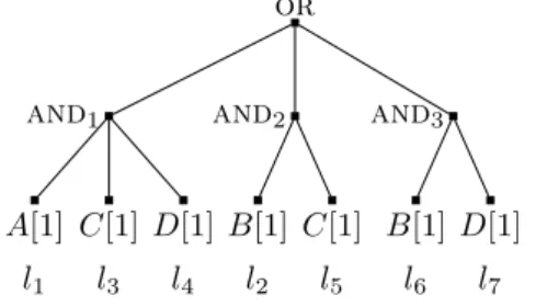
In this section, we illustrate on an example what is involved when computing the expected cost of a schedule. Consider theDNFtree in Figure 2 with threeANDnodes, for four streamsA,B, C, andD. For each leaf we indicate how many data items it requires from each stream and its probability of success. In this example each leaf requires a single data item from a stream. Since each leaf requires data items from a single stream this tree corresponds to thesingle-streamcase. We provide a (more complex) example for the multi-streamcase in A. Leaves are labeled l1 to l7, in the order in which they appear in a given schedule. Computing the cost of a schedule is much more complicated than forread-once queries due to inter-leaf dependencies. LetCj be the

cost of evaluating leaflj, andCthe overall cost of the schedule. We consider the 7 leaves one by

one, in order:

Leaf l1 –The first leaf is evaluated: C1=c(A).

Leaf l2 –This is the first leaf in itsAND, noAND has been fully evaluated so far, andl2 is the first encountered leaf that requires streamB. Therefore, l2 is always evaluated, requiring a data item from streamB: C2=c(B).

Leafl3 –This is the second leaf from itsAND, noANDhas been fully evaluated so far, andl3 is the first encountered leaf that requires stream C. Therefore, a data item fromC is acquired if and only ifl1 evaluates toTRUE: C3=p1c(C).

Leaf l4 –This is the third leaf from itsAND, noANDhas been fully evaluated so far, andl4 is the first encountered leaf that requires streamD. Therefore, one data item is acquired from D if and only ifl1andl3 both evaluate toTRUE: C4=p1p3c(D).

Leaf l5 – This is the second leaf from its AND, and AND1 has been fully evaluated so far. However, one of the leaves of thatAND,l3, requires a data item that is also needed byl5, from streamC. Ifl3has been evaluated, then the evaluation cost ofl5is 0 because the necessary data item fromC has already been acquired and is available “for free” when evaluating l5. Ifl3 has not been evaluated (with probability 1−p1), it means that AND1 has evaluated to FALSE. Then, if l2 has evaluated to TRUE, l5 must be evaluated thus requiring the data item from streamC. We obtainC5= (1−p1)p2c(C).

Leaf l6 –Since l2 is always evaluated the data item from stream B required by l6 is always available for free: C6= 0.

Leafl7–This is the second leaf from itsAND, andAND1andAND2have been fully evaluated so far. However, one of the leaves of AND1, l4, but none of those of AND2, requires the data item that is needed by l7 from streamD. Therefore, l7 must be evaluated and its evaluation

or

and1 and2 and3

A[1] l1 C[1] l3 D[1] l4 B[1] l2 C[1] l5 B[1] l6 D[1] l7 Figure 2: Examplesingle-stream DNFtree.

is not free if and only if l4 has not been evaluated, AND2 has evaluated to FALSE, and the evaluation ofAND3 went as far asl7. Therefore,C7= (1−p1p3)(1−p2p5)p6c(D).

Overall, we obtain the cost of the schedule:

T C = c(A) +c(B) + (p1+ (1−p1)p2)c(C) + (p1p3+ (1−p1p3)(1−p2p5)p6)c(D). Given the complexity of the above cost computation on a small example, one might expect the PAOTR problem to be NP-complete forsharedqueries (recall that it is polynomial forread-once

queries). We confirm this expectation in Section 6.

4.2

Schedule evaluation algorithm

Consider aDNF tree with N AND nodes, indexed i = 1, . . . , N. As defined in Section 3 the set of leaves is denoted byL and has cardinality L. To capture the structure of theDNF tree we modify the leaf notation in Section 3 as follows. ANDnodeihasmi leaves, denoted byli,j,

j = 1, . . . , mi. The probability of success of leaf li,j is denoted by pi,j. The query is over S

streams, ss, s = 1, . . . , S and each leaf can require data from multiple streams as in the more

general multi-stream case. The cost per data item of ss is denoted by c(ss). We define the

“t-th data item” of a stream as the data item produced t time-steps ago, so that the first data item is the one produced most recently, the second is the one produced before the first, etc. In this manner, when we say that leafli,j requiresds_li,js data items from streamss it means that it

requires allt-th data items of the streamssfort= 1,2, . . . , ds_li,js . Finally, we consider a schedule

ξ, which is an ordering of the leaves, and use lr,t ≺lu,v to indicate that leaf lr,t occurs before

leaflu,v inξ.

Given the above, we define Ls,t as the set of the leaves that require the t-th data item

from streamssand that are the first of their respective ANDnodes to require that data item.

Formally, we have: Ls,t= n li,j∈ L d ss li,j ≥t, and (∀r6=j, d ss

li,r < tor li,j≺li,r)

o .

We also defineAi,j, the index set of all ANDnodes that have been fully evaluated before leaf

li,j is evaluated, as:

Ai,j={k|mk =|{lk,r|lk,r≺li,j}|}.

If we useCli,j,s,t to denote the expected cost of retrieving thet-th data item of streamss when

evaluating leafli,j, then the total costC of the scheduleξis:

C= X li,j∈ξ    S X s=1 dss li,j X t=1 Cli,j,s,t   . (1)

The following proposition givesCli,j,s,t.

Proposition 1. Given a leaf li,j that does not require the t-th data item from streamss, then

Cli,j,s,t= 0. Otherwise, if there existsrsuch thatli,r ≺li,j andli,r∈ Ls,t, thenCli,j,s,t= 0, else:

Cli,j,s,t = Y lr,v∈Ls,t lr,v≺li,j  1− Y lr,u≺lr,v pr,u   × Y a∈Ai,j 6∃r, la,r∈Ls,t 1− ma Y r=1 pa,r ! ×   Y li,u≺li,j pi,u  ×c(ss).

Proof. Consider a scheduleξ, a streamss, and an integert. Consider a leaf in that schedule,li,j,

which requires thet-th data item from streamss. Let us prove the first part of the proposition.

If leaf li,j does not require the t-th data item from stream ss, then the acquisition cost is 0.

Otherwise, if a leafli,r (i.e., a leaf in the sameANDnode asli,j) occurs beforeli,jinξ(li,r≺li,j)

and requires thet-th item from streamss(i.e.,li,r ∈ Ls,t), then there are two possibilities. Either

li,r has been evaluated, in which case the evaluation of li,j uses a data item that has already

been acquired previously, hence a cost of 0. Or li,k has not been evaluated, meaning that its

evaluation was shortcircuited. In this case the AND node has evaluated to FALSE and the evaluation ofli,j is also shortcircuited and the cost is 0.

The second part of the proposition shows the expected cost as a product of three factors, each of which is a probability, and a fourth factor,c(ss), which is the cost of acquiring the data

item from the stream. The interpretation of the expression forCli,j,s,t is as follows: a leaf must

acquire thet-th item from streamssif and only if (i) the item has not been previously acquired;

and (ii) no AND node has already evaluated to TRUE; and (iii) no leaf in the same AND node has already evaluated toFALSE. We explain the computation of these three probabilities hereafter.

The first factor is the probability that none of the leaves that precedeli,jinξand that require

thet-th item from streamsshave been evaluated. Such a leaflr,sis evaluated if all the leaves in

the sameAND node that precede it in the schedule have evaluated toTRUE, which happens with probabilityQ

lr,u≺lr,spr,u. Hence, the expression for the first factor.

The second factor is the probability that none of theANDnodes that have been fully eval-uated so far has evaleval-uated toTRUE, since if this were the case the evaluation ofli,j would not

be needed, leading to a cost of 0. Given an AND node inAi,j, say the k-th AND node, the

probability that it has evaluated toTRUEisQmk

r=1pk,r. This is true except if one of the leaves

of thatANDnode belongs toLs,t. The first factor assumes that that leaf was not evaluated and,

therefore, that that entire ANDnode was not evaluated. Hence, the expression for the second factor.

The third factor is the probability that all the leaves in the sameANDnode asli,j that have

been evaluated have evaluated toTRUE. Because we are in the second case of the proposition, none of these leaves requires thet-th item of streamss. All these leaves must evaluate toTRUE,

otherwise the evaluation ofli,jwould be shortcircuited, for a cost of 0. Hence, the expression for

the third factor.

The expected cost of a scheduleξcan be computed from Eq. (1) and Proposition 1. We now derive the complexity of carrying out this computation. Recall that L is the total number of

and A[1] 0.75 l1 A[2] 0.1 l2 B[1] 0.5 l3

Figure 3: Exampleshared ANDtree for which the read-oncealgorithm in [7] is not optimal.

leaves in the tree. LetDbe the maximum number of required data items over all streams. More formally,L=PN

i=1mi andD= max1≤i≤N,1≤j≤midli,j. To compute all the setsLs,twe need to

scan the leaves of eachANDnode according to scheduleξwhile recording the maximum number of items required from each stream. This can be done with complexity O(L). Each set Ls,t

contains at mostN leaves. Computing all the setsAi,j is also done through a traversal of the set

of leaves, for an overall cost ofO(L+N2_{) (because the setsA}

i,j take at mostN distinct values

and each contains at mostN elements). Computing all the product of probabilities used in the computation of all theCli,j,s,t can also be done in a single traversal of the set of leaves. Once all

these precomputations are done, the first term in the expression ofCli,j,s,t can be computed in

O(N), the second inO(N2_{), and the third one inO(1). We computeC}

li,j,s,t for all the streams

required by the leaf li,j and the maximum number of streams required by a leaf is S. Overall

the cost of a schedule can be evaluated with complexity

O(LSDN2_).

5

AND trees

In this section we focus onANDtree forsharedqueries. We first show that the optimal algorithm forread-oncequeries is no longer optimal forsharedqueries (Section 5.1). We develop an optimal greedy algorithm in the single-stream case (Section 5.2). We show that the problem is NP-complete in themulti-streamcase, for which we propose a heuristic that we show to be close to the optimal for small instances (Section 5.3).

5.1

Is the optimal

read-once

algorithm still optimal?

One valid question is whether the algorithm in [7], which is optimal for read-once queries, is still optimal for shared queries. It turns out that it is not, and in this section we provide a counter-example. Consider theAND tree depicted in Figure 3 with three leaves labeledl1,l2, and l3, for two streams A and B. For each leaf (li), we indicate the stream, the number of

data items needed from that stream to evaluate the leaf, and the success probability (pi). For

instance, leafl2 requiresdAl2 = 2 items from stream Aand evaluates toTRUEwith probability

p2 = 0.1. We assume that retrieving a data item from any stream has unitary cost. There are 6 possible schedules for this tree, each schedule corresponding to one of the 3! orderings of the leaves. The algorithm in [7] sorts the leaves by non-decreasingds

ljc(s)/qj, wheres is the only

stream from whichlj requires data items. Because 1×_qc₁(A) =₁₋1_0.75 = 4, 2×_qc₂(A) =₁₋2_0.1 ≈2.22,

and 1×_qc₃(B) = 1

1−0.5 = 2, this algorithm schedules leaf l3 first. There are two possible schedules withl3 as the first leaf:

• l3, l1,l2 whose cost is: c(B) +p3×(c(A) +p1×c(A)) = 1 + 0.5×(1 + 0.75×1) = 1.875; and

• l3,l2,l1whose cost is: c(B) +p3×(2×c(A) +p2×0×c(A)) = 1 + 0.5×(2 + 0.1×0) = 2. However, another schedule,l1,l2,l3, has a lower cost: c(A) +p1×(c(A) +p2×c(B)) = 1 + 0.75× (1 + 0.1×1) = 1.825. Therefore, the optimal algorithm for the PAOTR problem forread-once

ANDtrees is no longer optimal forshared ANDtrees.

5.2

The

single-stream

case

In this section we give an optimal algorithm for solving the problem forshared ANDtrees in the

single-stream case. Like the algorithm in [7] forread-once queries, our algorithm is greedy. But it compares the ratios of cost to failure probability of all sequences of leaves that use the same stream, instead of only considering pair-wise leaf comparisons. We begin with a preliminary result on the optimal ordering of leaves that use the same stream.

5.2.1 Ordering same-stream leaves

In the example given in Section 5.1 we consider two schedules that begin with leafl3. In the first schedule leafl1precedesl2, while the converse is true in the second schedule. Leafl1requires one data item from streamA, while leafl2requires two data items from the same stream. Therefore the first schedule is always preferable to the second schedule: if we evaluate l1 beforel2 and if l1 evaluates to FALSE, then there is no need to retrieve the second data item and the cost is lowered. A general result can be obtained:

Proposition 2. Consider an AND tree and a leaf li that requires dsli >0 data items from a stream s. In an optimal schedule, li is scheduled before any leaf lj that requires ds_lj > ds_li data

items from stream s.

Proof. This proposition is proven via a simple exchange argument (see B).

5.2.2 Optimal schedule

Consider an AND tree with L leaves, l1, . . . , lL, for S streams, s1, . . . , sS. We define Lk =

{lj | dsljk > 0}, i.e., the set of leaves that require data items from stream sk. We propose a

greedy algorithm,SingleStreamGreedy(Algorithm 1). This algorithm, which is implemented recursively for clarity of presentation, takes as input theLk sets, an initially empty scheduleξ,

and an array of S integers,NumItems, whose elements are all initially set to zero. This array is used to keep track, for each stream, of how many data items from that stream have been retrieved in the schedule so far. Each call to the algorithm appends to the schedule a sequence of leaves that require data items from the same stream, in increasing order of number of data items required. The algorithm stops when all leaves have been scheduled. The algorithm first loops through all the streams (thekloop). For each stream, the algorithm then loops over all the leaves that use that stream, taken in increasing order of the number of items required. For each such leaf the algorithm computes the ratio (variableRatio) of cost to probability of failure of the sequence of leaves up to that leaf. The leaf with the minimum such ratio is selected (leaf lj0 in

the algorithm, which requiresdsk0

lj0 data items from streamsk0). In the last loop of the algorithm,

all unscheduled leaves that requiredsk0

lj0 or fewer data items from streamsk0 are appended to the

schedule in increasing order of the number of required data items.

Theorem 1. SingleStreamGreedyis optimal for thesharedPAOTR problem forANDtrees. Proof sketch. We prove the theorem by contradiction. We assume that there exists an instance for which the schedule produced by SingleStreamGreedy, ξgreedy, is not optimal. Among

Algorithm 1:SingleStreamGreedy({L1, ...,LS}, ξ,NumItems) 1 if ∪S i=1Li=∅then returnξ 2 MinRatio←+∞ 3 fork= 1 toS do 4 Cost ←0 5 Proba←1 6 Num←NumItems[k] 7 forl_j ∈ L_k by non-decreasing dsk lj do

8 Cost ←Cost+Proba×(dsk

lj −Num)×c(k) 9 Proba←Proba×p_j 10 Num←dsk lj 11 Ratio← Cost (1−Proba)

12 if Ratio<MinRatio then 13 MinRatio←Ratio 14 j₀←j;k₀←k 15 forl_j inL_k 0 by non-decreasing d sk0 lj do 16 if dsk0 lj ≤d sk0 lj0 then 17 ξ←ξ · l_j 18 L_k 0 ← Lk0\ {lj} 19 NumItems[k₀]←dsk0 lj0

20 returnSingleStreamGreedy({L1, ...,L_S}, ξ,NumItems)

the optimal schedules, we pick a schedule,ξopt, which has the longest prefix Pin common with ξgreedy. We consider the first decision taken by SingleStreamGreedy that schedules a leaf that does not belong toP. Let us denote bylσ(1), ..., lσ(k) the sequence of leaves scheduled by this decision. The first leaves in this sequence may belong to P. LetP′ be P minus the leaves lσ(1), ...,lσ(k). Then,ξgreedy can be written as:

ξgreedy=P′, lσ(1), ..., lσ(k),S.

In turn,ξopt can be writtenξopt =P′,Q,Rwhere lσ(k) is the last leaf ofQ. In other words,Q can be writtenL1, lσ(1), ..., Lk, lσ(k), where each sequence of leavesLi, 1≤i≤k, may be empty.

We can write:

ξopt=P′, L1, lσ(1), ..., Lk, lσ(k),R. Fromξgreedyandξopt, we build a new schedule,ξnew, defined as

ξnew =P′, lσ(1), ..., lσ(k), L1, ..., Lk,R.

P′_{, l}

σ(1), ..., lσ(k) is a prefix to bothξgreedy andξnew. This prefix is strictly larger thanPsince Pdoes not contain lσ(k). We compute the cost of ξnew and show that it is no larger than that ofξopt, thus showing thatξnew is optimal and has a longer prefix in common withξgreedy than ξnew, which is a contradiction. This computation is lengthy and technical and the full proof is provided in C.

40000 Cost 60 40 20 0

Shared instances sorted by increasing optimal cost 120000 80000

0

Algorithm in [7] Optimal algorithm

Figure 4: Cost achieved by the algorithm in [7] and that achieved by the optimal SingleStream-Greedyalgorithm, for 157,000 randomANDtree instances sorted by increasing optimal cost.

The complexity ofSingleStreamGreedyisO(L2_{). Indeed, the setsL1, ...,L}

Sare built and

sorted inO(Llog(L)) time and there are at most Lrecursive calls toSingleStreamGreedy, each having a cost proportional to the number of leaves remaining in theANDtree.

One may wonder how the optimal algorithm for read-once queries [7], which simply sorts the leaves by increasingds

ljc(s)/qj, fares forshared queries. In other terms, is

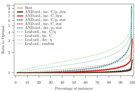
SingleStream-Greedyreally needed in practice? Figure 4 shows results for a set of randomly generatedAND trees. We define the sharing ratio, ρ, of a tree as the expected number of leaves that use the same stream, i.e., the total number of leaves divided by the number of streams. For a given number of leaves L = 2, . . . ,20 and a given sharing ratio ρ = 1,5/4,4/3,3/2,2,3,4,5,10, we generate 1,000 random trees for a total of 157,000 random trees (note thatρ cannot be larger than the number of leaves). Leaf success probabilities, numbers of data items needed at each leaf, and per data item costs are sampled from uniform distributions over the intervals [0,1], [1,5], and [1,10], respectively. For each tree we compute the cost achieved by the algorithm in [7] and that achieved by our optimal algorithm. Figure 4 plots these costs for all instances, sorted by increasing optimal cost. Due to this sorting, the large number of samples, and the limited resolution, the set of points for the optimal algorithm appears as a curve while the set of points for the algorithm in [7] appears as a cloud of points. These results show that the algorithm in [7] can lead to costs up to 1.86 times larger than the optimal. It leads to costs more than 10% larger for 19.54% of the instances, and more than 1% larger for 60.20% of the instances. The two algorithms lead to the same cost for only 11.29% of the instances. We conclude that, for shared

queries,SingleStreamGreedyprovides substantial improvements over the optimal algorithm forread-once queries.

5.3

The

multi-stream

case

In this section, we first show the NP-completeness of determining the optimal schedule for a

multi-streamANDtree. Next we show how to extend the greedy algorithm of thesingle-stream

case. While no longer optimal, this extended greedy algorithm is close to the optimal in practice and thus proves useful for designing heuristics.

5.3.1 The multi-stream case is NP-complete

Definition 1(AND-Multi-Decision). Given a multi-streamANDtree and a cost boundK, is there a schedule whose expected cost does not exceedK?

Theorem 2. AND-Multi-Decisionis NP-complete.

Proof. The problem is clearly in NP: given a schedule, i.e., an ordering of the leaves, one can compute its expected cost in polynomial time (using the method given in Section 4) and compare it toK. The NP-completeness is obtained by reduction from 2-PARTITION [15]. LetI1 be an instance from 2-PARTITION: given a set{a1, ..., an}andS=Pni=1ai, does there exist a subset

I such that P

i∈Iai = S₂? We assume thatS is even, otherwise there is no solution. The size

ofI1 is O(n×logM), whereM = max1≤i≤n{ai}. Without loss of generality, we assume that

M ≥10. We construct the following instanceI2 of AND-Multi-Decision:

• We consider an AND tree with n+ 1 leaves ℓi, 1 ≤ i ≤ n+ 1. The set of streams is

S ={A1, . . . , An, B}. The cost of streamsi =Ai fori≤nisc(i) = ₂1_Z, whereZ is some

large constant defined hereafter. The cost of stream sn+1 =B is c(n+ 1) = C0, where C0≈1₂ is a constant defined hereafter.

• The firstnleaves have a single stream: for 1≤i≤n, leafℓiaccesses 2aielements of stream

Ai, so that the cost of evaluating leaf ℓi (without re-use) is a_Zi. The success probability of

leafℓi is pi= 1− ai Z −β a2 i Z2, whereβ ≈1

2 is a constant defined hereafter.

• Leafℓn+1 accesses alln+ 1 streams: one element of the streamB, andai elements of each

of the nstreams Ai. The cost of evaluating leaf ℓn+1 (assuming no re-use of data items acquired during the evaluation of other leaves) is C = C0+Pn_i=12a_Zi = C0+₂S_Z. The success probability of leaf ℓn+1 is pn+1 = ε. Constantε is chosen to be very small, see below. Intuitively,Cwould be the cost of a schedule evaluating leafℓn+1first, and thereby terminating the evaluation, whenεbecomes negligible.

• The bound on the expected evaluation cost isK=C1−₈S_Z22

+ 1

9Z2.

To finalize the description ofI2, we define the constants as follows: • Z = 10 (n+ 1)3n_+n3 M3_, • C0=_2ZZ_−S −₂S_Z, so thatC=_2ZZ_−S, • β= 1−C 2C , • ε= 1 (n+1)2_90Z2.

The size ofI2 is polynomial in the size ofI1: the greatest value inI2 is Z and log(Z) is linear in (n+ logM). BecauseZ is very large relatively toS≤nM, we do have thatC,C0, andβ are all close to 1

2. We only use that these constants are all nonnegative, and thatβ≤1 andC≤1, in the following derivation, where we bound the expected cost of an arbitrary evaluation of the ANDtree. Then, using this derivation, we prove thatI1 has a solutionI if and only ifI2 does. Let us start with the cost of an arbitrary evaluation of theANDtree. In such an evaluation, we evaluate some (possibly none) of the firstnleaves before evaluating leafℓn+1. Then, because

εis small, we can compute an approximation of the cost as follows: we assume that the schedule terminates after leaf ℓn+1, because its success probability is close to 0. We will bound the difference between this approximation and the actual cost later on.

LetI ={ℓσ(1), ℓσ(2), . . . , ℓσ(k)} be the subset, of cardinal k, of leaves that are evaluated, in

that order, before leafℓn+1. LetCost be the approximated cost of the schedule (terminating after completion of leaf ℓn+1). To simplify notations, we let xi =aσ(i) andri =pσ(i) for 1≤i≤k. By definition: Cost = k X i=1 xi Z Y 1≤j<i rj+ C− k X i=1 xi 2Z ! Y 1≤j≤k rj.

Note that the cost of leafℓn+1 has been reduced from its original value, due to the sharing of the streams whose index is inI. To evaluate Cost, we start by approximating

Y 1≤j<i rj = Y 1≤j<i 1−xj Z −β x2 j Z2 ! . Let Fi= 1− i−1 X j=1 xj Z −β i−1 X j=1 x2 j Z2 + X 1≤j1<j2<i xj1xj2 Z2 . We have   Y 1≤j<i rj  −Fi ≤ 3 n_M3 Z3 . (2)

To see this, we have kept inFiall terms of the productQ1≤j<irj whose denominators include a

factor strictly inferior toZ3_{. The other terms of the product are bounded (in absolute value) by} M3_/Z3_{, becauseβ≤1,x}

j ≤M, andM ≤Z. There are at most 3i−1≤3n such terms. Hence

the desired bound in Equation (2). Letting

G= k X i=1 xi Z − X 1≤j1<j2≤k xj1xj2 Z2 , we prove similarly that

  k X i=1 xi Z Y 1≤j<i rj  −G ≤ n3 n_M3 Z3 . (3)

Indeed, there are k≤n terms in the sum, each of them being bounded as before. We deduce from Equations (2) and (3), usingC≤1, that

Cost− G+ (C− k X i=1 xi 2Z)Fk+1 ! ≤(n+ 1)3 n_M3 Z3 . (4)

Now, we aim at simplifyingH =G+ (C−Pk

i=1 2xZi)Fk+1 by dropping terms whose denominator

isZ3_{. We have} H = k X i=1 xi Z − X 1≤j1<j2≤k xj1xj2 Z2 + C− k X i=1 xi 2Z ! 1− k X j=1 xj Z −β k X j=1 x2 j Z2 + X 1≤j1<j2≤k xj1xj2 Z2  .

Defining ˜ H=C+1−2C 2Z k X i=1 xi+ 1 2Z2 k X i=1 xi !2 +C−1 Z2 X 1≤j1<j2≤k xj1xj2− βC Z2 k X i=1 x2 i,

we derive (usingβ≤1) that:

H−H˜ ≤ 1 2Z3 k X i=1 xi !  X 1≤j1<j2≤k xj1xj2+ k X i=1 x2i   . Hence, H−H˜ ≤ n3_M3 Z3 . (5) Developing (Pk i=1xi)2=Pki=1x2i + 2 P 1≤j1<j2≤kxj1xj2 in ˜H, we obtain ˜ H=C+1−2C 2Z k X i=1 xi+ C Z2 X 1≤j1<j2≤k xj1xj2+ 1−2βC 2Z2 k X i=1 x2i.

We have chosen the constantsCandβ so that ˜H can be reduced to

˜ H =C+ C 2Z2   S 2 − k X i=1 xi !2 −S 2 4  . (6) Indeed, we have 1−2C 2Z = −SC

2Z2, and C = 1−2Cβ. Altogether, we derive from Equations (4)

to (6) that Cost−C 1− S 2 8Z2 − C 2Z2 S 2 − k X i=1 xi !2 ≤ (n+ 1)3 n_+n3 M3 Z3 = 1 10Z2. (7)

Finally, we coarsely bound the difference between the actual cost Cost of the schedule and the approximated cost Cost. The actual probability of evaluating some other leaves after leaf ℓn+1 is ε, there are at most nsuch leaves, whose individual cost does not exceed ₂M_Z. We get a difference bounded bynM

2Zε, from which we derive

Cost−Cost ≤n M 2Zε≤(n+ 1) 2_ε= 1 90Z2. (8)

We could easily tighten the bound in Equation (8), but we will keep the same notations to derive a similar bound in the proof of Theorem 4.

Combining Equations (7) and (8), we finally derive that Cost−C 1− S 2 8Z2 − C 2Z2 S 2 − k X i=1 xi !2 ≤ 1 9Z2. (9)

We now prove that I1 has a solution I if and only if I2 does. Suppose first that I1 has a solutionI: P

ℓn+1, followed by the remaining leaves in any order. Let Cost be the cost of this evaluation. From Equation (9), we have

Cost−C 1− S 2 8Z2 ≤ 1 9Z2. Hence,Cost≤C1− S2 8Z2 + 1

9Z2 =K, thereby providing a solution toI2.

Suppose now thatI2has a solution whose cost isCost≤K, and letIdenote the (index) set of leaves that are evaluated before leaf ℓn+1. If (by contradiction) we have P_i∈Iai 6= S₂, then

S 2 − Pk i=1xi 2

≥1, and Equation (9) shows that

Cost ≥C 1− S 2 8Z2 + C 2Z2− 1 9Z2 =K+ 9C−4 9Z2 . Since 9C−4 = Z+4S

2Z−S, 9C−4>0. Then,Cost > K and we obtain a contradiction. Therefore

P

i∈Iai =S2, andI1 has a solution, which concludes the proof.

5.3.2 Greedy heuristic for themulti-stream case

SinceAND-Multi-Decision is NP-complete we propose a greedy scheduling heuristics, Mul-tiStreamGreedy (Algorithm 2), which extends the ideas of SingleStreamGreedy to the

multi-streamcase.

SingleStreamGreedy computes a schedule by concatenating sequences of leaves. Each such sequence consists of leaves that all require data items from the same stream. These leaves are ordered by non-decreasing number of required data items. We extend this approach to the

multi-stream case thanks to a notion of dominance. We say that leafli dominates leaf lj if for

each streamsleaflirequires at least as many data items fromsaslj(dsli ≥d

s

lj).

MultiStream-Greedyconsiders all sequences of yet-to-be-scheduled leaves such that the (i+ 1)-th leaf in the sequence dominates the i-th leaf. Like SingleStreamGreedy, MultiStreamGreedy picks the sequence that has the lowest ratio of cost to probability of failure.

Consider an AND tree with a set of leaves L = l1, . . . , lL. MultiStreamGreedy takes

L as input and returns a schedule, ξ, and its expected cost. While there remain leaves to schedule (while loop at line 6), MultiStreamGreedy computes all dominance relationships among the yet to be scheduled leaves via a call to DirectDomination (Algorithm 6 in D). DirectDominationreturns the set of source leaves, i.e., leaves that dominate no other leaves (boolean arraySource), and the set of dominance relationships (boolean arrayDominates). These relationships are direct, i.e., not including transitive dominances. For each source leafli,

Multi-StreamGreedythen examines all possible sequences starting withli(for loop at line 11). This

is done via a call to the recursiveGreedyKernelfunction (Algorithm 3), which computes the sequence that starts with li that provides the best extension to the current schedule.

Multi-StreamGreedythen selects the best extension among all these extensions for all source leaves (lines 14-18).

The complexity of GreedyKernelisO(2L_{). This is because GreedyKernelexplores all}

paths starting from a given source leaf in the dominance relationship graph (in a directed acyclic graph with nvertices there are at most O(2n_{) paths). MultiStreamGreedy has complexity}

O(L2₂L_{). This is because at each step MultiStreamGreedy schedules at least one leaf and}

calls GreedyKernelfor each unscheduled source leaf. In spite of its exponential worst-case complexity, for the problem instances used in our experimental evaluations we are able to execute

GreedyKernelin at most 0.03 sec (for aANDnode with 40 leaves) on one core of an 2.1 GHz AMD Opteron processor.

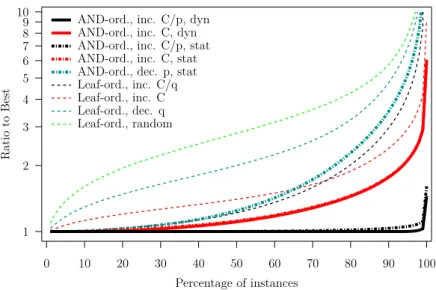
Figure 5 shows results for a set of randomly generatedANDtrees. Instances are generated using the same method as that described in Section 5.2.2. For a given number of leaves L = 2, . . . ,10 and a given sharing ratio ρ = 1,5/4,4/3,3/2,2,3,4,5,10, we generate 1,000 random trees for a total of 81,000 random trees. The number of streams referenced by each leaf is sampled from a uniform distribution over the interval [1,5], and each such stream is sampled uniformly from the set of streams. For each tree we compute the cost achieved byMultiStreamGreedy and that achieved by a high-complexity exhaustive search for the optimal schedule (of complexity O(L!)). Figure 5 plots these costs for all instances, sorted by increasing optimal cost. The average, resp. maximum, relative difference between the results of MultiStreamGreedy and the results of the optimal algorithm is 0.60%, resp. 28.53%. The relative difference is larger than 5% for only 3.73% of the instances, and the two algorithms lead to the same cost for 76.75% of the instances. We conclude thatMultiStreamGreedyis likely to provide close-to-optimal schedules inmulti-stream case forshared queries.

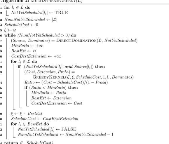
Algorithm 2:MultiStreamGreedy(L) 1 forl_i ∈ Ldo 2 NotYetScheduled[l_i]←TRUE 3 NumNotYetScheduled ← |L| 4 ScheduleCost←0 5 ξ←∅ 6 while (NumNotYetScheduled>0)do

7 (Source,Dominates) = DirectDomination(L,NotYetScheduled) 8 MinRatio←+∞

9 BestExt ←∅

10 CostBestExtension←+∞

11 forl_i ∈ Ldo

12 if (NotYetScheduled[l_i] and Source[l_i])then 13 (Cost,Extension,Proba) =

GreedyKernel(L, ξ,ScheduleCost,1, li,Dominates)

14 Ratio←(Cost−ScheduleCost)/(1−Proba) 15 if (Ratio<MinRatio)then

16 MinRatio←Ratio 17 BestExt ←Extension 18 CostBestExtension←Cost 19 ξ←ξ · BestExt 20 ScheduleCost←CostBestExtension 21 forl_i ∈BestExt do 22 NotYetScheduled[l_i]←FALSE 23 NumNotYetScheduled ←NumNotYetScheduled−1 24 return(ξ, ScheduleCost)

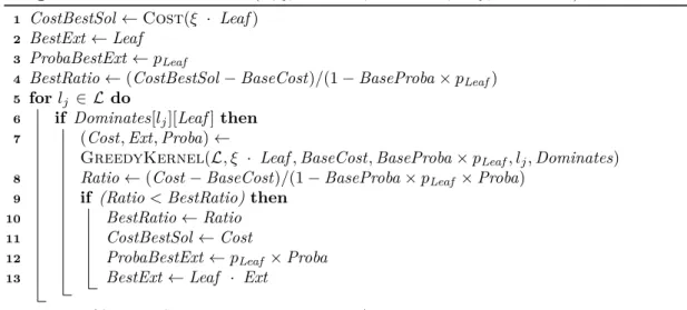
Algorithm 3: GreedyKernel(L, ξ,BaseCost,BaseProba,Leaf,Dominates)

1 CostBestSol←Cost(ξ · Leaf) 2 BestExt←Leaf

3 ProbaBestExt←p_Leaf

4 BestRatio←(CostBestSol−BaseCost)/(1−BaseProba×p_Leaf)

5 forl_j ∈ Ldo

6 if Dominates[l_j][Leaf] then 7 (Cost,Ext,Proba)←

GreedyKernel(L, ξ · Leaf,BaseCost,BaseProba×pLeaf, lj,Dominates)

8 Ratio←(Cost−BaseCost)/(1−BaseProba×p_Leaf ×Proba) 9 if (Ratio<BestRatio)then

10 BestRatio←Ratio 11 CostBestSol←Cost

12 ProbaBestExt←p_Leaf ×Proba 13 BestExt←Leaf · Ext

14 return(CostBestSol, BestExt, ProbaBestExt)

Cost

20000 40000 60000 80000 Shared instances sorted by increasing optimal cost

0 40 80 120 160 0 MultiStreamGreedy Optimal algorithm

Figure 5: Cost achieved byMultiStreamGreedyand that achieved by the optimal algorithm, shown for 81,000 randomANDtree instances sorted by increasing optimal cost.

6

DNF trees

In this section we focus onDNF trees for shared queries. We first show that, as forread-once

queries, there is an optimal schedule that is depth-first (Section 6.1). This result holds in the

multi-streamcase, and thus in the less generalsingle-streamcase. We then show that the problem is NP-complete in thesingle-stream case (Section 6.2), and thus also NP-complete in the more generalmulti-stream case. We then propose and evaluate several heuristics (Section 6.3).

6.1

Dominance of depth-first schedules

Theorem 3. Given a DNF tree, there exists an optimal schedule that is depth-first, i.e., that processesANDnodes one by one.

Proof. Consider aDNF tree T and a schedule ξ. We use the same notations as in Section 4. Without loss of generality we assume that theANDnodes,AND1, . . . ,ANDN, are numbered in

the order of their completion inξ. Thus, according toξ,AND1is the firstANDnode with all its leaves evaluated. We denote byK the number (possibly zero) ofANDnodes that are processed one by one and entirely at the beginning of the query processing according toξ. Therefore, ifξ evaluates a leaf li,j, withi6= 1, in them1 first steps, thenK = 0. Finally, we assume that the leaves of eachANDnode are numbered according to their evaluation order inξ.

We prove the theorem by contradiction. Let us assume that there does not exist an optimal schedule withK=N. Letξbe an optimal schedule that maximizes K. By definition ofK and by the hypothesis on the numbering of theANDnodes, scheduleξevaluates some leaves of the ANDnodes ANDK+2, ..., ANDN before it evaluates the last leaf of ANDK+1. Let ˆL denote the set of these leaves. We now define a new scheduleξ′ _{that starts by executing at leastK+ 1} ANDnodes one by one:

• ξ′ _{starts by evaluating the first K AND nodes one by one, evaluating their leaves in the} same order and at the same steps as inξ;

• ξ′ _{then evaluates all the leaves ofAND}

K+1in the same order as inξ(but not at the same steps);

• ξ′ _{then evaluates the leaves in ˆLin the same order as inξ(but not at the same steps);} • ξ′ _{finally evaluates the remaining leaves in the same order and at the same steps as inξ.} The cost of a schedule is the sum, over all potentially acquired data items, of the cost of acquiring each data item times the probability of acquiring it. Letdbe a data item potentially needed by a leaf inT. We show that the probability of acquiringdis not greater withξ′ _{than withξ. We} have three cases to consider.

Case 1) d is not needed by any leaf ofANDK+1 and not needed by any leaf in ˆL. Thend’s probability to be acquired is the same withξandξ′_.

Case 2) d is needed by at least one leaf of ANDK+1. The only way in which a leaf that is evaluated inξwould not be evaluated inξ′is ifANDK+1 evaluates toTRUE. Since at least one leaf ofANDK+1 usesd, forANDK+1 to evaluate toTRUEdmust be acquired. Consequently, the probability thatdis acquired is the same withξand withξ′_.

Case 3)dis needed by at least one leaf in ˆLbut not needed by any leaf ofANDK+1. ξandξ′ define the same ordering on the leaves in ˆL. For each ANDnodeANDi, withK+ 2≤i≤N,

there is at most one leaf in ANDi∩Lˆ that can be the leaf responsible for the acquisition ofd

withξ, and it is the same leaf withξ′_{. Let F be the set of all these leaves. Then, with ξ, the} leaves inF are responsible for the acquisition ofdif and only if:

• AND1, ...,ANDK all evaluate toFALSE;

• None of the evaluated leaves ofAND1, ...,ANDK needsd; and

Let us denote by P the probability that all the AND nodes AND1, ..., ANDK evaluate to

FALSE and that none of the evaluated leaves of theseANDnodes needs the data itemd. Let us denote by Dthe probability thatdis acquired because of the evaluation of one of the leaves of the ANDnodes AND1, ..., ANDK. Finally, let Rbe the probability that one of the leaves

evaluated withξafterlK+1,mK+1 acquiresd, knowing that no leaves ofAND1, ...,ANDK or in

ˆ

Lacquires it. Then, withξ, the probability pthat dis acquired is:

p=D+P  1− Y li,j∈F 1− j−1 Y k=1 pi,k ! +R (10)

because leafli,j is evaluated with probabilityQjk−=11pi,k, that is, if all the leaves from the same

ANDnode that are evaluated prior to it all evaluate toTRUE. The second term of Equation (10) is the probability that the leaves inF are responsible for acquiringd.

With scheduleξ′_{, the leaves ofF are responsible for the acquisition ofdif and only if:} • TheANDnodesAND1, ...,ANDK, and ANDK+1 all evaluate toFALSE;

• None of the evaluated leaves of theANDnodesAND1, ...,ANDK needd; and

• At least one of the leaves inF is evaluated. Thus, withξ′_{, the probabilityp}′ _{thatdis acquired is:}

p′ _{= D + P 1−} mK+1 Y k=1 pK+1,k ! ×  1− Y li,j∈F 1− j−1 Y k=1 pi,k !  + R.

Comparing this equation with Equation 10, we see thatp′_{is not greater thanp. The probability} that a data item is acquired with ξ′ _{is thus not greater than with ξ. Therefore, in each of the} three cases the cost of ξ′ is not greater than the cost of ξ, meaning that ξ′ is also an optimal schedule. Since ξ′ _{starts by executing at least (K+ 1) AND nodes one by one, we obtain a} contradiction with the maximality assumption onK, which concludes the proof.

6.2

The

single-stream

case is NP-complete

Forread-oncequeries an optimal algorithm forDNFtrees is built on top of the optimal algorithm for ANDtrees in [8]. The same approach cannot be used forshared queries (i.e., reusing Sin-gleStreamGreedy). This can be shown by a simple counter-example (see F). In other words, for some DNF trees, the ordering of the leaves of a given AND node in an optimal schedule does not correspond to the ordering produced by SingleStreamGreedyfor thatANDnode. In fact, we show that finding an optimal schedule for evaluating aDNFtree is NP-complete.

Definition 2 (DNF-Single-Decision). Given asingle-streamDNFtree and a cost boundK, is there a schedule whose expected cost does not exceed K?

Theorem 4. DNF-Single-Decisionis NP-complete.

Proof. The problem is clearly in NP since the expected cost of a schedule can be computed in polynomial time (see Section 4) and compared to K. NP-completeness is obtained via a proof very similar to that of Theorem 2. We build the following instance ofI2 of DNF-Decision:

• We consider a DNF tree with N =n+ 1ANDnodes ANDi, 1≤i≤n+ 1, and a total

ofL= 2n+ 1 leaves.

• The set of streams is S = {A1, . . . , An, B}. The cost of stream si = Ai for i ≤ n is

c(i) = 1