University of Rhode Island University of Rhode Island
DigitalCommons@URI
DigitalCommons@URI
Open Access Master's Theses 2016Network-Based Statistical Methods for the Analysis of Stock
Network-Based Statistical Methods for the Analysis of Stock
Returns
Returns
Zidan WuUniversity of Rhode Island, [email protected]
Follow this and additional works at: https://digitalcommons.uri.edu/theses
Recommended Citation Recommended Citation
Wu, Zidan, "Network-Based Statistical Methods for the Analysis of Stock Returns" (2016). Open Access Master's Theses. Paper 948.
https://digitalcommons.uri.edu/theses/948
This Thesis is brought to you for free and open access by DigitalCommons@URI. It has been accepted for inclusion in Open Access Master's Theses by an authorized administrator of DigitalCommons@URI. For more information, please contact [email protected].
NETWORK-BASED STATISTICAL METHODS FOR THE ANALYSIS OF STOCK RETURNS
BY ZIDAN WU
A THESIS SUBMITTED IN PARTIAL FULFILLMENT OF THE REQUIREMENTS FOR THE DEGREE OF
MASTER OF SCIENCE IN
STATISTICS
UNIVERSITY OF RHODE ISLAND 2016
MASTER OF SCIENCE THESIS OF
ZIDAN WU
APPROVED:
Thesis Committee:
Major Professor Natallia Katenka Gavino Puggioni Correy Lang
Nasser H. Zawia
DEAN OF THE GRADUATE SCHOOL
UNIVERSITY OF RHODE ISLAND 2016
ABSTRACT
To maximize returns and diversify a financial portfolio, the stock price market participants have always been interested in learning associations of stock price returns for different companies. Five primary goals of this thesis are: (1) to evaluate and infer associations of stock returns between different companies in selected industrial sectors and countries, and (2) to identify groups of companies that exhibit the most similar stock market trends, and (3) to evaluate changes in associations between companies in time period from 2009 to 2015, (4) to forecast future return movements using selected classification methods, and (5) to explore the relationship between the accuracy of classification of stock return movements and network node properties.
This thesis analyzed daily stock price data collected from publicly available sources, Yahoo Finance, for a sample of eighty-nine selected companies from four industrial sectors and three countries (China, Germany, and the US) for a time period of seven years from 2009 to 2015. Daily prices were converted into returns and then used to compute a correlation matrix and a corresponding association network. Obtained network was employed to identify clusters of companies that exhibit similar return trends and to evaluate the relationships within and between different industrial sectors. To assess changes in associations between companies during special financial events, annually dynamic networks were created. Four classification methods, namely Linear Discriminant Analysis, Quadratic Discriminant Analysis, k-Nearest Neighbors, and Logistic Regression were built to predict price movements for all selected
companies. The relationships between classification accuracy rates and network properties were evaluated graphically.
The results of the network-based analysis showed that the companies that traded in the same stock market and/or belonged to the same industrial sector had significant associations. Specifically, Chinese companies had higher inner correlations in banking and telecommunication sectors; the US and German companies had stronger associations in banking and auto manufacturing sectors. Interestingly, the associations among companies became stronger and more companies tended to be grouped together in the network during significant financial events and in the early recovery periods. The results of classification analysis revealed the superior performance of logistic regression method compared to other three classification methods, particularly for the Chinese companies. Remarkably, companies that acted as followers and belonged to medium-size clusters with eight to thirteen neighbors in the association network were easier to classify than other companies, thereby supporting the relationship between classification and network-based methods.
Keywords:
Association network, stock price return, hierarchical clustering, logistic regression, classification, forecasting.
iv
ACKNOWLEDGMENTS
It is my great pleasure to thank the numerous people who help and support me during my two-year study in University of Rhode Island. Their constant help and support make my two-year study extremely fascinating and memorable.
Firstly, I would like to give the deepest thanks to my advisor Natallia Katenka for her inspiration, advisory and supervision throughout my entire graduate study. Her unconditional support through all aspects in the research and non-research world. She
devotes countless hours of her personal time to help me finish my research and thesis; her valuable advice helps me get a wonderful intern opportunity and a job offer; and her scrupulous spirit and keeping on improving attitude deeply affects me and will continuous impresses me in my future career and life.
I also would like to express my appreciation to my committee members Professor Gavino Puggioni, Professor Corey Lang. Their considerable professional knowledge and experience supports me both through courses in the Statistics and through research. My thanks also go to Professor Xiaowei Xu.for her great help and patience as the chair of the committee.
Through the past two years of my study, I am greatly supported by Professor Liliana Gonzalez, the head of Statistics, who gives me all kinds of invaluable academic advices and guidance. She also gives me the opportunity to work as a teaching assistant during the two-year study in Statistics program.
Last but not the lease, I would like to express my appreciation to my husband, Yao Lu, for his love, patience, and support throughout the completion of this thesis. I
v
am also truly in debt on my parents for their love, encouragement and support. Without their support, I would never be able to pursue my dream at University of Rhode Island.
vi
TABLE OF CONTENTS
ABSTRACT ... ii
ACKNOWLEDGMENTS ... iv
TABLE OF CONTENTS ... vi
LIST OF TABLES ... viii
LIST OF FIGURES ... ix
CHAPTER 1 INTRODUCTION ... 1
CHAPTER 2 REVIEW OF LITERATURE ... 6
CHAPTER 3 DATA DESCRIPTION AND PREMINARY ANALYSIS ... 10
3.1 Data Collection ... 10
3.2 Data Preparation ... 13
3.3 Preliminary Analysis ... 15
3.3.1 Returns ... 17
3.3.2 Return Distribution ... 17
3.3.3 Stock Return Correlation and Annual Volatility ... 20
CHAPTER 4 METHODOLOGY ... 26
4.1 Correlation-Based Network ... 27
4.1.1 Threshold Correlation Network ... 29
4.1.2 Random Graph Models ... 30
4.1.3 Network Characteristics ... 31
4.2 Network Community Detection ... 34
4.3 Dynamitic Networks ... 37
4.4 Classification Methods ... 38
4.4.1 Linear Discriminant Analysis ... 39
4.4.2 Quadratic discriminant analysis ... 40
4.4.3 K Nearest Neighbors ... 42
vii
4.5 Evaluation of Model Performance ... 44
CHAPTER 5 RESEARCH RESULTS ... 46
5.1Correlation-Based Network ... 46
5.1.1 Threshold Network ... 48
•Threshold Value Selection ... 48
•Characteristics of the threshold Network ... 51
•Assessing Significance of Network Characteristics ... 52
5.1.2 Visualization of Network ... 55
5.2 Network Community detection ... 56
•Reduced Network ... 59
5.3 Dynamitic Analysis Result ... 59
5.4 The Performance of Four Classification Models ... 62
5.5 Associations Between Network Features and Regression Model Performance ... 67
CHAPTER 6 CONCLUSION ... 71
BIBLIOGRAPHY ... 73
viii
LIST OF TABLES
TABLE PAGE
Table 1 Companies distribution within 3 countries and 4 industries. ... 11
Table 2 Summary of returns for three countries and across 7 years. ... 19
Table 3 Mean correlation across 3 countries and 4 industries. ... 22
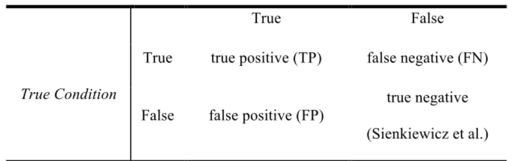
Table 4 The confusion table layout ... 45
Table 5 Significance test results of Network characteristics ... 54
Table 6 Table of Network Characteristics across 7 research years from 2009 to 2015. ... 60
Table 7 The prediction accuracy of LDA model across 3 different countries ... 64
Table 8 The prediction accuracy of QDA model across 3 different countries ... 64
Table 9 The prediction accuracy of KNN model across 3 different countries. ... 65
Table 10 The prediction accuracy of Logistic regression model across different countries ... 65
ix
LIST OF FIGURES
FIGURE PAGE
Figure 1 The stock market index performance and linear trends for three countries ... 2
Figure 2. The price chart over 7 years for stock prices of three selected banks ... 16
Figure 3 Average returns as a function of time. ... 18
Figure 4 Chi-square plot of generalised distances for the returns ... 20
Figure 5 Correlations matrix and histogram of correlation coefficients.. ... 21
Figure 6 Left panel: annual average correlation (plotted in red) and average volatility (plotted in blue) as a function of time. Right panel: annual average volatility as a function of time for three different countries. ... 24
Figure 7 Left panel: Network graph with all potential edges. Right panel: Correlation network has significant edges only. ... 48
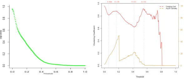
Figure 8 Network Characteristics as functions of different correlation threshold values ... 50
Figure 9 Threshold Network graphs inferred from different correlation thresholds. ... 51
Figure 10 The distributions of different Network Characteristics ... 52
Figure 11 The distribution of classical random graphs’ characteristics ... 53
Figure 12 The distribution of generalized random graphs’ characteristics ... 53
x
Figure 14 Hierarchical clustering dendrogram ... 59
Figure 15 The reduced network graphs ... 59
Figure 16 Annually Dynamic Network in the time period from 2009 to 2017 ... 62
Figure 17 The predictive performance of 4 classification models ... 66
Figure 18 The scatter plots between classification accuracy rates and threshold network node properties. ... 68
Figure 19 The level plots of the relationship between classification accuracy rate and network node properties ... 69
1
CHAPTER 1 INTRODUCTION
INTRODUCTION
A stock market is also known as an equity market, which is the market issuing and trading shares of publicly held companies. A stock market is comprised of buyers and sellers of stocks, or shares, of different companies. The main function of any stock market is to allow companies to trade their stocks and raise additional financial resources for future growth and development. The stock buyer and seller could be institutes or individuals. Naturally, maximization of the selling price and minimization of the buying price are the main aims of seller and buyer. The appeal of the stock market is strong. According to the WilmerHale 2016 IPO (Initial Public Offering) report (WilmerHale 2016), 963 companies have entered the US stock market and started to sell their companies’ shares from 2009 to 2015.
Besides the befit to companies and investors, the stock market serves as a primary indicator of economic stability. The stock prices of leading companies evaluate the state of development and economy of different countries and/or industries. For example, the Standard and Poor's 500 (S&P500) index that is constructed by 500 large companies selected based on their market capitalization and common shares listed for trading on the NYSE or NASDAQ. Therefore, the S&P 500 is known as one of the most internationally recognized equity indices, and it is also considered to be one of the best of representations of the US Economy. Similarly, the Shanghai Composite Index (SHCSI) shows the Chinese companies performance in Shanghai Stock Exchange. Deutsche Aktienindex (DAX) known as a German stock index is
2
constructed by 30 major German companies traded on Frankfurt Stock Exchange. Unlike American S&P 500 indexes, DAX index is measured by the performance of only 30 largest German companies. Due to the small sample size selection, DAX couldn’t well present the vitality of the Germany economy.
The performance of three indices, S&P500, SHCSI and DAX, from 2009 to 2015 is given in Figure 1, which shows an increasing trend for all selected countries. The slopes of the German and the US indices are significantly sharper compared to the Chinese index indicating these two countries’ economy are bouncing back and gradually exiting the recession. The Chinese index is not stable since there is a sharply increasing trend from second quarter of 2014 to first quarter of 2015. The German and the US indices have similar trend patterns from January of 2009 to the end of second quarter of 2014. The Chinese index and German indices have similar trends from the second quarter of 2014 to the end of 2015. Generally, the stock market is a complex index that is influenced by performance of a subset of large companies. Analysis of associations between indices can only help to find the associations between different countries, but not specific companies.
0 2000 4000 6000 8000 10000 12000 14000 0 1000 2000 3000 4000 5000 6000 2009 2010 2011 2012 2013 2014 2015 US Chinese German Linear (US) Linear (Chinese) Linear (German)
3
Beyond discovering associations between financial indices of different countries, recovering the associations between companies based on their stock price returns is a complicated, but an important task that has received much interest among investors and financial researchers. The pair trading used in financial corporations and hedge fund is a very illustrative example of utilizing the association between different companies to gain profits.
The pair trading has been originally proposed by Gerry Bamberger and Nunzio Tartaglia’s quantitative group at Morgan Stanley (Bookstaber 2007). Pair trading is done by closely monitoring two stocks whose prices are highly correlated. When the two stocks temporarily go out of sync, the trader would long the stock that is relatively lower in price and short the one that is higher in price. This way when the two stock prices converge again, the trader would benefit from his long and short positions.
The simultaneous long and short selling are widely used trading techniques in pair trading that aim at gaining profits from the relative movement of stock prices in both an upward trend market and a downward market (Ehrman 2006). For instance, consider one classic pair of companies, Coca Cola and Pepsi, two companies that produce a very similar soda product and have highly correlated stock prices. Historically, the stock prices of Coca Cola and Pepsi have had similar stock digs and highs depending on the soda market. It is expected that their price return movements to be same. However, sometimes the associations of these two companies are not synchronic. For example, the Coca Cola stock went up a significant amount while Pepsi stayed the same. Traders would buy the stocks of the long underperforming Pepsi and sell or short the stocks of the outperforming Coca. They would bet buying
4
Pepsi at a lower price, while selling Coca at a high price, assuming that these two companies would latter return to their historical balance. The benefit could be realized if the Pepsi stock price goes up or the Coca Cola price goes down. Wal-Mart and Target is another example of companies that sell very similar products and where pair trading could be used effectively. Thus, inferring and analyzing associations of stock returns between different companies may prove to be useful for financial researchers in both academic and corporate worlds. Additionally, it would be valuable to create reliable predictive models of price return movements and evaluate the relationships between this models and inferred associations.
Five primary goals of this thesis include: (1) evaluation and inference of associations of stock returns between different companies in selected industrial sectors and countries using correlation networks, and (2) identification of the groups of companies that exhibit the most similar stock market trends using network-based community detection techniques, (3) evaluation of dynamic changes in associations between companies in time period from 2009 to 2015 using dynamic networks, (4) forecast of future return movements using parametric and non-parametric classification methods, and (5) assessment of relationships between the accuracy of classification of stock return movements and network node properties.
To achieve these goals, daily historical stock price data was collected from publicly available national and international sources for multiple companies in selected industrial sectors in the US, China, and Germany for a period of seven years (from 2009 to 2015). Obtained prices were utilized to create a correlation matrix and characterize corresponding association network. The network properties, such as the
5
average node degree, network density, clustering coefficient, and average betweenness centrality, were computed for the generated correlation network. The network-based community detection method was used to find the cohesive sets of companies that exhibit the most similar stock return trends. Note that outlined network characteristics and community detection were applied to stationary network (inferred from all seven years of data) and a sequence of dynamic networks (inferred from annual data). The purpose of analysis of dynamic (annual) networks is to assess changes in associations between companies during special financial events. Since many companies depend on loans and credits, fluctuations in their stock prices may affect the stock prices of their lenders in other industries. As a result, the associations between different companies could change over time especially when facing big financial event and in the periods of early market recovery. To predict future stock return trends, parametric classification methods, including linear discriminant analysis (LDA), quadratic discriminant analysis (QDA), and logistic regression, and non-parametric k-nearest neighbor method, were applied to collected price data.
The rest of this thesis is organized as follows. Chapter 2 reviews related work in network-based and multivariate analysis of financial data. Chapter 3 outlines the data collection process and preliminary data analysis. Chapter 4 describes the network methods and predicting models used in this thesis. Results and Conclusion are summarized in Chapter 5 and Chapter 6.
6
CHAPTER 2 REVIEW OF LITERATURE
REVIEW OF LITERATURE
Application of correlation networks to the analysis of associations between different companies and/or countries based on stock market prices or exchange indices has received considerable attention among statisticians and financiers over the last ten years (Heimo et al. 2007; Nobi et al. 2014; Sienkiewicz et al. 2013; Song et al. 2011).
To analyze the association movement in stock market data, correlation graphs are often used to infer associations among the countries, industries, and/or companies, and then more sophisticated network-based techniques are employed to extract information about the global structure of the stock market. For example, correlation graph-based approach has been used to analyze the presence of both short-term and long-term association dynamic among stock exchange indices of 57 countries in the time period from 1996 to 2009 by Song (Song et al. 2011). Threshold-based correlation networks have been utilized to explore the effect of global financial crisis of 2008 on the association of stock prices in local Korean stock markets by Nobi (Nobi et al. 2014). stock returns of 96 US companies from 2005 to 2012 have been used to build a correlation network and analyze the movement of both credit and stock market during and after 2008 financial crisis by Lim (Lim et al. 2014). The maximal spanning tree of 116 US stocks returns (collected in the period from 1997 to 2000) has been constructed based on the correlation network, and then used for identification of the industry sectors of central nodes in the network by Heimo (Heimo et al. 2007).
7
Besides analyzing the association movement in stock market data, using historical data to create an optimal predictive model for current and future events became very popular in the new millennia (Leung, Daouk, and Chen 2000; Wang and Shang 2014; Kara, Acar Boyacioglu, and Baykan 2011; Alrasheedi 2012; Nguyen, Shirai, and Velcin 2015; Zhang et al. 2015; Peng 2015).
Specifically, to predict the movement direction of future stock price/index, many various statistical and machine learning classification models, such as Linear Discriminate Analysis (LDA), Artificial Neural Network (ANN), Support Vector Machines (SVM), have been applied to financial data. For example, the relationship between historic records of three indices, SP500, FTSE, Nikkei, and short term interest rate data in the period from 1967 to 1995 have been utilized to build models and test the predictive strength of constructed classification models via LDA, Logit and Probit Logistic Regression (Leung, Daouk, and Chen 2000). Wang and Shang converted the historic close price, high price and low price into different predictors, and applied the Lease Squares Support Vector Machine to forecast the direction of Chinese Security Index 300, as well, the LDA, QDA and Neural Network served as comparing model (Wang and Shang 2014). Kara and Boyacioglu used the the ANN and SVM model to predict the movement direction of daily Istanbul Stock Exchange National Index 100 (Kara, Acar Boyacioglu, and Baykan 2011).
Most of the projects listed above rely on historical data of only one type (e.g., prices, returns, etc.). More recently, other sources of information have been used to build models with better performance. For instance, to predict the stock price direction of one large industry corporation in Saudi Arabia, the authors have used the historical
8
price data, volume data, crude oil price and indices, Dow Jones and Saudi Index (Alrasheedi 2012). The sentiments from social media have been used to build a predictive model for stock price movements by Nguyen et al. (Nguyen, Shirai, and Velcin 2015). Recently, Zhang and Li have proposed a new stock movement predictive model that has shown a superior performance of energy sector. Proposed model incorporated market capitalization of multiple companies and sentiments from Twitter associated with these companies (Zhang et al. 2015). Similarly, financial data collected from Bloomberg has been used as an additional predictor for a neural network model forecasting stock price movement (Peng 2015).
To predict the future stock price return or volatility, many time series models, such as Autoregressive (AR), Autoregressive Integrated Moving Average (ARIMA) and Generalized Autoregressive Conditional Heteroscedasticity (GARCH), have been proposed. The time series model normally uses the previously observed values to predict the future output. For instance, the output of autoregressive model at time t is a linear regression of its own previous values. The AR(2) model uses previous two-day records, that is the value at time t-1 and the value at time t-2, as predictor-one and predictor-two to forecast the output at time t. In this study, instead of using the time series notion to build the optimal predictive model, the focus is on comparing the predictive performance of different objects by using the same predictors.
Unlike previous research that focused on exploring the changes of association of global and local exchange indices, the research in this thesis focuses on evaluating association among a subset of leading companies that comprised multiple industries (banking, communication, manufacturing, and pharmaceutical) in three countries with
9
high market activity (USA, Germany, and China) located on three different continents (North America, Europe and Asia). Additionally, the correlation based threshold network is used to detect and clearly represent the associations between companies and to discover the clusters of companies following the most similar trends. Besides the static network, the annual dynamic network is employed to assess changes in associations between companies in the time period from 2009 to 2015. Also, four classification models are created and compare the prediction performance of different objects across 3 different countries under the same treatment and standard. The six years’ historical data in the period from 2009 to 2014 are utilized as predictors to create the classification models, and the accuracy rate is used as a justification to evaluate the performance of different models. Finally, to find the relationships between classification accuracy rates and network node properties, graphical tools are applied here to evaluate the relationship, such as the scatter chart and level plot.
10
CHAPTER 3 DATA DESCRIPTION AND PREMINARY ANALYSIS
DATA DESCRIPTION AND PRELIMINARY ANALYSIS
In order to perform a robust and an accurate data analysis that would bring valid insights, it was essential to go through three data processing steps: data collection, cleaning, and formatting. Section 3.1 explains how the data was initially obtained from a large financial data source provider, Yahoo Finance. Section 3.2. Illustrates an extensive data cleaning process that was applied to improve the data quality. Specifically, Section 3.2 focuses on situations with missing data values or differences in trading dates. Additionally, this section describes how all collected stock prices were converted to the US dollars to ensure the stock returns to be comparable across different companies, industry sectors, and countries. Finally, Section 3.3 provides the results of an extensive preliminary analysis in order to understand the data and to present a reader with a general overview of the data.
3.1 Data Collection
Public daily closing stock prices recorded between Jan 2nd 2009 to Dec 31st 2015 were collected from Yahoo Finance for a subset of leading companies from multiple industrial sectors (banking, communication, manufacturing, and pharmaceutical) in three countries with high market activity (USA, Germany, and China). Closing prices were chosen as a proxy for the most accurate and commonly used measures of stock price values when financial data was collected on a daily basis.
11
The distribution of the companies among four industries in three countries is as follows in Table 1.
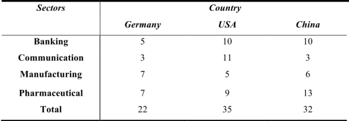
Table 1 Companies distribution within 3 countries and 4 industries.
Table 1 shows that the number of leading companies in communication sector in Germany and China is much smaller than the number of the US communication companies. The US telecommunication market is a liberalization market and it was subdivided into 3 main classes: one class is the large integrated telecom companies, such as AT&T, Verizon and Sprint, providing both wireless and wireline service; second class is the large wireless companies, such as T-Mobile, and the third class is the regional wireline companies, such as Frontier, CenturyLink, etcetera. However, the Chinese telecommunication system is different from the US system, it was divided by 3 companies that the Chinese government possesses. The number of leading US Auto-manufacturer is small due to the high concentration of auto market, where the head 5 manufacturers produce over 13 auto brands and occupy over 35% of the US auto-sale market.
The total of 35 US companies, 22 German companies, and 32 Chinese companies was selected as the dataset for this research. The complete list of company names, countries, and stock symbols is recorded in Appendix A.
Sectors Country
Germany USA China
Banking 5 10 10
Communication 3 11 3
Manufacturing 7 5 6
Pharmaceutical 7 9 13
12
In this study, all selected US companies are trading in the largest stock exchange: New York Stock Exchange (NYSE) and using the US Dollars as their trading currency; all selected German companies are trading in Frankfurt Stock Exchange (FSE) market in Frankfurt and they are using Euro as their trading currency; thirty selected Chinese companies are trading stocks in Chinese local stock market, Shanghai Stock Exchange (SSE), using CNY as their trading currency, and three Chinese communication companies, China Mobile Ltd, China Unicom and China Telecom Corporation, are trading their company shares in NYSE as American depositary receipt (ADR) using US Dollars as their exchange currency. It is worth noting that ADR is a stock that is traded in the US but represents a certain number of shares for a foreign stock.
Analyzing stock prices in different currencies can cause potential problems since the currency exchange rates are floating rates and can change rapidly. If the currency rates diverge greatly in a certain period of time, the analysis of the stock prices would be thus inaccurate for foreign stocks. This will compromise our ability to extract clean financial time series from the stock prices. In order to eliminate differences in currencies of obtained stock prices and to explore the associations between companies, all stock price currencies were converted to the US Dollars. The daily currency exchange rates were collected from Oanda Corporation, a Canadian foreign currency exchange company, for a period of time between 2009 and 2015. After converting all currencies to the US Dollars, the datasets for all three countries were stored in the same units, the US Dollars.
13 3.2 Data Preparation
The project data was collected in a period time from Jan 2nd 2009 to Dec 31st 2015; however, the date when the companies were listed on the public stock market varies. Not all selected companies started trading before 2009; some companies remained private before 2009 and started trading their company shares publicly after 2009. e.g., Tesla Motors in the US, Agriculture Bank in China, and Telefónica in Germany. As a result, there are multiple missing stock price records that could potentially complicate the analysis in this project. If a company started trading after Jan 2nd 2009, the records from Jan 2nd 2009 till the first business day before the Initial Public Offering (IPO) date would be unavailable. The records during that period are absent. Before doing further analysis, missing value imputation method was employed to the data. The numeric value of one was filled in the missing value position for the following reasons.
First reason is that since the stock returns were used for further analysis in this research, feeling zeros instead of ones in the missing records positions would result in non-identifiable values of log of zero. Clearly, such values should be avoided, for example, when computing correlations and performing classification analysis.
Second reason is that one needs to keep sufficient historical information available from the data for further data analysis. For instance, three companies did not have part of the stock price records due to IPO reason. If one completely gets rid of companies (variables) with missing values, it may cause some sectors having significantly fewer companies compared to other industrial sectors, thereby making analysis of this sector less interesting and less reliable. For example, the number of automobile
14
manufacturing companies in the US is already small. Tesla, a new revolutionary car manufacturer leveraging new environmental friendly electronic energy instead of gasoline, did not start trading until June 2010, but expanded its market share rapidly in the last few years. There will be significantly fewer companies in selected sectors if one removes companies like Tesla from the dataset. Computationally, it is also more convenient merging different datasets without missing values. Note that to fill in missing values after company IPOs, imputation regression method was employed.
One more data issue is related to duplicated records. Stock market stops trading on holidays and different countries have their own national holidays. For example, the NYSE market is closed on President's Day and Good Friday in the US, and Shanghai Stock Exchange (SSE) market is closed for 7 days during Guoqing Festival. In the US, if the market is closed a day, it keeps no record for that day. However, Chinese market keeps the previously available record as holiday trading record in Yahoo finance. For example, during Chinese Guoqing Festival from October 1st, 2015 to October 7th, 2015, the Shanghai stock exchange market was closed, but the Yahoo finance still kept stock records from a day before holidays (September 30th 2015) and used it as real stock records for the next 7 days. Thus, the record of September 30th 2015 was used 8 times. Realistically, the records during holidays cannot be considered historical records. In order to keep more realistic data records, duplicated records in the research data were removed (e.g., 7 days from October 1st 2015 to October 7th 2015).
After removing duplicated records and solving missing values, the total of 1640 trading day was recorded for Chinese companies, 1778 days and 1761 days for German and the US companies, respectively. Combining data for all three countries
15
and keeping only common trading day records resulted in 1621 common trading days to be used in this research.In what follows, we present a general overview of the data to the reader. And we organized the rest of the chapter as follows: in Section 3.3.1 we describe how we use method to normalize research data and reduce the variance of the stock changes; in Section 3.3.2 we discuss the distribution of return varies for 3 countries across 7 years; in Section 3.3.3 we use Pearson correlation to analyze the create the correlation matrix and evaluate how the average relationship and volatility varies as a function of time.
3.3 Preliminary Analysis
Price chart and Candlestick Chart are commonly used plots for financial representation that are used to describe how a stock evolved over a given period of time. The following three price charts depicted in Figure 2 show how the closing prices of Post Bank, Citi Bank and ICBC changed over 7 years from the beginning of 2009 till the end of 2015.
16
Figure 2. The price chart over 7 years for stock prices of three selected banks: Post Bank, Citi Bank and ICBC trading in Germany, the US, and China, respectively)
Figure 2 represents Post Bank having an unsatisfied continuously decreasing trend after 2010. Its stock price decreased 66% from January 2010 to December 2015. The Citi Bank had a severe depression around 2012 and a rapid recovery after 2012; and the stock prices of ICBC change in a limited range following a similar pattern of movement as Chinese stock index.
The reasons of causing stock rise or fall vary. In generally, there are three main factors that could affect stock price movements. First factor is a fundamental performance of a company, for example, the change of management, the earnings and profits related news, release of a new product, lay-off employees and etc. Second
17
factor is related to the industry performance and behavior of competitors. The last factor is related to the overall national economy and economic policy.
3.3.1 Returns
In this thesis, the returns were calculated and would be applied for the further analysis. Compared to stock prices, the big benefit of using stock returns instead of stock price is that the stock returns reduce the variance of stock changes, or volatility. Apparently, the stock price would have extremely large change compared to the previously recorded price especially during significant financial events. Song et al. (D.-M.Song, 2011) explored this phenomenon for several financial events including the 1997 Asian crisis, 1998 Russian Crisis and 2008 global crisis. The daily return is computed by the following equation:
!" # = ln '" # - ln '" #-1 , [1]
where is the closing price of company i on day t. 3.3.2 Return Distribution
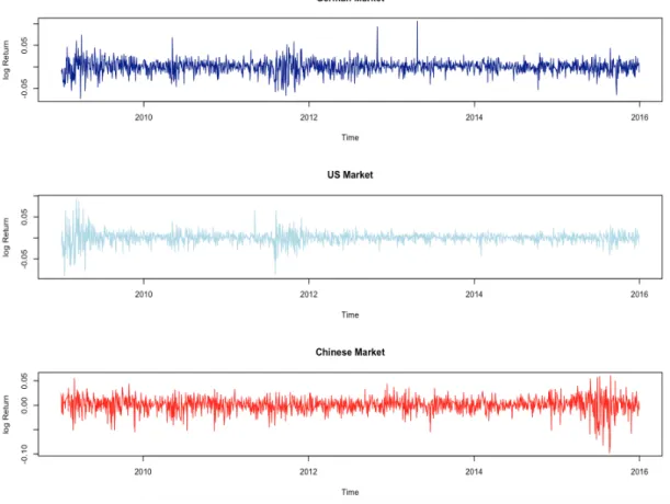
Eighty-nine companies were selected for this project, where each country had 20 to 30 companies. In what follows in Figure 3, the averaged returns are represented as a function of time for each country; the X-axis represent a seven-year timeline from 2009 to 2015 and the Y-axis stands for the corresponding stock returns records.
18
Figure 3 Average returns as a function of time. The X-axis represents 7-years timeline from 2009 to 2015; the Y-axis stands for the corresponding stock returns
records.
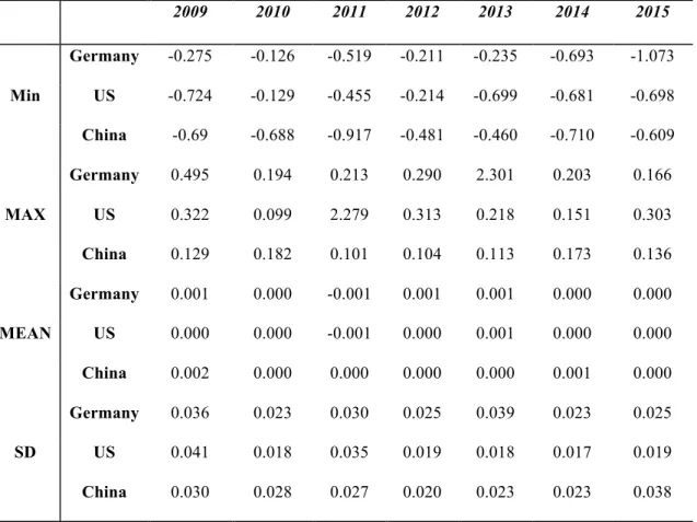
Figure 3 shows that the three distributions of daily average returns have mean zero and. Daily stock returns change in a small range from negative 0.05 to positive 0.05. This illustrates how stock returns would normally change upward or downward in less than 5% compared to yesterday returns. Figure 3 also shows that there are three significant fluctuations around 2009, 2011 and 2015 of different intensities for different countries. This suggests that Germany, the US and China have different state effects caused by a global financial crisis in 2008. During following 2-3 years of the financial recession period, world economic market presents a declining trend, but the exact time of the recession varies from country to country. Another significant
19
fluctuation can be observed in 2015. In the third and fourth quarters of 2015, Chinese financial stock market, a second economy market in the world, crashed. This led to visible market fluctuations in the Western Europe stock market. There are multiple reasons causing Chinese stock market to crush including slowing down industry, the devaluation of Chinese currency, and the government froth cleaning strategy, to name a few. 2009 2010 2011 2012 2013 2014 2015 Min Germany -0.275 -0.126 -0.519 -0.211 -0.235 -0.693 -1.073 US -0.724 -0.129 -0.455 -0.214 -0.699 -0.681 -0.698 China -0.69 -0.688 -0.917 -0.481 -0.460 -0.710 -0.609 MAX Germany 0.495 0.194 0.213 0.290 2.301 0.203 0.166 US 0.322 0.099 2.279 0.313 0.218 0.151 0.303 China 0.129 0.182 0.101 0.104 0.113 0.173 0.136 MEAN Germany 0.001 0.000 -0.001 0.001 0.001 0.000 0.000 US 0.000 0.000 -0.001 0.000 0.001 0.000 0.000 China 0.002 0.000 0.000 0.000 0.000 0.001 0.000 SD Germany 0.036 0.023 0.030 0.025 0.039 0.023 0.025 US 0.041 0.018 0.035 0.019 0.018 0.017 0.019 China 0.030 0.028 0.027 0.020 0.023 0.023 0.038
20
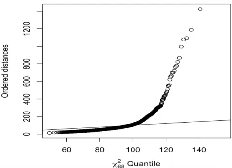
Figure 4 Chi-square plot of generalised distances for the returns
In order to preliminarily observer and visual check the normality of the returns, the Chi-square Q-Q plot is created, where X-axis is the expected distance and Y-axis is the actual distance. If returns follow a multivariate normal distribution, the points on the graph should approximately lie on a straight line, otherwise, the points are off the line. The Figure 4 represents numerous points are skewed and not on the line. Thus, one cannot infer the research data follow a normal distribution.
3.3.3 Stock Return Correlation and Annual Volatility • Pearson Correlation Matrix
Pearson correlation is one of the most popular statistical measures that evaluates an association between two different numerical sets. Pearson correlation can be used to estimate the similarity between stock returns of two companies i and j as follows:
ρ"# =
σ"#
21
where {σ"#} is a sample covariance between stock returns of company i and
company j, and
σ
"", σjj are the sample variances of stock returns of company i and company j, respectively. Figure 5 illustrates estimated values of the correlation coefficientρ
"# between companies i and j obtained from 7 years of daily collected data. Naturally, a correlation coefficient ranges from -1 to 1 with higher positive values indicating direct linear relationship between stock returns.
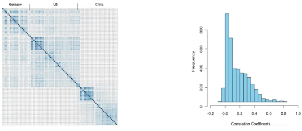
Figure 5 Correlations matrix and histogram of correlation coefficients. In the correlation matix figure (left panel), the darket color indicates stronger correlation
between companies. Two figures were created using the entire 7-year period.
The summary of correlation coefficients computed from daily stock returns between different companies is illustrated in Figure 5. The left panel of Figure 5 illustrates a correlation matrix that demonstrates that the majority of correlation values are positive meaning the most companies returns followed same trends. The right panel of Figure 5 supports this conclusion that is the distribution of correlation coefficients is right-skewed with values ranging from -0.1 to 0.85.
22
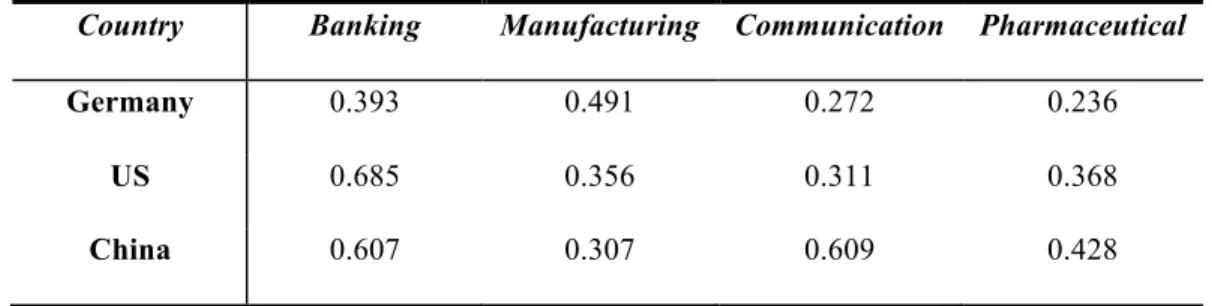
Country Banking Manufacturing Communication Pharmaceutical
Germany 0.393 0.491 0.272 0.236
US 0.685 0.356 0.311 0.368
China 0.607 0.307 0.609 0.428
Table 3 Mean correlation across 3 countries and 4 industries.
In order to evaluate the inner correlation across 3 countries and 4 industries, we computed the average correlation coefficients and summarized the results in Table 3. One can see that the inner correlation of German Communication and Pharmaceutical is smaller than other two German sectors, especially the German Manufacturing. US banking has the largest inner correlation which equals to 0.685. As well, the Chinese communication and banking has greater inner correlation than the other two Chinese industries.
• Returns Annual Volatility
Volatility is also known as the variation of a stock or index, and it could estimate how risky a particular stock/ index is (Ensor,2014). Volatility could be measured using the security’s standard deviation, which describes how tightly the stock prices are distributed around the mean. Because the value of standard deviation is always positive, volatility is also positive. In this section, the annual average volatility is measured as follows:
!"##$%& = !() * , , [3]
where !"# is the standard deviation of a daily return, and P is the time period of return.
23
Left panel of Figure 6 plots the annual average correlation and volatility 89 companies under consideration. The annual average correlation shows an upward trend before 2011 reaching its peak in 2011 with value of 0.26. The rapid increase in trend can be explained due to the European sovereign debt crisis in some European countries. This financial crisis could cause an 18% increase in the average correlation. After 2011, the average correlation decreased by 50% from 2012 to 2014 and sharply increased by 61% from 2014 to 2015, which can be attributed to Chinese financial crisis.
It is well known that high volatility in stock market is related to special financial events (S. Leonidas,2012). In general, the correlation would change with volatility. In the left panel of Figure 5, one can see that the mean correlation and the average volatility have same movement trend between 2010 and 2015. During special financial events, such as European debt crisis in 2011 and Chinese stock market turbulence in 2015, the average volatility increased to 15% and 18%, respectively.
24
Figure 6 Left panel: annual average correlation (plotted in red) and average volatility (plotted in blue) as a function of time. Right panel: annual average volatility as a
function of time for three different countries.
The right panel of Figure 6 demonstrates the annual average of historical return volatility for all selected companies in Germany, the US and China combined. This graph shows that the US and Germany volatility have same downward trend with two lines to be approximately parallel. The volatility of Germany changes to 31% in the time period from 2009 to 2015, whereas the mean volatility of US changed to 36% in the same period. The volatility of the US stock returns is greater than the volatility of German stock returns a year after the global financial crisis in 2008. In 2009, the volatility of the US returns has the largest hit compared to China and Germany. In this period the majority of the US companies relived dramatic changes. In 2009, many American companies started their recovery while others were still in recession which could explain relatively high volatility in 2009. A sharp increase in the volatility (up to 67% in one year) was also observed in 2015 in China that could be attributed to Chinese stock market turbulence. Other financial events could also contribute to significant changes in the average correlation and the average volatility, but they remained beyond the scope of this project.
The findings of the preliminary analysis present that the return has a mean zero and varies in a small range. The majority positive correlation coefficients between different companies implied that most companies’ returns followed same trends and were affected by the national economy. The volatility represented the variation of returns and usually has a similar trend with the average correlation of 89 research companies. However, the volatility only refers the variation of a specific asset or index
25
and can not provide information on how the relationship changes within the research data. Thus, in order to fill the gap and detect the associations between companies, we will introduce and describe the network-based analysis methods and classification models in the following chapter. The main findings and conclusion of proposed study are summarized in Chapter 5 and Chapter 6.
26
CHAPTER 4 METHODOLOGY
METHODOLOGY
The methodology used in this thesis mainly focuses on two important domains of statistical analysis. The first domain, statistical analysis of network data, is used to evaluate the relationships between selected companies based on their daily stock returns and to infer and characterize association networks. The second domain, classification analysis, is aimed at forecasting the direction of future returns of stocks using classification techniques such as linear discriminant analysis (LDA), quadratic discriminant analysis, logistic regression and a non-parametric model, k-nearest neighbors (KNN).
Specifically, Section 4.1 introduces how the association networks are built utilizing correlations computed between time series of stock return of different companies, and illustrate the principles of FDR test which aims at avoiding generating exaggerated type I error. Section 4.2 focuses on the threshold network model which is adapted to explain large and complex networks. In addition, Section 4.3 and Section 4.4 describe methods for computing network characteristics and the process of testing the significance of the computed characteristics. Section 4.5 further clarifies how the annual networks were inferred in this research. Finally, Section 4.5 focuses on the four classification methods that are used for forecasting the direction of future stock returns.
27 4.1 Correlation-Based Network
Statistical analysis of network data combines an area of mathematical graph theory and statistical data analysis. In proposed study, correlation-based networks are used to represent the association between independent objects.
There are two main components that comprise any network, namely vertices and edges. Formally, a network graph, or simply, graph G= (V, E) is used to represent a set of elements (vertices) and a set of interconnections (edges) between the elements, where V denotes a set of vertices (also commonly known as nodes) and E denotes a set of edges (also commonly called links). It what follows, the network graph under consideration is assumed to be a simple, undirected graph, that is a graph with no multi-edges between any elements, no edges that connect an element to itself (self-loops), and where the direction of edges is not important.
For the purposes of the proposed study, vertices (V) are defined as the leading companies selected from multiple industrial sectors (banking, communication, manufacturing, and pharmaceutical) in three countries with high market activity (USA, Germany, and China), while the edges (E) are defined as the connection between any of the vertices (companies). The correlation network of stock returns can be constructed in two steps:
(1) Evaluate the similarities between different vertices using Pearson correlations introduced and computed in the previous chapter of this thesis; and
(2) Utilize an appropriate test statistic to verify if the similarities between daily stock returns of different companies are statistical different from zero.
28
In Section 3.3, Pearson correlation was introduced as a measure that can evaluate the similarities in prices of different companies within the dataset. Here, !"# is used to
denote the correlation coefficient between time series of stock returns for a pair of companies i and j.
The following hypothesis tests are applied to verify the existence of significant linear relationships between possible pairs companies:
!": $%& = 0 *+,-.- Ha: $%& ≠ 0, *+, .// 0, 1 ∈ 3 4 . [4]
If a null hypothesis is rejected at a significance level of 0.05, an edge between two vertices i and j is assigned and is added to a set of edges E in the correlation network G; otherwise, no edge is assigned between these two vertices. At the end, the set of edges is comprised from edges ! = {{$, &} ∈ ) * : ,$& ≠ 0}} . The value of the corresponding test statistics is:
!"# = %&'ℎ-* + "# = * ,log *1234 *5234 . [5]
Assuming that a pair of stock returns follows a bivariate Gaussian distribution, under Ho the distribution of Zij is well approximated by a Gaussian random variable with mean zero and variance 1/(n-3), where n is a sample size of commonly available observations for each pair of companies (maybe different for different pairs). It is worth noting that the approximation of Zij under Ho remains valid even when a pair of stock returns departures from Gaussianity, but sample size n is large (see Hotelling 1953).
However, if multiple hypothesis tests are performed on the same data, the results from one test may be related to the results of from another test, and therefore the type I error rate may be much higher than pre-defined significance level α (the problem of
29
multiple testing). To address this problem, the Benjamini- Hochberg adjustment is applied here, where the p-value is adjusted based on the control of false discovery rate (FDR). The procedure of FDR is organized as follows. After finding the statistical p-values of multiple tests described by Equation 4, one needs to sort these p-p-values from smallest to largest, generating a sequence of p(1) ≤ p(2) ≤⋯≤ p(N), and then declare potential edges in the network for pairs of nodes for which p(k)≤(k/N)γ, where k is the kth smallest p-value among the N tests. This formula means all hypothesis tests with smaller p-values than p(k) will be rejected (the null hypothesis will be rejected at the level γ) and corresponding edges are going to be assigned. Here, the level γ is a user specified value.
After the p-values are adjusted, the adjusted p-value will be compared with the significance level, here, the standard 0.05 significance level is utilized.
4.1.1 Threshold Correlation Network
Threshold correlation network approach is similar to the correlation network approach described above. It is, in fact, a simpler approach that can be very helpful if the inferred correlation network is too complex and a large percentage of edges are significantly different from zero. The threshold network ignores associations between two vertices with the corresponding correlations smaller than a pre-set threshold and preserves the associations with the corresponding correlations greater than the threshold.
Formally, we create network graph G= (V, E) following the formula [6] to determine edge set E (see A. Nobi, et al., 2014):
30 !"# = %"#, () *"# ≥ , 0, ./ℎ%12(3%. , [6]
where ! stands for the correlation threshold, and !"# represents an estimated
correlation between company i and company j. The character eij denotes the edge between node i and j.
Note that the threshold network is only able to create an undirected network graph and depict if the correlations between two vertices are larger than the threshold value
! . The threshold network graph cannot describe the direction of edges. We also should be cautious about the value of threshold ! . The network will be fully connected if ! is set too small, and the network will be empty if ! is far too large. Therefore, choosing a suitable ! is one of the key elements of this part of analysis.
4.1.2 Random Graph Models
Random graph models are frequently used to test the ‘significance’ of characteristics in a constructed network graph. Here, we adapt two random graph methods: one is a classical random graph model originally proposed by Erdős and Rényi; and one is a generalized random graph.
The core concept of the classical random graph theory is adding successive random edges to a set of N isolated vertices. To test significance of structural characteristics of the observed network, a sequence of classical random graphs is created where each graph has the same node number and edge numbers as the observed network graph. Formally, for network graph G, 1,000 random graphs are
simulated with and , where and denote the vertex number and
31
Similarly, a sequence of generalized random graphs is created where each graph has the same number of nodes and the degree sequence of as the observed network graph (see Section 4.1 for more details).
After obtaining the simulated graphs, one can calculate the distribution of structural network characteristics computed for each random graph. The examples of structural network characteristics include but not limited to a graph density, an average betweenness centrality, an average vertex degree, and a clustering coefficient. All these characteristics are introduced in the next section. The distribution of a given network characteristic constructed from simulated classical or generalized random graphs can be considered a reference distribution that one can use to examine how likely the characteristic of the observed graph is under this distribution. This likelihood can be used then to assess the significance of the observed network characteristic compared to a random graph structure.
4.1.3 Network Characteristics
To detect and describe the structure in an observed network graph, the following network characteristics are computed: vertex degree, graph density, clustering coefficient, and betweenness centrality.
• Vertex Degree distribution
Vertex degree is defined as a measure of vertex connectivity in a given network. In the network graph G=(V, E), the degree of a vertex v, denoted as
, is the number of edges in graph G incident to the vertex v. Hence, the degree of a company is the number of other companies associated with this company, or the number of companies the price returns of which have a strong linear relationship with
32
the price returns of a given company. Often, the degree distribution is used as a fundamental property of network graph, because it could be easily computed and interpreted as the representation of the network connectivity.
• Graph Density
To evaluate whether or not a given vertex is the ‘central’ vertex in the network graph, the network density characteristic is included in the proposed analysis.
The global density characteristic of a graph could be defined as the frequency of realized edges relative to its potential edges, and it lies between zero and one (E. D. Kolaczyk, 2014). The number of potential edges in an undirectional graph G= (V, E) with no self-loops and multiple edges is equal to Nv*(Nv–1)/2. Thus, the density of graph G can be defined as:
!"# % = ( ( -*'
+
, [7]
where E is the number of realized edges in G and V is number of vertex. Similarly, the density of a sub-graph H= (VH, EH) is:
!"# $ = |'(|
|)(|( )(-,)// , [8]
which can be used to measure how close is the subgraph H to a clique.
• Clustering coefficient
Clustering coefficient (cl) is a network characteristic, similar to a graph density. Both a clustering coefficient and a graph density are used to describe the cohesive properties of a given graph.
33
Clustering coefficient (cl) is a measure of the frequency with which connected triples ‘close’ to form full triangles in the undirected graph G= (V, E). It could be computed using equation [9]:
!"# $ =3''+∆($)($) .
[9]
where !∆($) is one third of the number of triangles in graph G, and !"($) is the number of connected triples.
The clustering coefficient also can be computed locally. The local clustering coefficient of a node may help to determine whether neighbors of a node also connected and how close they are to forming a clique. The clustering of a vertex i in graph G could be obtained using the following equation:
cl# $ = 2| ()*: ,), ,* ∈ /0, ()* ∈ 1 |
20(20-1) , [10]
where the vj and vk are the neighbors of vertex i, and !"# represents the edge between
node j and k. The !" denotes the number of neighbors of node i.
The value of clT is also called transitivity of the graph and widely used in the social network literature. In the social network, the clustering can indicate how likely one person’s friends befriend each other. Similarly, the local clustering coefficient in this thesis suggests how much the associated companies of a specific node are also highly correlated with each other. The global version of the cluster coefficient evaluates the overall level of clustering in the network. It presents how likely corporations in the data are interconnected and how likely they form communities.
34
• Betweenness centrality
To investigate and quantify the ‘importance’ of vertices in a network graph, a betweenness centrality measure is used. There are several variants available, but the most commonly used definition of betweenness centrality is:
c" v =
σ s, t|v σ s, t
*+,+-∈/ , [11]
where ! ", $|& is the total number of shortest paths between s and t that pass through v, and ! ", $ is the total number of shortest paths between s and t (include both pass or not pass the vertex v). If the vertex v has the largest !" # which means this vertex has large probability being a central vertex in the network graph. Here, the average of all vertices betweenness centrality coefficients were computed at different threshold. 4.2 Network Community Detection
In order to identify groups of companies that exhibit the most similar stock market trends, agglomerative hierarchical clustering method is utilized in this thesis. The reason of using the agglomerative hierarchical clustering instead of the divisive hierarchical clustering is that the former strategy detects and aggerates the similar companies together until only one cluster left; the latter one merges all companies together, and gradually detaches the dissimilar corporations. This thesis is more interested in the similarities between different companies; thus, the agglomerative hierarchical clustering method is employed.
The agglomerative hierarchical clustering algorithm works as follows. In the beginning, the algorithm places every element into its own cluster. Next, according to the hierarchical clustering principle, two clusters with the most similar properties
35
merge thereby creating a new cluster. On each step of the algorithm, two of the most similar clusters merge. The process continues until all clusters are merged and all elements belong to only one cluster.
In this thesis, the roles of elements play the companies in selected sectors and countries. Many methods can be utilized to measure similarities between companies. Here, Euclidean distances are utilized to measure the similarities between stock price returns.
Formally, Euclidean distance is defined as the length of a straight-line distance from one point to another point in Euclidean space. Suppose p is one company (point) with n return records, then p= (p1, p2,…, pn ), and q is another company (point) with n return records written as q= (q1, q2,…, qn ) in Euclidean n-space. The distance between two companies (points), p and q, can be computed using the formula [12]:
d ", $ = d $, " = ('(-*(),+ (',-*,),+ ⋯ + ('/-*/),. [12]
Note that d(p, q), the distance between two points, p and q, is an undirected line segment connecting these two points. In this project, the data contains 1621 observations (n=1621) for each of 89 companies, so the pairwise distances between each pairs of 89 vectors of size n need to be computed.
Given the matrix of computed Euclidean distances, one can apply the hieratical clustering algorithm. First, all companies are initially separated in their own clusters. Next, two companies with the minimal distance are merged. As this new cluster is formed, the distance between two clusters with multiple elements needs to be computed. In this thesis, the complete linkage is used to calculate such distance [13]:
!"# = max
36
where is the distance between two clusters A and B, and is the distance between each vectors of stock returns p and q in clusters A and B. This way, one can use the maximum distance of as the distance between two clusters A and B. After computing the distances between new clusters, clusters with the are merged. As mentioned earlier, this process continues until all companies are merged in one cluster. As a result, a dendrogram tree is constructed that illustrates the arrangements of merged clusters. Usually, clusters are defined by cutting branches off the dendrogram tree at a specific value of heights that is a closeness measure of different companies or clusters. Note that cutting the dendrogram tree at different heights will result in different clustering solutions.
There are other options to compute the distance between two clusters including single linkage, average linkage, to name a few. The reason of utilizing the complete linkage instead of using, for example, the commonly used single linkage is that the research data is highly correlated (see the preliminary results in Chapter 2). The single linkage clustering has a disadvantage on analyzing high correlated data. Following the single linkage algorithm for highly correlated data will result in the situation where on each new iteration the existing cluster merges one new observation with the closest similarity with the created clusters. At the end, if one cuts the tree at a specific value, the tree will be divided into two main parts, one is a cluster, and another one is a set of separated self-clustered companies. The result does not have much of explanation value. Yet, the complete linkage clustering does not have this limitation and for the highly-correlated data this type of linkage forms some small cliques first, and then uses the dissimilar companies in each clique to compute the similarities between two
37
clusters. If one cuts the tree at a specific value, the tree will be divided into different clusters containing companies that have inner similarities. Thus, the complete linkage clustering is a more suitable technique to achieve one of the research goals of detecting the companies with similar stock return trends.
4.3 Dynamitic Networks
Dynamic network is adapted here for the purpose of discovering the changes in association of eighty-nine selected companies from four industrial sectors and three countries (China, Germany, and the US) over seven years from 2009 to 2015. The dynamic network is a statistical network analysis method used to describe the complex dynamic system. Compared to previously described (static) networks, for construction of which daily observations from all seven years are used, the dynamic network conceptually splits the data into a different time windows and uses data sequentially from each window to create a set of new networks.
In this thesis, dynamic analysis of network data is applied annually for, on average, 232 daily records, to explore the structural changes in association networks of companies, industries, and countries. Specifically, the data was separated by year (for example, the first record was computed using the stock return records in the period from Jan 2009 to Dec 2009), and for each year, one static correlation network is built and characterized. Note that the participants in the network can vary by years. For example, there were fewer members in the first four years compared to the rest three years, because some corporations did not start selling their stocks until a certain year, e.g., German Telef Telecommunication (2012), American Tesla Motor (2010), and Chinese Great Wall Motor (2011), etc.
38
In order to describe the Network graph, three network characteristics are computed across the 7 research years including graph density, average betweenness centrality, and clustering coefficient.
To omit the overlapping edges and represent the relationships between connected companies more clearly, the topology technique, the spanning tree, is applied in this section. The spanning tree is a subset of graph G, which has all the vertices covered with minimum number of edges. For example, if three vertices are inner connected and form a triangle in a graph G. The spanning tree H is a subset of the graph G, which simply connect all three vertices with two edges. Hence, there are no circle/loop in the spanning tree graph.
4.4 Classification Methods
In what follows next, the focus is on forecasting of the movement directions of stock price returns, and understanding of the relationships between a model predictive power and the network/data properties. The following four classification methods are explored including LDA, QDA, KNN, and Logistic Regression. The performance of these methods is compared based on the prediction accuracy of the directions of stock returns.
A typical approach to assessing model performance is separating the data into two sets, training dataset and test dataset. The training data is usually used to build a model and estimate the related parameters; the test data is normally used to test the performance of the developed model. Here, the dependent variable (Y) represents movement directions of stock price returns (Upward, Y=1/Downward, Y=0); the predictors are the returns of the eighty-nine research companies. The predictor Xt-1 is