A Memory-efficient Bounding Algorithm for the Two-terminal Reliability Problem

A Memory-efficient Bounding Algorithm for

the Two-terminal Reliability Problem

Minh Lˆe

Max Walter

Josef Weidendorfer

TU M¨unchen M¨unchen, Germany

b_{Siemens AG}

N¨urnberg, Germany

Abstract

The terminal-pair reliability problem,i.e. the problem of determining the probability that there exists at least one path of working edges connecting the terminal nodes, is known to be NP-hard. Thus, bounding al-gorithms are used to cope with large graph sizes. However, they still have huge demands in terms of memory. We propose a memory-efficient implementation of an extension of the Gobien-Dotson bounding algorithm. Without increasing runtime, compression of relevant data structures allows us to use low-bandwidth high-capacity storage. In this way, available hard disk space becomes the limiting factor. Depending on the input structures, graphs with several hundreds of edges (i.e. system components) can be handled.

Keywords: terminal pair reliability, partitioning, memory migration, factoring

1

Introduction

The terminal-pair reliability problem has been extensively studied since the 1960s [12]. It determines the reliability of a binary-state system whose redundancy struc-ture is modelled by a combinatorial graph. The edges correspond to the system components and can be in either of two states: failed or working, whereas the nodes are assumed to be perfect interconnection points. Though all components fail statistically independent, the problem was shown to be NP-complete [9]. Many algorithms have been developed over time. They can be categorized into the fol-lowing classes:

(i) Sum of disjoint product (SDP) [6,14]

1 _{Email:[email protected]}

2 _{Email:[email protected]} 3 _{Email:[email protected]}

Available online at www.sciencedirect.com

Electronic Notes in Theoretical Computer Science 291 (2013) 15–25

1571-0661 ©2012 Elsevier B.V.

www.elsevier.com/locate/entcs

doi:10.1016/j.entcs.2012.11.015

(ii) Cut and path-based state enumerations with reductions, [15,10,17] (iii) Factoring algorithm with reductions [1,7,11]

(iv) Edge Expansion Diagram (EED) using Ordered Binary Decision Diagram (OBDD) [4]

The methods using SDP require enumeration of minimal paths or cuts of the net-work in advance. Therefore class (i) is related to class (ii). The vital drawback of methods from class (i) is that the computational effort in disjointing the minimal path or cut sets grows rapidly with the network size. Instead, it is more recom-mended to apply (iii) or (iv) [4]. By exploiting isomorphic subgraph structures, (iv) turns out to be quite efficient for large recursive network structures. How-ever, the efficiency of the OBDD-based methods depends largely on BDD variable ordering which itself has time complexity of O(n2 ·3n) [5]. Unfortunately, both aforementioned methods lack the ability of providing any valuable results in case of non termination. Considering that in general a reliability engineer is satisfied with a good approximate result (to a certain order of magnitude), the bounding algorithm suggested by Gobien and Dotson [15] using reductions proves to be a suitable method. Based on Boolean algebra it determines mutually disjoint suc-cess and failure events. Yoo and Deo underlined the efficiency of this method in direct comparison with four other efficient algorithms [16]. However, no attention has been paid to the rapidly increasing memory consumption of this method. In other words, the accuracy of the computed bounds are restricted to the size of the available memory. Hence, in this work we propose a way to overcome this limitation without significantly deteriorating the computation time. This is done by migrat-ing the associated data structures held in memory to low bandwidth high-capacity storage. As a result we can cope with inputs of larger dimensions and additionally obtain more accurate bounds. Furthermore, the memory consumption can be seen as negligible as only the initial input graph and probability maps are stored in mem-ory. After giving the definition of the two-terminal reliability problem and the idea of the appropriate Gobien Dotson algorithm in section 2, we will first explain how to optimize the memory consumption of this approach and subsequently migrate the memory content to hard disk in section3. In section4we illustrate some results of the modified algorithm performed on several benchmark networks. Finally the results are summarised and an outlook is given in the last section.

Throughout the paper, we use the following acronyms:

RBD Reliability Block Diagram

bfs breadth first search

bw bandwidth

2

Preliminary

Definition 2.1 The redundancy structure of a system to be evaluated is modeled by an undirected multigraphG:= (V, E) with no loops, whereV stands for a set of

vertices or nodes andE a multiset of unordered pairs of vertices, called edges. In

G we specify two nodes s andt which characterize the terminal nodes. We define two not necessarily injective maps, f and g, where f : E → C assigns the edges to the system components and g : E → V2 assigns each edge to a pair of nodes. Each component c ∈ C represents a random variable with two states: failed or working. The probability of failureq_c = 1−p_cis given for eachc∈C. The system’s terminal pair reliabilityR_s,tis the probability that the two specified terminal nodes are connected by at least one path consisting of only edges associated with working components.

In this model we claim the statistical independence of component failures. How-ever, we indicate, that the approach presented in section3can be easily adapted to dependent failures [8]. Furthermore, we solely stay with series and parallel reduc-tions in order to have a comparison to approaches where other reduction techniques, such as polygon-to-chain [7] or triangle reductions [13], cannot be applied, e.g. when considering node failures [3,11]. They surely would lead to a notable decrease of computation time and number of subproblems, but our main focus is to convey the idea of getting around the limitation of memory without compromising runtime.

2.1 The Gobien Dotson approach

Let P be a path P = [e1, e2, . . . , er] of length r (r ∈ N) in the network graph G

from s to t ande_i ∈ E for 1 ≤ i ≤ r. Following [10], the reliability expression of G can be obtained by recursively applying the factoring theorem for each of the r

edges in path P. Starting with the first edge e1, we define the set of edges which

are mapped to the same component ase1 : E1={e∈E|f(e) =f(e1)}. As a result

we have:

R_s,t(G) =p1·Rs,t(G∗ E1) +q1·Rs,t(G− E1),

where∗/− stands for a contraction/deletion of all edges in E1 andq_i= 1−p_i, 1≤

i≤r is the failure probability of componentf(e_i). Then the termR_s,t(G∗ E1) will again be expanded by factoring on edges inE2 which is analogously defined. Overall it follows that: R_s,t(G) =q₁·R_s,t(G− E1) (1) +p₁q₂·R_s,t(G∗ E1− E2) +. . . +p1p2· · ·pr−1qr·Rs,t(G∗ E1∗ E2∗. . .∗ Er−1− Er) + r k=1 p_k

So we have r subproblems respectively subgraphs deduced from path P. If there exist i, j∈ {1,2, . . . , r}, i=j but f(e_i) =f(e_j), thenE_i =E_j. Hence, the number of subproblems would decrease by one. Again, for each subproblem this equation can be recursively applied. Thus, for each subproblem we are looking for the topo-logically shortest path to keep the number of subproblems low. This is done by breadth-first search since all edges have length one. In each subgraph reductions

can be performed if possible. According to [15] alls-t paths correspond to success events (system is in a working state) and all s-t cuts to failure events (system is in a failed state). Suppose S to be a disjoint exhaustive success collection of success eventsS_i,1≤i≤N inG. The terminal pair reliability of G is then represented by

R_s,t(G) =

N

i=1

P(S_i).

The last addend of equation 1 is the probability of the first success eventS₁, thus

P(S₁) = r_k=1p_k. All the other P(S_i), 2 ≤ i ≤ N are the probabilities of the remainings-t paths found in the subgraphs. Analogously it holds for the exhaustive failure collection F :={F_i, 1≤i≤M} R_s,t(G) = 1− M i=1 P(F_i),

where the P(F_i) terms are the probabilities for the s-t cuts. Foru < |S|, v < |F|

andu, v∈N the lower and upper bounds for the reliability are

u i=1 P(S_i)≤R_s,t(G)≤1− v i=1 P(F_i).

Following this inequation, the lower bound increases everytime a new s-t path has been found respectively the upper bound decreases for every additional s-t cut. It becomes an equation as soon as alls-t cuts and paths are found. We refer to [8] for the application of the described approach to a short example network.

3

The memory efficient Gobien Dotson approach

In this section we will first explain how to keep the memory consumption of this approach as low as possible. Best to our knowledge, by the help of an event queue, the subgraphs are recursively created (see [10]) instead of being stored. Each event contains a sequence of edges after which the original graph is partitioned. Unfortu-nately, this approach does not incorpoorate any reductions. Additionally, the events contain redundant information by sharing the same sequence of precedent edges. In order to remedy this redundancy and the lack of reductions, we propose the use of a so-called the delta tree. It keeps track of all changes made to the original graph due to reductions and partitioning.

Even though memory consumption is kept as low as possible, the limitation is soon reached by large graph sizes due to the exponential growth of this problem. The main idea is to migrate the delta tree to hard disk. The data to be written is ar-ranged in a certain way in order to comply with the hard disk’s sequential read and write access (see 3.2).

3.1 The delta tree

All the intermediary results of this method can be stored in a recursion tree called the delta tree, T_Δ, whose structure is as follows: Starting with the root node, we store all reductions performed on the original input graph herein. In general, each node of the tree stores all consecutively performed reductions on a certain subgraph. The number of child nodes equals the length of the shortests-t path found at the parent node. The edges connecting the parent node with the child nodes contain the information for partitioning the respective subgraph represented by the parent node. In the course of the algorithm the tree emerges level by level according to breadth first search order. Each leaf of the tree represents a subgraph or task to be proceeded. This subgraph can be reconstructed by tracing back thedelta path, P_Δ, from leaf to root. Apart from the subgraph, the appropriate edge probability map,

EdgeProbMap (epm), and the accumulated path/cut terms can be reconstructed with the help ofP_Δ. Below, we show how the relevant information can be stored in

T_Δ.

Each series or parallel reduction involves two edges,e₁ande₂, whereas the first one’s probabilityp_e1 is readjusted with respect to the performed reduction: p_e1 :=p_e1·p_e2

(for series-) orp_e1 :=p_e1 +p_e2−p_e1 ·p_e2 (for parallel reduction). Edgee₂ will be contracted in case of a series reduction and deleted in case of a parallel reduction. In general, the contraction of an edgeecontains the following steps: First delete e, then merge the border nodes ofe to one node. In both cases (series- and parallel), edgee₂is removed from the graph. Edgee₁remains in the graph andp_e1 is captured in theEdgeProbMap. The operation◦is introduced for distinguishing a contraction (◦= +) from a deletion (◦= -). To distinguish e1 ande2, any reduction termred

comprises a semicolon, its string representation is as follows:

red:= ”e1;◦e2”

Any delta tree nodenof a graph containing lreductions is represented by:

n:= ”red₁red₂. . . red_l” The reductions are separated by an acute accent.

Based on the shortest path of length r, the r subproblems are each derived by edge deletion and contraction operations. All edges which are to be contracted are standing upfront followed by the last edgee_r which is to be deleted (by the -operation). Again those edges can be separated by a semicolon. Suppose we have found a path of lengthr at a node nin the delta tree, then the r delta tree edges

eΔ emerging from parent nodenare defined as follows:

e1_Δ:= ”−e1” eΔ2 := ”e1;−e2” . . . erΔ:= ”e1;e2;. . .;er−1;−er”

Everydelta path PΔ of recursion level mis an alternating sequence ofTΔ-nodesni

(commencing with rootn0) and TΔ-edges eiΔ, 0≤i≤m:

3.2 The modified algorithm

In this part we describe the whole modified algorithm which generates an output file FNext by taking an input file FPrev at each recursion level. After initializing the input graph, the files and all appropriate maps in procedure 1, procedure2 is invoked for processing the initial graph. There we first check the connectivity of the graph. If the graph is connected, we look for possible reductions in line 12. The changed probabilities due to reductions are updated inepm at line 13. Additionally, the performed graph manipulations caused by reductions are captured in a string as described above and again this string is contributed toline (line 14). Furthermore,

line is enriched with the respective subproblems according to the shortest pathsp. Finally,line is written toFNext.

Now we define the rules for writing TΔ to FNext. Each line inFNext (linebranch)

represents a branch ofTΔ comprisingk leafs. The string representation therefore is

defined as follows

linebranch:= ”n0> e0Δ> n1> e1Δ > . . . > eΔm−1> nm:esubΔ 0, esubΔ 1, . . . , e subk

Δ ”

Hereby the k delta tree edges esub

Δ are separated by a comma and attached by a

colon. In procedure 2 the first part of linebranch - to the left of the colon - is aggregated byaggregateLeaf(e) with the respective subproblems. At the end of the for-loop the completed linebranch is written to file FNext. After all linebranches

of the currentT_Δ level have been written, theFNext file is renamed toFPrev and then taken as input for the next recursion in procedure 3. Adelta path (task P_Δi) withi∈ {0,1, . . . , k}is derived from linebranch and is represented as follows

PΔi:= ”n0> e0Δ> n1 > e1Δ> . . . > emΔ−1> nm> e subi

Δ ”

In procedure3, eachPΔdeduced fromlinebranchis processed by procedure4which

readsPΔand reconstructs the subgraph and the appropriate accumulated termsacc.

At the end of each level of TΔ, the current bounds are printed out.

Procedure 1Main

1: Init(); //Initialize inputGraph, epmInit, F N ext, F P rev

2: F P rev=computeRel(inputGraph,new List(), epmInit,””, F N ext); 3: F N ext= new File;

4: bf sLevel(F P rev);

4

Experimental results

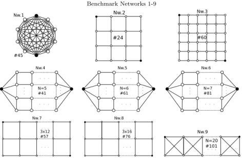
The modified approach was implemented in JAVA and tested on nine example networks on an Intel Xeon 2.97 GHz machine. Each network (nw.) in Table1is an-notated with its number of edges. The terminal nodes are colored in black. Nw.4-6 are featured with parameterN which stands for the number of horizontal edges in each row and N −1 is the number of vertical edges in each column. In nw.9, N

Procedure 2computeRel

Input: RBD Graph,List acc,EdgeProbMapepm,Stringline,FileF N ext

1: boolP orC; //Condition variable for determining path/cut 2: boolb=Graph.f indP ath();

3: if b==f alsethen

4: doubletmp=computeP roduct(acc); 5: if P orC ==truethen

6: P aths=P aths+tmp; 7: else 8: Cuts=Cuts+tmp; 9: end if 10: return 11: end if

12: SPRedred=Graph.reduce() //Preprocessing: Reduce graph. 13: epm=red.getEdgeP robM ap(); //Update edge probabilities 14: line=line+red.getString(); //Extend line with reduced terms 15: Listsp=BF S.shortestP ath(Graph); //Find shortest path 16: for eache∈sp do

17: line=line+aggregateLeaf(e); 18: end for

19: F N ext.write(line); 20: return F N ext Procedure 3bfsLevel

Input: File F P rev

1: for eachlinebranch∈F P revdo 2: //proceed each subproblem (path) 3: for eachsub∈linebranchdo

4: RBD rbd=readT askBranch(sub);

5: F N ext=computeRel(rbd, accumlation, epm, line, F N ext); 6: end for 7: end for 8: if F N ext.IsEmpty() then 9: return 10: end if 11: F P rev=F N ext; 12: F N ext= new File;

13: print ”upper bound for Unreliability = 1−P aths()”; 14: print ”lower bound for Unreliability = Cuts()”; 15: bf sLevel(F P rev);

represents the number of squares in the K4-ladder (see [2]). In order to compare the results with related papers we claim that every edge fails with a probability of 0.1 in all networks. Table 2shows the bounds computed with regard to a relative accuracy of ten percent. The last columnd(TΔ) indicates the depth or level of the

Procedure 4readTaskBranch

Input: Stringsub

1: String[] deltapath=sub.split(>); 2: for eachi∈deltapathdo

3: processN ode(deltapath[i]); //reductions

4: i=i+ 1;

5: processEdge(deltapath[i]); //merge&delete operations 6: end for

7: epm.update(); //recreated EdgeProbMap 8: acc.update(); //recreated accumlation List 9: return rbd; //reconstructed graph

delta tree after which the respective bounds were obtained. The file size, the number of tasks and the average disk IO bandwidth are also listed. It can be observed that apart from the number of components, the runtime highly depends on the structure of the network. Comparing the results of nw.3 and nw.4 in Table2 their runtimes are roughly the same. It is a wrong conclusion to expect a much faster solution for nw.4 regarding its 1.5 times higher bandwidth. The reason therefore lies in their graph structures: The shortest s-t path for nw.3 is twice as long as the one for nw.4 which means that nw.3 generates in general more subproblems in each level than nw.4. This leads to a higher computation time for processing all tasks for each level. Hence, for nw.3 more time must be spent to wait for the data to be written on hard disk leading to a lower bandwidth. Another observation concerning the im-pact of the graph structure is between nw.6 and nw.9: nw.6 has 20 components less than nw.9 but we needed about four times longer in order to achieve bounds with the same relative accuracy. Though we start with a lower number of subproblems (length of shortest s-t path) in nw.6, this number still remains high after several recursion levels for many child nodes in TΔ leading to a high number of tasks for

each level. For nw.6 272 million subproblems are stored in 21.4 GB which means that in average 84 Bytes are needed to encode a task. Comparing the bandwidth of nw.4-6, we notice that the larger the network becomes the lower the average disk bandwidth. The simple reason is that it takes more time to perform graph manipulations on larger graphs and more subproblems evolve due to the increasing length of the shortest s-t path leading to a higher latency. For some networks it was not possible to obtain the exact results within two days. Those that we could finish are listed in Table 3. dmax(TΔ) represents the maximal depth (or the total

amount of levels) of the delta tree. Note that the depth of the tree is limited by the number of edges of the original input graph since the number of edges decreases by at least one, in each recursion. d_w(TΔ) is the broadest level of the tree. The

file size of this level also indicates the maximum disk space needed for the whole computation. We can make the following observation by comparing the two tables: For large networks we only need a little fraction of the total time and also of the maximum required disk space in order to reach satisfying bounds. For example, for nw.3 the fraction of disk space required is 0.071 percent and the time spent is only 0.018 percent of the overall time. Similarly, this can be observed for nw.5.

We remark that for even smaller failure probability values - in the magnitude of 10−5 for highly reliable systems - the bounds would be obtained in an even shorter amount of time requiring less hard disk space.

To compare the implementation based on the delta tree and disk storage with an older implementation of the method [15] extended with series and parallel reduc-tions, we have added another time column. For nw.5-9 the memory of 2GB was exhausted before the respective bounds could be achieved. For all the other net-works we can observe that the runtime is shorter for the small sized nw.1 and nw.2 but it takes significantly more time for the larger networks three and four. This is due to the hold of all subgraphs and perfomed reductions in memory by method [15]: For small sized problems less memory is required to store each generated subgraph. Furthermore less subproblems evolve. As soon as the problem reaches a certain size, more storage is needed for each subgraph and also more subproblems are to be expected. Consequently the prohibitively rapid growth of memory demand leads to a negative impact on runtime.

Table 1 Benchmark Networks 1-9

5

Conclusion

In this work we stressed the problem of high memory consumption for the Gobien Dotson algorithm. Due to the exponential nature of the terminal-pair reliability problem, the demand for memory grows unacceptably with the size of the networks to be assessed. This imposes a limiting factor for reaching good reliability bounds since the computation must be interrupted because of memory shortage. Hence, we suggested to migrate the memory content to hard disk. Thedelta tree was encoded in a certain way to comply with the hard disk’s sequential read and write behavior. This method even allows interruptions since the files created until the point of interruption can be reused to continue the computation at a later time. We found

Table 2

Bounds (relative accuracy=0.1)

Nw lb ub time time[15] file(MB) #tasks øbw MB s d 1 1.99·10−9 2.05·10−9 0.68 s 0.41 s 0.14 1464 0.64 11 2 2.47·10−2 2.50·10−2 0.26 s 0.20 s 0.01 282 0.10 5 3 2.42·10−2 2.47·10−2 8.00 s 26.17 s 5.55 121,622 0.78 7 4 9.12·10−5 9.14·10−5 7.68 s 11.53 s 7.26 97,036 1.16 10 5 1.32·10−5 1.36·10−5 180 s - 183.78 2,631,226 0.60 11 6 1.88·10−6 1.91·10−6 7.73 h - 21,924.28 272,012,633 0.40 14 7 3.81·10−2 3.85·10−2 49.16 s - 54.10 697,592 0.75 8 8 4.36·10−2 4.38·10−2 1.39 h - 4,899.35 53,184,683 0.56 8 9 4.34·10−3 4.41·10−3 1.91 h - 9,011.64 50,958,418 0.78 10 Table 3 Exact results

Nw Unreliability time time[15] dmax dw file(MB) #tasks øbw MB s 1 2.00·10−9 9.79 s 6.26 s 36 20 1.65 12,574 1.99 2 2.49·10−2 0.35 s 0.17 s 9 5 0.01 282 0.10 3 2.43·10−2 12.45 h - 25 16 20,429.39 62,358,421 2.43 4 9.13·10−5 41.75 s 47.52 s 20 12 14.52 138,814 1.65 5 1.33·10−5 39.55 h - 30 20 30,613.73 203,132,939 1.43 7 3.83·10−2 0.61 h - 22 12 521.65 4,135,084 1.25

that only a small fraction of the complete runtime and the maximum required space is needed to obtain reasonable and accurate bounds. It must be said that this fact depends very much on the probability of failure of the system components and is pertinent for highly reliable systems. Most of the additional time only contributes to minor improvements of the bounds.

One may assume that by migrating the memory content to hard disk, afterwards the hard disk itself might be a bottleneck. However, by having a look at the measured bandwidth values, this is definitely not the case. On the contrary, the maximal average disk bandwidth of merely 2.43 MB/s shows that there is space for exploiting even further the writing speed of nowadays hard disks (of around 150 MB/s). In this context, we intend to parallelize the sequential algorithm and take advantage of the property that all tasksPΔ are independent.

Acknowledgement

We are very thankful to A. Bode from TU M¨unchen for supporting this work. Our thanks are also dedicated to M. Siegle from Universit¨at der Bundeswehr M¨unchen for many insightful discussions. We also thank the three anonymous reviewers for their helpful and detailed comments.

References

[1] A.Satyanarayana and M.K.Chang. Network reliability and the factoring theorem. InNetworks, vol.13, no.1, 107-120, 1983.

[2] C.Tanguy. Asymptotic mean time to failure and higher moments for large, recursive networks. In

CoRR, 2008.

[3] D.Torrieri. Calculation of node-pair reliability in large networks with unreliable nodes. InIEEE Trans. Reliability, vol.43, no.3, 375-377, 1994.

[4] F.M.Yeh, S.K.Lu, and S.Y.Kuo. Determining terminal-pair reliability based on Edge Expansion Diagrams using OBDD. InIEEE Trans. Reliability, vol.48, no.3, 234-246, 1999.

[5] S. J. Friedman and K. J. Supowit. Finding the optimal variable ordering for Binary Decision Diagrams. InSIAM Journal on Computing, vol.39, no.5, 710-713, 1990.

[6] J.M.Wilson. An improved minimizing algorithm for sum of disjoint products. In IEEE Trans. Reliability, vol.39, no.1, 42-45, 1990.

[7] K.Wood. A factoring algorithm using polygon-to-chain reductions for computing k-terminal network reliability. InNetworks, vol.15, no.2, 173-190, 1985.

[8] M.Lˆe and M.Walter. Bounds for Two-Terminal Network Reliability with Dependent Basic Events. In

Lecture Notes in Computer Science, vol.7201/2012, 31-45, 2012.

[9] M.O.Ball. Computational complexity of network reliability analysis: An overview. InIEEE Trans. Reliability, vol.35, no.3, 230-239, 1986.

[10] N.Deo and M.Medidi. Parallel algorithms for terminal pair reliability. InIEEE Trans. Reliability, vol.41, no.2, 201-209, 1992.

[11] O.R.Theologou and J.G.Carlier. Factoring and reductions for networks with imperfect vertices. In

IEEE Trans. Reliability, vol.40, no.2, 210-217, 1991.

[12] R.E.Barlow and F.Proshan.Mathematical Theory of Reliability. John Wiley & Sons, 1965.

[13] S.J.Hsu and M.C.Yuang. Efficient computation of terminal-pair reliability using triangle reduction in network management. InICC on Communications, vol.1, 281-285, 1998.

[14] S.Soh and S.Rai. Experimental results on preprocessing of path/cut terms in sum of disjoint products technique. InIEEE Trans. Reliability, vol.42, no.1, 24-33, 1993.

[15] W.P.Dotson and J.Gobien. A new analysis technique for probabilistic graphs. InIEEE Trans. Circuit & Systems, vol.26, no.10, 855-865, 1979.

[16] Y.B.Yoo and N.Deo. A comparison of algorithms for terminal pair reliability. In IEEE Trans. Reliability, vol.37, no.2, 210-215, 1988.

[17] Y.G.Chen and M.C.Yuang. A cut-based method for terminal-pair reliability. In IEEE Trans. Reliability, vol.45, no.3, 413-416, 1996.