HAL Id: hal-02112287
https://hal.archives-ouvertes.fr/hal-02112287v2
Submitted on 3 Nov 2020
HAL
is a multi-disciplinary open access
archive for the deposit and dissemination of
sci-entific research documents, whether they are
pub-lished or not. The documents may come from
teaching and research institutions in France or
abroad, or from public or private research centers.
L’archive ouverte pluridisciplinaire
HAL
, est
destinée au dépôt et à la diffusion de documents
scientifiques de niveau recherche, publiés ou non,
émanant des établissements d’enseignement et de
recherche français ou étrangers, des laboratoires
publics ou privés.
An improved branch-cut-and-price algorithm for the
two-echelon capacitated vehicle routing problem
Guillaume Marques, Ruslan Sadykov, Jean-Christophe Deschamps, Rémy
Dupas
To cite this version:
Guillaume Marques, Ruslan Sadykov, Jean-Christophe Deschamps, Rémy Dupas.
An improved
branch-cut-and-price algorithm for the two-echelon capacitated vehicle routing problem.
Comput-ers and Operations Research, Elsevier, 2020, 114, pp.104833.
�10.1016/j.cor.2019.104833�.
�hal-02112287v2�
An improved branch-cut-and-price algorithm for the
two-echelon capacitated vehicle routing problem
Guillaume Marques
∗1,2,3, Ruslan Sadykov
†2,3, Jean-Christophe Deschamps
‡1, and
R´
emy Dupas
§11
IMS, Univ. of Bordeaux, Bordeaux INP, CNRS (UMR 5218) , 351 Cours de la
lib´
eration, 33405 Talence cedex, France
2
Inria Bordeaux – Sud-Ouest , 200 Avenue de la Vieille Tour, 33405 Talence
cedex, France
3
IMB, Univ. of Bordeaux, CNRS (UMR 5251), Bordeaux INP, 351 Cours de la
lib´
eration, 33405 Talence cedex, France
23 September 2019
Abstract
In the paper, we propose a branch-cut-and-price algorithm for the two-echelon capaci-tated vehicle routing problem in which delivery of products from a depot to customers is performed using intermediate depots called satellites. Our algorithm incorporates signifi-cant improvements recently proposed in the literature for the standard capacitated vehicle routing problem such as bucket graph based labeling algorithm for the pricing problem, automatic stabilization, limited memory rank-1 cuts, and strong branching. In addition, we make some specific problem contributions. First, we introduce a new route based formula-tion for the problem which does not use variables to determine product flows in satellites. Second, we introduce a new branching strategy which significantly decreases the size of the branch-and-bound tree. Third, we introduce a new family of satellite supply inequalities, and we empirically show that it improves the quality of the dual bound at the root node of the branch-and-bound tree. Finally, extensive numerical experiments reveal that our algorithm can solve to optimality all literature instances with up to 200 customers and 10 satellites for the first time and thus double the size of instances which could be solved to optimality.
1
Introduction
In a context of economic globalization, the growth of urban population leads to an increase in freight transportation in cities. Freight transportation may deteriorate the quality of the urban environment with, for example, high noise levels, greenhouse gas emissions, and decrease of air quality. Moreover, freight transportation faces several constraints such as reduced access within cities and deliveries within time-windows. As a result, freight distribution patterns in city logistics change (Taniguchi and Thompson, 2002). In the past, customers were delivered straight from depots located on the outskirts of cities. Nowadays, transporters tend to use two-tier distribution systems. In the first tier, large urban trucks ships freight from warehouses
or production sites to intermediate distribution facilities called satellites. In satellites, freight is processed and consolidated. Freight is then loaded in small city freighters which deliver customers located in city centers.
At the strategic level, two-tier distribution systems are considered in location-routing prob-lems (Crainic et al., 2011). These are integrated probprob-lems in which we take decisions on both locating facilities and routing from open facilities. At tactical and operational levels, locations of depots and satellites are known. We plan only routing of vehicles. However, we should take routing decisions on both levels at the same time to devise cost-effective solutions in two-tier distribution systems. Such integration gave rise to two-echelon routing problems (Crainic et al., 2009). The first such problem proposed in the literature by Gonzalez-Feliu et al. (2007) is the two-echelon capacitated vehicle routing problem (2E-CVRP).
In the 2E-CVRP, we must determine the number of goods to be shipped from the depot to the satellites and from satellites to customers, and the optimal routes connecting entities in each level such that vehicle capacities are not exceeded. We aim at minimizing the sum of handling costs at satellites and transportation costs depending on the total distance traveled by all vehicles.
Recently, several exact algorithms for the 2E-CVRP have been proposed in the literature. The most efficient one by Baldacci et al. (2013) is based on an enumeration of collections of first-level routes. Thus, it can efficiently tackle only instances with a small number of satellites (up to six). Moreover, this algorithm solves to optimality instances with up to 100 customers whereas the best exact algorithms for other vehicle routing problems can handle up to 300 customers (Pecin et al., 2017a). Santos et al. (2015) proposed the only branch-cut-and-price algorithm in the literature for the 2E-CVRP. This algorithm can be used to solve instances with a larger number of satellites, but experimentations show that it is less efficient than the one of Baldacci et al. (2013).
In this paper, we propose an improved branch-cut-and-price (BCP) algorithm for the 2E-CVRP which is built on recent advances for the classical capacitated vehicle routing problem (CVRP). To further improve the efficiency of our BCP algorithm, we propose the following problem-specific enhancements:
• A new route based formulation for the problem which does not involve variables which explicitly define product flow in satellites. New level balancing constraints guarantee flow conservation in satellites.
• A new family of inequalities to improve the quality of the linear programming (LP) relax-ation of the formulrelax-ation. These inequalities are inspired by the depot capacity constraints introduced for the capacitated location-routing problem by Belenguer et al. (2011).
• A new branching strategy which uses variables defining the number of urban trucks visiting a subset of satellites.
To improve the current primal bound, we employed a column generation based heuristic in the course of the algorithm. Our BCP algorithm with the embedded heuristic outperformed largely the state-of-the-art exact approach by Baldacci et al. (2013) for the problem, since it solved to optimality all instances available in the literature with up to 200 customers and 10 satellites.
Finally, we generated a new set of large instances for the problem to inspire further re-search on the 2E-CVRP. This set involves instances with up to 300 customers and 15 satellites. These instances are derived from ones recently proposed by Schneider and L¨offler (2019) for the capacitated location-routing problem.
The remaining of the paper is organized as follows. Section 2 reviews the literature. Section 3 describes the standard and the new formulations of the problem. Section 4 introduces the new family of satellite supply inequalities. Section 5 describes the proposed branch-cut-and-price algorithm. Section 6 reveals and discusses the computational results. Section 7 concludes and presents further research perspectives.
2
Literature review
Gonzalez-Feliu et al. (2007) first considered the 2E-CVRP. They proposed a freight-flow formu-lation enhanced by two families of valid inequalities. Their branch-and-cut algorithm solved to optimality instances with up to 22 customers and 2 satellites. Perboli et al. (2011) improved these results. The authors strengthened the formulation with one family of valid inequalities. They solved to optimality some instances with 33 customers. Two matheuristics were also sug-gested. They found feasible solutions to instances up to 50 customers with 10% of average gap from the lower bound.
Later, Jepsen et al. (2013) pointed out that the formulation in (Perboli et al., 2011) is not correct for instances with more than two satellites. They proposed an alternative formulation that combines the relaxation of the split-delivery CVRP by Belenguer et al. (2000) for the first level and the model for the capacitated location routing problem by Contardo et al. (2013) for the second level. Although this formulation is an outer approximation, its LP relaxation is stronger than one of Perboli et al. (2011). Since this formulation has an exponential number of constraints, the authors used a branch-and-cut algorithm. A specialized branching scheme was employed to cut non-feasible integer solutions. This approach solved to optimality instances with up to 50 customers and 5 satellites. It remains the best branch-and-cut algorithm for the problem in the literature.
Contardo et al. (2012) proposed another branch-and-cut algorithm for the two-echelon ca-pacitated location-routing problem. This problem is a generalization of the 2E-CVRP in which there are several depots and opening costs for satellites. Their branch-and-cut algorithm solved to optimality instances with up to 50 customers and 10 potential satellites.
Santos et al. (2015) proposed the first branch-cut-and-price algorithm for the 2E-CVRP. They considered a route based formulation strengthened by some valid inequalities from the CVRP literature. First-level routes are enumerated whereas second-level routes are priced by the shortest path problem with resource constraints. The pricing problem generates non-elementarity routes. They used branching strategies in the following priority order: (1) branching on the number of vehicles traveling on a first-level route, (2) branching on the number of second-level vehicles starting from a satellite, and (3) branching on the use of an arc by a second-level route. The computational results of Santos et al. (2015) were similar to those by Jepsen et al. (2013).
The exact approach by Baldacci et al. (2013) also uses a route based formulation. The method is based on an intelligent enumeration of collections (i.e. subsets) of first-level routes. Authors devised lower and upper bounding procedures to limit the number of collections which may lead to an optimal solution. By fixing a subset of first-level routes, the problem is reduced to the multi-depot capacitated vehicle routing problem with limited depot capacities. The latter was solved by an adaptation of the algorithm by Baldacci and Mingozzi (2009). Computational experiments showed that the overall approach outperforms the one by Jepsen et al. (2013). Baldacci et al. (2013) could solve instances with up to 100 customers and 5 satellites. Their approach remains the best exact algorithm in the literature until now. However, the fact that collections of first-level routes are enumerated does not allow one to employ this approach for instances with 10 satellites or more.
There are several heuristic approaches for the 2E-CVRP in the literature. Hemmelmayr et al. (2012) proposed an adaptive large neighborhood search based heuristic that works for both 2E-CVRP and the location-routing problem. It largely improved the best feasible solutions found by Perboli et al. (2011). Moreover, the authors proposed a new test set of instances with up to 200 customers and 10 satellites.
Zeng et al. (2014) suggested a hybrid heuristic which is composed of a greedy randomized adaptive search procedure (GRASP) with a route-first cluster-second procedure embedded in a variable neighborhood descent (VND). Breunig et al. (2016) developed an improved large neighborhood-based hybrid meta-heuristic. It combines enumerative local search with destroy-and-repair principles, as well as some tailored operators to optimize the selections of satellites. Both these approaches improved the best-known solutions for many instances.
Recently, two matheuristics were proposed in the literature. Wang et al. (2017) employed a mixed-integer mathematical model for the 2E-CVRP, in which arc variables are used for the first level, and path variables for the second level. They used variable neighborhood search to construct the set of second-level routes, and they then solved the mathematical model to improve the obtained solution. The authors improved 13 best-known solutions. Finally, Amarouche et al. (2018) used a similar approach in which a pool of routes is collected by a local search heuristic combined with a destroy-and-repair method. Then, the route based formulation is solved with the hope to improve the best solution found so far. This approach improves 7 best-known solutions for the largest instances of the 2E-CVRP.
Further information can be found in the survey on two-echelon routing problems by Cuda et al. (2015).
3
Formulation
Let us now formally define the problem. At the first level, a setKof homogeneous urban trucks ships freight from a depot denoted as 0 to a set S of intermediate depots called satellites. At the second level, a set Lof homogeneous city freighters picks freight at satellites and deliver it to a set C of customers. Each vehicle must return to the place from where it started its tour (depot for urban trucks and satellites for city freighters). Urban trucks have a capacity of Q1
items, and city freighters have a capacity of Q2 items. A satellites∈ S can hold up toLs city
freighters and charges fsH for each processed item of freight. Each customer c ∈ C asks for dc
items of freight and must be visited exactly once. At each satellite, the total amount of freight delivered by urban trucks must be equal to the amount of freight picked by city freighters that start at this satellite. The objective of the problem is to minimize the sum of handling costsfH and transportation costsfT.
We use the route based formulation to model the problem. The first level is similar to the split-delivery CVRP since several urban trucks can supply a satellite. However, the amount of freight delivered to each satellite is not known. A complete undirected graph G1 = (V1, E1),
V1 ={0} ∪ S, represents the first level of the distribution system. LetP be the set of feasible
first-level routes and let ˜zpe∈Ndenote the number of times pathp∈P uses edgee∈E1.
The second level corresponds to the multi-depot CVRP where depots are satellites. Each customer is visited by one city freighter, and each satellite cannot supply more freight than the amount delivered to it by urban trucks. This level is represented by an undirected graph G2 = (V2, E2) where V2 =C ∪ S and E2 ={(i, j) | i∈ S ∪ C, j ∈ C, i6=j}. For any satellite
s ∈ S, letRs be the set of feasible second-level routes starting and finishing ins. We denote
R=∪s∈SRs. A second-level router∈Ris described by vector ˜xrwhere element ˜xre∈Ndenotes
the number of times routeruses edgee∈E2. We also introduce vector ˜yrwhere element ˜yrc ∈N
denotes the number of times routervisits customerc∈ C. Given graphGi,i= 1,2, we denote
as δi(v) the set of edges inEi incident to vertexv∈Vi.
The cost of traversing edge e ∈ E1∪E2 is denoted by feT. From now on, we make two
assumptions. First, transportation costsfT satisfy the triangle inequality. Otherwise, we
trans-form the instance to an equivalent one: if the minimum cost path between two vertices v, v0 passes by other vertices, we set the cost f(v,vT 0) to the cost of the minimum path. The second
assumption is that transportation costs are symmetric. If this is not the case, graphs G1 and
G2become directed ones, edges become arcs, and all values ˜ze=(v,v0)and ˜xe=(v,v0)depending on
edges are replaced by sums of values ˜za=(v,v0)+ ˜za=(v0,v)and ˜xa=(v,v0)+ ˜xa=(v0,v)depending on
arcs. All instances in the 2E-CVRP literature satisfy these two assumptions.
3.1
Standard formulation
We now describe the standard route based formulation for the 2E-CVRP. It was proposed by Bal-dacci et al. (2013) and used in Santos et al. (2015); Amarouche et al. (2018). Integer variable
λp is equal to the number of urban trucks traveling on first-level routep∈P. We denote as Sp
the set of satellites visited by route p∈P: Sp ={s∈ S : Pe∈δ1(s)z˜
p
e = 2}. We denote as PS
the set of first-level routes visiting at least one satellite in S⊆ S: PS ={p∈P : Sp∩S6=∅}.
Continuous variablewpsis equal to the amount of freight that first-level routep∈P{s} delivers
to satellite s∈Sp. Binary variable µr is equal to one if and only if a city freighter travels on
second-level route r ∈ R. To simplify the presentation, we introduce the continuous auxiliary variablebsthat is equal to the total amount of freight delivered to satellites∈ S.
(F1) min X p∈P X e∈E1 feTz˜epλp+ X r∈R X e∈E2 feTx˜reµr+ X s∈S fsHbs (1) s.t. X r∈R X c∈C ˜ ycrµr= 1 c∈ C (2) X r∈Rs µr≤Ls s∈ S (3) X r∈R µr≤ |L| (4) X p∈P λp≤ |K| (5) X s∈Sp wps≤Q1λp p∈P (6) bs= X p∈P{s} wps s∈ S (7) bs= X r∈Rs X c∈C dcy˜crµr s∈ S (8) λp∈N p∈P (9) µr∈ {0,1} r∈R (10) wps≥0 p∈P, s∈Sp (11)
Objective function (1) minimizes the sum of transportation and handling costs. Constraints (2) ensures each customer is visited by exactly one second-level route. Constraints (3), (4), and (5) are upper bounds on the number of used vehicles. Constraints (6) make sure that the capacity of urban trucks is not exceeded. Constraints (7) and (8) ensure the flow balance between the two distribution levels. Constraints (9), (10) and (11) define domains of variables.
3.2
Modified formulation
In F1, we use variablewtogether with constraints (6) and (7) to ensure the flow balance between two distribution levels. To obtain the modified formulation, we project F1 to the space of variablesλandµonly. Investigation of this kind of projection for the CVRP has been performed by Letchford and Salazar-Gonz´alez (2006). To simplify the presentation, we introduce auxiliary integer variablesuS that define the number of urban trucks visiting a non-empty subsetS ⊆ S
of satellites. The modified formulation is then (F2) min X p∈P X e∈E1 feTz˜epλp+ X r∈R X e∈E2 feTx˜reµr+ X s∈S fsHbs s.t. X r∈R X c∈C ˜ yrcµr= 1 c∈ C X r∈Rs µr≤Ls s∈ S
X r∈R µr≤ |L| X p∈P λp≤ |K| bs= X r∈Rs X c∈C dcy˜crµr s∈ S uS = X p∈PS λp S⊆ S, S6=∅ (12) X s∈S bs≤Q1uS S⊆ S, S6=∅ (13) λp∈N p∈P µr∈ {0,1} r∈R
Constraints (12) define variablesu. Level balancing constraints (13) replace variableswand constraints (6), (7), (11). We now prove that F2 is a projection of F1. The proof is illustrated in Figure 1.
Proposition 1. A solution (¯λ,µ)¯ is feasible for the LP relaxation (LF2) of formulation F2 if
and only if there exists a feasible solution (¯λ,µ,¯ w)¯ for the LP relaxation (LF1) of formulation F1.
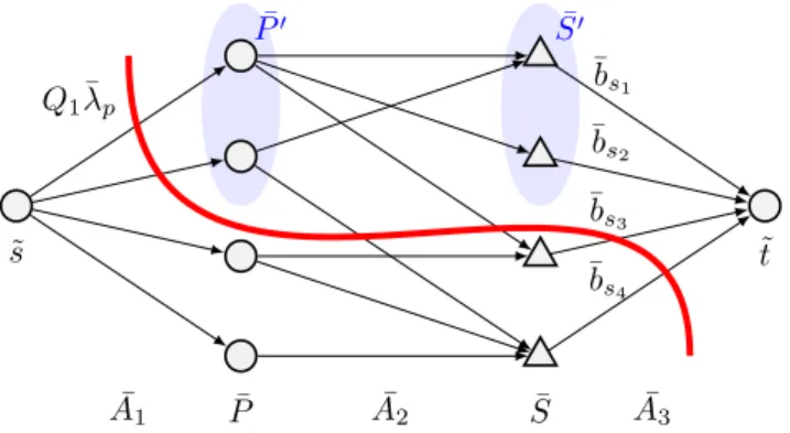
Proof. We first prove necessity, i.e “only if” part. Given a solution (¯λ,µ) for F2 and its computed¯ values (¯b,u), we construct a directed graph ¯¯ G= ( ¯V ,A). Set ¯¯ V of nodes contains source ˜s, sink ˜
t, set ¯P ={p∈ P : ¯λp > 0} of nodes representing first-level routes in the solution, and set
¯
S ={s∈ S: ¯bs>0} of nodes representing satellites used in the solution. Set ¯A of arcs is the
union of the following three sets: ¯A1connects the source with ¯P, ¯A2connects ¯P with ¯S, and ¯A3
connects ¯S with the sink. An arc (˜s, p) in ¯A1has capacityQ1¯λp. An arc (p, s) belongs to ¯A2 if
and only ifs∈Sp and has infinite capacity. An arc (s,˜t) in ¯A3has capacity ¯bs.
Let us now prove by contradiction that the maximum value of the ˜s- ˜t flow in graph ¯G is equal toP
c∈Cdc=d(C). Suppose that the maximum flow is strictly less thand(C). Let ¯V0 be
the subset of ¯V obtained from a minimum ˜s-˜tcut in ¯G, ˜s∈V¯0. Let ¯S0 = ¯S\V¯0 and ¯P0= ¯P\V¯0.
We denote as δ( ¯V0) ={(v, v0)∈A¯|v ∈V¯0, v0 6∈V¯0} the set of arcs forming the minimum cut. From the supposition and the max-flow-min-cut theorem it follows that the total capacity of δ( ¯V0) is less thand(C). Thusδ( ¯V0) contains at least one arc in ¯A1and does not contain all arcs
in ¯A3. Therefore, the total capacity of arcs in ¯A1∩δ( ¯V0) is strictly less than the total capacity
of arcs in ¯A3\δ( ¯V0): X p∈P¯0 Q1λ¯p< X s∈S¯0 ¯bs. (14)
Setδ( ¯V0) does not contain any arc in ¯A2 as they have infinite capacity. Thus ¯V0∩P¯∩PS¯0
is empty, and ¯λp = 0 for allp∈PS¯0\P¯0. From the latter and (14), it follows thatPs∈S¯0¯bs>
Q1Pp∈PS¯0
¯
λp which violates constraints (12) and (13) for set ¯S0 of satellites. Thus (¯λ,µ) is not¯
a feasible solution for LF2 which leads to a contradiction.
We have just proved that the maximum flow in graph ¯G has value d(C). We now set ¯wps
equal to the flow fromp∈P¯ tos∈S¯for every (p, s)∈A¯2, and to 0 otherwise. By construction
of graph ¯G, constraints (6) and (7) are satisfied by (¯λ,¯b,w), and (¯¯ λ,µ,¯ w) is a feasible solution¯ for LF1.
To show the sufficiency (“if” part), we prove that constraints (13) are valid for LF1. If (¯λ,µ,¯ w) is feasible for LF1, then for an arbitrary subset of satellites¯ S⊆ S,S6=∅, we have
X s∈S ¯bs(7)=X s∈S X p∈P{s} ¯ wps= X p∈PS X s∈Sp ¯ wps (6) ≤ X p∈PS Q1λ¯p (12) ≤ Q1uS.
Thus, (¯λ,µ) is feasible for LF2.¯ Q1λ¯p ¯bs 1 ¯b s2 ¯b s3 ¯bs 4 ˜ s ˜t ¯ P S¯ ¯ A1 A¯2 A¯3 ¯ S0 ¯ P0
Figure 1: Illustration for graph ¯Gand its minimum cut in Proposition 1.
The main advantage of formulation (F2) is a significantly smaller number of variables. This comes at the cost of an additional exponential set of constraints (12) and (13). However, these constraints can be separated in polynomial time as showed in the proof of Proposition 1. In the separation procedure, we search for a minimum cut in graph ¯G constructed from a fractional solution (¯λ,µ) of (F2). Once set ¯¯ S0of satellites is found, it is further separated into subsets such that there is no path in ¯P visiting two satellites in different subsets. Then, we add constraints (12) and (13) for every such subset of satellites.
An additional potential advantage of formulation (F2) is the possibility to generate variables λpdynamically, similarly to variablesµ. Dynamic generation ofλis necessary when the number
of satellites is large. We do not do it in our work, as we consider instances with at most 15 satellites. Instead, we enumerate all the first-level routes. In this procedure, for each subset S⊆ S of satellites, we solve the traveling salesman problem in which we find the shortest route starting and finishing at the depot 0 and visiting all satellites inSexactly once. Then, we assign each first-level route to aλvariable, and we add all first-level route variablesλto the formulation before starting the algorithm. Thus, the formulation contains 2|S|−1 first-level route variables. All exact algorithms in the literature for the 2E-VRP use enumeration of first-level routes.
3.3
Valid inequalities
In our BCP algorithm, we use four families of valid inequalities. In this section, we present the first three families. To simplify the presentation, we introduce auxiliary variablesxand y:
xse= X r∈Rs ˜ xreµr, s∈ S, e∈E2, ycs= X r∈Rs ˜ yrcµr, s∈ S, c∈ C.
Integer variablexseis equal to the number of times edgee∈E2is used by city freighters started
from satellites∈ S. Binary variable ys
c is equal to one if and only if customer c∈ C is visited
by a city freighter started from satellites∈ S.
3.3.1 Rounded capacity cuts
Rounded capacity cuts were introduced by Laporte and Nobert (1983) for the CVRP. Term
dd(C)/Q2e is a lower bound on the number of city freighters which have to visit at least one
customer in C. Therefore, the next rounded capacity cuts (RCC) are valid: X s∈S X e∈δ2(C) xse≥2 d(C) Q2 , C⊆ C. (15)
Constraints (15) are separated using the CVRPSEP package (Lysgaard, 2018) which implements the heuristic by Lysgaard et al. (2004).
3.3.2 Chv´atal-Gomory rank-1 cuts
Here we consider Chv´atal-Gomory rounding of set-partitioning constraints (2) relaxed to ≤
inequalities. Consider a vector α of multipliers such thatαc ≥0, c ∈ C. Then, the following
rank-1 cut (R1C) is valid: X s∈S X r∈Rs $ X c∈C αcy˜rc % µr≤ $ X c∈C αc % . (16)
An inequality (16) obtained using a vector of multipliers with l positive components is called anl-row rank-1 cut. If all positive components ofαare the same, the corresponding inequality is called a subset-row cut. Jepsen et al. (2008) first introduced 3-row subset-row cuts. Pecin et al. (2017a) usedl-row subset-row cuts withl≤5. Generall-row rank-1 cuts withl≤5 were considered by Pecin et al. (2017b). They determined all dominant vectors of multipliers for such cuts: if an l-row rank-1 cut with l ≤ 5 is violated, at least one rank-1 cut obtained using a dominant vector of multipliers is violated.
Similarly to Sadykov et al. (2017), separation of l-row rank-1 cuts with l ≤5 is performed using a local search heuristic separately for every dominant vector of multipliers. We employ the limited memory technique by Pecin et al. (2017a) to reduce the impact of rank-1 cuts on the solution time of the pricing problem.
3.3.3 Visited satellite inequalities
A customer can be visited by a route r∈Rs only if satellite sis visited by at least one urban
truck. Therefore, next visited satellite inequalities (VCI) are valid:
ycs≤u{s}, c∈ C, s∈ S. (17)
Although inequalities (17) are rather straightforward, we did not find any work in the literature which uses them. Separation of constraints (17) is performed by enumeration of all pairs (c, s)∈
C × S.
3.3.4 Lower bounds on the number of vehicles
We define lower bounds on the number of urban trucks
X p∈P λp≥ d(C) Q1 (18) and the number of city freighters
X r∈R µr≥ d(C) Q2 (19)
Moreover, a subset S of satellites must be visited by enough urban trucks to supply the demand that cannot be delivered from satellites in S \S. Therefore, the next lower bound on uS is valid : uS ≥ & d(C)−P s∈S\SLsQ2 Q1 ' , S⊂ S (20)
Inequalities (20) are useful when the number of city freighters that can start from satellites is limited (Ls<|L|, s∈ S).
4
New family of valid inequalities
We propose a new family of satellite supply inequalities (SSI) inspired by the depot capacity constraints introduced for the capacitated location-routing problem by Belenguer et al. (2011). To simplify the presentation below, we denoteC{=C \C andS{=S \S. Let us introduce SSI using an example.
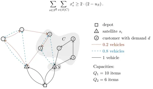
Example 1. Consider urban trucks with capacity Q1 = 10 and city freighters with capacity
Q2 = 6. Figure 2 shows a fractional solution (¯u,µ)¯ for LF2. Here S = {s1, s2} and set C
contains seven customers. Consider subsetCof customers withd(C) = 11. Consider also subset S ={s2} of satellites with u¯S = 1. Clearly,S can supply only demand of at most Q1u¯S = 10
units and thus cannot supply set Cof customers alone. In this fractional solution, Cis supplied by 1.8 city freighters coming from S and 0.2 city freighters coming from S{. The violated SSI states that either two or more urban trucks should visit S ={s2} or at least one city freighter
coming from satellites in S{={s1} should visit some customers inC:
X s∈S{ X e∈δ(C) xse≥2·(2−uS). C S 3 2 1 2 3 1 2 depot i satellitesi
d customer with demandd
0.2 vehicles 0.8 vehicles 1 vehicle Capacities: Q1= 10 items Q2= 6 items
Figure 2: Example of a satellite supply inequality, violated for givenS andC.
4.1
Satellite supply inequalities
We now definegC(u) as the function which gives a lower bound on the number of city freighters
required to cover the demand of a subsetC of customers thatbucurban trucks cannot supply:
gC(u) = max 0, d(C)−Q 1buc Q2 .
Proposition 2. Given C⊂ C andS ⊂ S, the following inequality is valid for the 2E-CVRP
X
s∈S{ X
e∈δ2(C)
xse≥2·gC(uS). (21)
Proof. Consider a feasible solution (¯x,¯b,u) of formulation (F2). The following rounded capacity¯ inequality is satisfied by ¯xand ¯b:
X s∈S{ X e∈δ2(C) ¯ xse≥2 d(C)−P s∈S¯bs Q2 (22)
From constraint (13) and the integrality of variable ¯uS, it follows
X
s∈S
¯
bs≤Q1¯uS =Q1bu¯Sc. (23)
By combining (22) and (23) we obtain that (21) is satisfied by ¯xand ¯u.
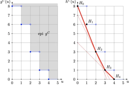
FunctiongC(u) is not linear and cannot be used directly. Instead, we use the piecewise linear
function, denoted ashC(u), which forms the convex hull of the epigraph ofgC(u). We denote as
˜
uC the ordered vector of (integer) valuesuof extreme points ofhC:
˜
uC =u˜C0 = 0,u˜C1, . . . ,u˜Ck(C)=dd(C)/Q1e
.
Figure 3 depicts an example of functions gC and hC forQ1 = 10, Q2= 4, and d(C) = 32. In
the left plot, the epigraph of gC is the grey area. In the right plot, function hC is the bold
line. Extreme points of hC are H
0, H2, H3, H4, but not H1. Therefore, ˜uC = (0,2,3,4), and
k(C) = 3.
Figure 3: Example of functionsgC (on the left) andhC (on the right).
Proposition 3. Given subsets C ⊂ C, S ⊂ S, and an integer 0 < k ≤ k(C), the following
inequality is valid for the 2E-CVRP X s∈S{ X e∈δ2(C) xse≥2· hC(˜uCk−1)−h C(˜uC k−1)−h C(˜uC k) ˜ uC k −u˜Ck−1 (uS−u˜Ck−1) ! (24)
Proof. The right-hand side of each constraint (24) corresponds to a linear piece of functionhC.
Thus the proof follows from Proposition 2 and from the fact thathC(u)≤gC(u) for allu≥0.
4.2
Separation of SSI
Let (¯x,u) be the values of variables¯ xanduin a solution for LF2. The following problem finds the most violated inequality.
max S⊂S,C⊂C2·h C(¯u S)− X s∈S{ X e∈δ2(C) ¯ xse (25)
The first and second terms of the objective function are non-linear functions of C and S. Thus enumeration of C and S is required to compute (25) exactly using an integer program. Since the number of subsets is exponential, we propose a heuristic to separate SSI. Although the heuristic does not necessarily find the most violated inequality, it offers a good trade-off between the computational effort and the violation of found inequalities. Our heuristic works with a fixed set of satellites. The following proposition gives a dominance rule which will allow us to discard non-interesting subsets of satellites.
Proposition 4. Consider a solution (¯x,u)¯ for LF2 and a fixed set C of customers. If SSI (24)
is violated for C and a set S1 of satellites, then it is violated for C and any set S2 ⊇S1 such
that u¯S2= ¯uS1.
Proof. The right-hand side of (24) is fixed for a fixed setC of customers and a fixed valueuS.
Thus right-hand side of the SSIs for pairs (C, S1) and (C, S2) is the same. For fixed values of
variables x, the left-hand side of the SSI for pair (C, S2) is not larger than one of the SSI for
pair (C, S1), asS{2 ⊆S1{. Thus the violation of the SSI for pair (C, S2) is not smaller than one
of the SSI for pair (C, S1).
To enumerate all the non-dominated sets of satellites, we first build the power set ¯U of set ¯S of satellites used in the solution. Since we look for the largest subsets of satellites, we append all satellites in S \S¯ to each set in ¯U. Finally, we exclude from ¯U all sets S1 such that there
exists S2∈U¯ withS2 ⊇S1 and ¯uS2 = ¯uS1. This is done by the exhaustive enumeration as the cardinality of set ¯U is not large for the instances of the literature.
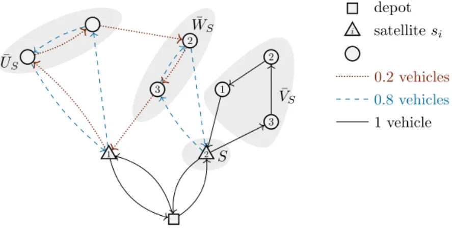
¯ VS S ¯ US ¯ WS 3 2 1 2 3 1 2 depot i satellitesi 0.2 vehicles 0.8 vehicles 1 vehicle
Figure 4: Separation graph ¯G2(S) for the fractional solution in Example 1
Given a setS ∈ U¯ of satellites, we now look for subsets of customers that violate SSI. We split customers in three subsets. Let ¯US ⊂ C be the set of customers visited only by routes
started from S{, let ¯VS ⊂ C be the set of customers visited only by routes started fromS, and let ¯WS =C \( ¯US∪V¯S). Figure 4 illustrates the partition of customers of Example 1. We then
build graph ¯G2(S) in the following way.
• Graph ¯G2(S) is the subgraph of G2induced by vertices in ¯US∪W¯S∪S{.
• Weight of each edgeein ¯G2(S) is equal toPs∈S{x¯se.
• Set ¯US∪S{ of vertices in ¯G2(S) is merged into one vertex ¯sby successively contracting all
edges having two incident vertices in ¯US∪S{. Weight of each edge (¯s, c),c∈W¯S, in final
graph ¯G2(S) is then equal toPs∈S{ P
i∈U¯S∪S{x¯s(i,c).
Afterwards, we compute the minimum cut in ¯G2(S). Let ¯CS be the subset of vertices obtained
from the minimum cut, ¯s6∈C¯S. First, we verify whether SSI based on setS of satellites and set
and check the violation of SSI based on S and C at each iteration. Customer c0 to include in current set C(and exclude from ¯WS) in each iteration is
c0= arg max c∈W¯S ( P s∈S{dcy¯cs P s∈S{ P i∈U¯(S,C,c)¯xs(c,i) ) , (26)
where ¯U(S, C, c) =S{∪U¯S∪W¯S\ {c}. The intuition behind (26) is that we try to increase the
first term of (25) while increasing not too much the second term. The separation procedure is formally given in Algorithm 1.
Algorithm 1Separation procedure for the satellites supply inequalities
We are given (¯λ,µ) and computed entities ¯¯ P, ¯u, ¯x, ¯y
I is the set of found violated SSI
Find set ¯U of non-dominated subsets of satellites
for allS∈U¯ do
Find ¯US, ¯VS, ¯WS and build graph ¯G2(S)
Compute the minimum cut in ¯G2(S) and corresponding set ¯CS
C←C¯S∪V¯S
repeat
If SSI based onS andC is violated by (¯u,x), add the inequality to¯ I
Find customerc0 in ¯WS using (26)
C←C∪ {c0}
¯
WS ←W¯S\ {c0}
untilW¯S=∅
end for
Return a specified number of the most violated SSI inI
We now analyse the complexity of Algorithm 1. The cardinality of set ¯U is at most 2|S¯|, as
well as the number of iterations in the separation algorithm. Construction of graph ¯G2(S) takes
at most|S¯| · |C|2 operations. Computing the minimum cut has complexityO(|C|3). The number
of iterations of the internal loop is at most|C|, and the complexity of each iteration is|S¯| · |C|2.
Thus, the overall complexity of the separation algorithm isO 2|S¯|· |S¯| · |C|3 .
5
Branch-Cut-and-Price algorithm
Formulation F2 together with valid inequalities RCC, R1C, VCI, and SSI is solved by an adap-tation of the branch-cut-and-price algorithm proposed by Sadykov et al. (2017). In this section, we describe the main ingredients of this algorithm. The reader is invited to consult the original paper for all details.
As the number of variables depends exponentially on the number of satellites and customers, LF2 (called the master problem) is solved by the column and cut generation approach.
5.1
Pricing problem
Second-level route variables µ are dynamically generated by solving the pricing problem. It is decomposed into|S|subproblems (SPs), one per satellites∈ S. The set of feasible solutions for
SPsis the setRs of paths in graphG2. A pathrbelongs toRs if and only if :
• it starts and finishes in vertexs: P
e∈δ2(s)x˜
r e= 2;
• it does not pass through other satellites: P
e∈δ2(S\{s})x˜
r e= 0;
• its total delivered demand does not exceed the capacity of a city freighter: P
c∈Cy˜cr≤Q2.
Let π, ψ, φ, ρ, τ, θ, ξ, and ζ be optimum dual values for the master problem restricted to a subset of variables µ. These dual values correspond to constraints (2), (3), (4), (8), (15), (16), (17), and (24). Let alsoK be the collection of active rank-1 cuts corresponding to vectors (αk)k∈K, and Ms be the collection of active SSI based on sets (Sm, Cm)m∈Ms, s ∈ S
{
m. The
reduced cost of a pathr∈Rsis then equal to
X e∈E2 feT − X C∈C: e∈δ(C) τC− X m∈Ms: e∈δ2(Cm) ζm ˜ xre −X c∈C X e∈δ2(c) 1 2(πc+dcρs−ξ s c) ˜x r e+ X k∈K θk $ X c∈C αcky˜cr % +ψs+φ. (27)
When rank-1 cuts (16) are absent, a path has a reduced cost that is equal to the sum of reduced costs of its edges. In this case, pricing subproblem SPs is the resource constrained
elementary shortest path problem. This problem can be time-consuming to solve. Therefore, we relax the elementarity constraint and work withng-paths (Baldacci et al., 2011). This relaxation has an impact only on the optimum value of LF2. The validity of F2 is preserved. For each customer, itsng-neighborhood is static and includes 8 closest customers including itself.
Presence of active rank-1 cuts makes the pricing problem more complicated because each such cut adds a resource to the problem. To limit the increase in difficulty of the pricing problem, we use the limited memory technique proposed by Pecin et al. (2017a). For each cut (16) a memory is associated. It consists of a subset of edges inE2. This memory makes the resource associated
to the cut local: we need to track its consumption only in a small part of the graph.
Each pricing subproblem SPs is solved by the bucket graph based bi-directional labeling
algorithm proposed by Sadykov et al. (2017). This algorithm supports bothng-path relaxation and presence of dual values associated with limited-memory rank-1 cuts. If the transportation costsfT are symmetric, the algorithm exploits the forward-backward path symmetry.
5.2
Column and cut generation
We use three-stage column generation to speed up convergence. In the first two stages, the pricing problem is solved by the same heuristic labelling algorithms as in (Sadykov et al., 2017). In the last stage, the pricing problem is solved by the exact labelling algorithm. For each subproblem, heuristic pricing generates at most 30 columns, and exact pricing generates at most 150 columns. We also apply automatic dual pricing smoothing stabilization suggested by Pessoa et al. (2018) to further speed-up the convergence of column generation.
We use the bucket arc elimination procedure (Sadykov et al., 2017). It reduces the size of graph G2 by removing arcs which are proved to be absent from any improving solution to the
problem. The procedure is first performed after the first column generation convergence, and then each time the primal-dual gap decreases by more than 10%. Note that graph reduction is not the same in different pricing subproblems.
After each call to the bucket arc elimination procedure, we use the elementary route enu-meration technique by Baldacci et al. (2008). For each pricing subproblem, this procedure tries to enumerate all elementary routes with reduced cost smaller than the current primal-dual gap. If the enumeration succeeds, the pricing subproblem is solved by inspection in future column generation iterations, similarly to Contardo and Martinelli (2014). If the total number of enu-merated routes in all subproblems is less than 5000, all the routes are added to formulation F2 and the latter is solved by the MIP solver.
We define variables uonly for subsets with 5 satellites or less in order to limit the size of the formulation and reduce the number of candidates for branching. Moreover, for every subset
S such that|S| ≥6, we replace variableuS by expression t1−Pp6∈PSλp, wheret1 is the total
number of urban trucks used. This replacement allows us to keep the coefficient matrix sparse. In the beginning, all constraints (13) are added to formulation F2 for instances with at most 10 satellites. For instances with 15 satellites, only constraints (13) for setsS ⊂ S,|S| ≤5, are added. Other constraints are dynamically separated as described in Section 3.2.
In each cut generation round, we add at most 100 rounded capacity cuts (15), 450 rank-1 cuts (16), 50 VCI (17), and 150 SSI (24) to the master problem. The cut generation is stopped either by the tailing-off condition or when the time spent to solve at least one pricing subproblem exceeds 1 second. The tailing-off condition is satisfied when after 3 cut generation rounds the primal-dual gap decreases by less than 2% per round.
The parameterisation of column and cut generation is inherited from the BCP algorithm in Sadykov et al. (2017).
5.3
Branching
We perform branching on: the number of first-level routes visiting a subset of satellites (variables u), the use of first-level routes (variablesλ), the use of an edge inE2(variablesx), the assignment
of a customer to a satellite (variabley), the number of first-level routes (P
p∈Pλp), the number
of second-level routes (P
r∈Rµr), and the number of second-level routes started from a satellites
(P
r∈Rsµr). We use a multi-phase strong branching procedure, similar to Sadykov et al. (2017),
to choose the most promising branching candidate.
The branching procedure first chooses at most 50 branching candidates. Up to half of the candidates are chosen according to the branching history using pseudo-costs. In the first phase, we solve the LP relaxation of the restricted master problem. Three candidates with the largest product of lower bound improvements in the branches are chosen for the next phase. In the second phase, column generation is performed, but the pricing problem is solved with only heuristic labeling algorithms. The best candidate is chosen using the same product rule. In the third phase, the exact column and cut generation is performed in both branches of the chosen candidate using the same parameters as in the root node.
5.4
Primal heuristic
After each node in the branch-and-bound tree, a heuristic looks for improving feasible solutions to the 2E-CVRP. We first tried the standard restricted master heuristic (Sadykov et al., 2018) in which the MIP solver solves the current restricted master problem. However, we have not been satisfied with the performance of this heuristic, especially for instances with large capacity of city freighters. The reason is that sometimes only a small part of columns in the restricted master are elementary, thus making the solution space of the restricted master very small or even empty.
Instead, we use the heuristic based on an artificial primal bound and the elementary route enumeration, similar to Pessoa et al. (2009). In an iterative procedure, we decrease the artificial bound in order to divide the primal-dual gap by two in each iteration. Then, we perform elementary route enumeration for each pricing subproblem. The iterative procedure stops when the enumeration succeeds for all subproblems. Afterward, we pick 10000 elementary routes with the smallest reduced cost and add them to the master problem. Finally, we let IBM CPLEX MIP solver to solve the resulting problem with the time limit of |C|/2.5 seconds. We activate the polishing heuristic (Rothberg, 2007) implemented in CPLEX.
6
Computational Results
The implementation of proposed algorithm is done using VRPSolver by Pessoa et al. (2019), which is available at https://vrpsolver.math.u-bordeaux.fr for free academic use. This solver includes the following components:
• BaPCod C++ library (Vanderbeck et al., 2019) which implements the BCP framework;
• C++ code, developed by Sadykov et al. (2017), which implements the bucket graph based labeling algorithm, bucket arc elimination procedure, elementary route enumeration, and the separation algorithm for R1C;
• CVRPSEP C++ library (Lysgaard, 2018) which implements heuristic separation of RCC. IBM CPLEX Optimizer version 12.8.0 is used as the LP solver in column generation and as the solver for the enumerated MIPs.
To reproduce the results, it suffices to i) define models F1 and F2; ii) to implement separation algorithms for the exponential set of constraints (12) and (13), and valid inequalities VCI and SSI. For other components, VRPSolver and CPLEX can be used. Our implementation of models and separation algorithms is done in Julia 0.6 language using JuMP (Dunning et al., 2017), LightGraphs and VRPSolver packages.
Experiments were run on a 2 Dodeca-core Haswell Intel Xeon E5-2680 v3 servers at 2.5 GHz. On each server, we solved 24 instances with up to 200 customers and up to 10 satellites that share 128Go of RAM. Larger instances having either 300 customers or 15 satellites were solved by batches of 4 instances sharing 128Go of RAM. Each instance is solved on a single thread.
6.1
Instances
Table 1 shows the sets of instances from the literature that we used. Constraints (3) limiting the number of city freighters per satellite are required only for set 4B. Therefore, constraints (20) are useful only for set 4B. Set 5 duplicates each instance: the first instance has the standard capacity of city freighters, and the second one, with suffix “b”, has the double capacity. Only set 6B has non-zero handling costs. We do not consider instances of set 3, proposed in (Gonzalez-Feliu et al., 2007), as they are easily solved by our algorithm and by Baldacci et al. (2013).
Table 1: Sets of instances from the literature used for experiments
Set # |S| |C| Notes Authors
4A 54 2, 3, 5 50 Ls<|L| Crainic et al. (2010)
4B 54 2, 3, 5 50 Crainic et al. (2010)
5 18 5, 10 100, 200 low and highQ2 Hemmelmayr et al. (2012)
6A 27 4, 5, 6 50, 75, 100 Baldacci et al. (2013) 6B 27 4, 5, 6 50, 75, 100 fH
s >0 Baldacci et al. (2013)
We also generated 51 additional instances involving up to 300 customers and 15 satel-lites. They are based on instances of families a, b, and c proposed by Schneider and L¨offler (2019) for the capacitated location-routing problem. In comparison with the original instances, we added the position of the depot, capacity of urban trucks, the number of urban trucks, and the number of city freighters. We put the depot at location (0,0). We set Q1 = 9·
Q2, |K| = d1.75·d(C)/Q1e, and |L| = d2.5·d(C)/Q2e. New set of instances available at
6.2
Experimental analysis of BCP variants
In the first experiment, we compare different variants of our BCP algorithm for solving the 54 largest literature instances from sets 5, 6A, and 6B with 75, 100, and 200 customers. To eliminate randomness related to improvement of primal bounds, all variants were executed without primal heuristic and with the initial primal bound equal to the optimum solution value (plus small ) for each instance. We tested the following BCP variants.
F1+RCC+R1C — the base variant which does not separate new valid inequalities VCI and SSI
and does not branch onu. This variant can be considered as a straightforward adaptation of the BCP algorithm in (Sadykov et al., 2017) for solving the 2E-CVRP (i.e. the direct application of VRPSolver to the 2E-CVRP). This variant borrows all recent advances for classical problems like CVRP.
F1+RCC+R1C+u — the base variant with branching on variablesu.
F2+RCC+R1C+VCI+SSI+u — the best variant, which is based on formulation (F2), with
separation of VCI and SSI, and with branching on variablesu.
F2+RCC+R1C+VCI+SSI — the best variant without branching on variablesu.
F2+RCC+R1C+SSI+u — the best variant without separating VCI.
F2+RCC+R1C+VCI+u — the best variant without separating SSI.
F1+RCC+R1C+VCI+SSI+u — the best variant, but based on formulation (F1).
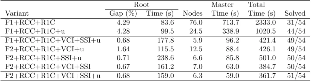
Table 2 gives the comparison of BCP variants. It contains average values for the root gap, geometric mean values for the root solution time, the number of branch-and-bound nodes, the geometric mean of the master problem solution time, the geometric mean of total solution time in seconds, and the number of instances solved within the time limit set to 3 hours. For unsolved instances, the solution time is set to the time limit.
Table 2: Comparison of variants of the BCP algorithm
Root Master Total
Variant Gap (%) Time (s) Nodes Time (s) Time (s) Solved
F1+RCC+R1C 4.29 83.6 76.0 713.7 2333.0 31/54 F1+RCC+R1C+u 4.28 99.5 24.5 338.9 1020.5 44/54 F1+RCC+R1C+VCI+SSI+u 0.68 177.8 5.9 96.2 421.4 49/54 F2+RCC+R1C+VCI+u 1.64 115.5 12.5 88.4 426.1 49/54 F2+RCC+R1C+SSI+u 0.71 238.6 6.6 85.8 501.0 50/54 F2+RCC+R1C+VCI+SSI 0.67 161.2 7.0 63.0 384.7 50/54 F2+RCC+R1C+VCI+SSI+u 0.68 159.0 6.3 59.0 361.7 51/54 We see that the base variant F1+RCC+R1C is the worst as it solves only 31 out of 54 instances. Adding branching on variables uimproves significantly the base variant as variant F1+RCC+R1C+u solves 13 more instances. The best variant F2+RCC+R1C+VCI+SSI+u solves 7 more instances to optimality within the time limit. Table 2 shows that all our contri-butions improve the efficiency of the BCP algorithm. The root gap decreases significantly when new valid inequalities VCI and SSI are separated. Although the root solution time increases when additional inequalities are separated, the overall time decreases due to the much smaller size of the branch-and-bound tree. Thus, branching on variables u has a small effect on the performance of variant F2+RCC+R1C+VCI+SSI+u. However, adding branching on variables uis the simplest way to make the base variant F1+RCC+R1C much more efficient.
If one uses formulation F2 instead of F1, i) the cumulative time to solve the restricted master LP reduces, as the number of variables decreases; ii) the root gap however does not change, as it
is expected from Proposition 1 which shows equivalence of LF1 and LF2; iii) two more instances are solved to optimality; iv) the average reduction of the solution time is relatively small, as the cumulative time to solve the restricted master LP is minor in comparison with the total solution time.
6.3
Comparison with the state-of-the-art algorithm
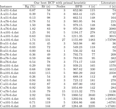
Let us now compare the variants F1+RCC+R1C and F2+RCC+R1C+VCI+SSI+u to the best exact algorithm by Baldacci et al. (2013). For a fair comparison, we do not use initial primal bounds in this experiment. Instead, we rely on the primal heuristic presented in section 5.4 to find feasible solutions. Baldacci et al. (2013) did not set an overall time limit for their algorithm. They set a limit on the number of collections of first-level routes considered, as well as a time limit of 5000 seconds for solving each subproblem with fixed subset of first-level routes. In our BCP algorithm, we set the time limit to 10 hours.
Table 3 shows the summary results of this experiment. For each set of literature instances, we give the average gap between the root dual bound and the best primal bound found (Rg), the geometric mean of the number of branch-and-bound nodes (Nds), the geometric mean of the solution time in seconds (t), and the number of instances solved to optimality (Solved). For a fair comparison, the solution time of (Baldacci et al., 2013) is divided by 1.6 because of the difference in computer speeds. The algorithm in (Baldacci et al., 2013) was tested only on 6 out of 18 instances of set 5. It has not been applied for instances with 10 satellites, as it is based on an enumeration of subsets of first-level routes. Since our algorithms are free from this drawback, they were tested on all instances of set 5.
Table 3: Comparison of two BCP variants with the state-of-the-art exact algorithm for the 2E-CVRP Baldacci et al. (2013)
F1+RCC+R1C F2+RCC+R1C+VCI+SSI+u Literature Set Rg(%) Nds t(s) Solved Rg(%) Nds t(s) Solved t(s) Solved 4A 5.76 14.2 772 51/54 0.91 3.3 144 54/54 271 50/54 4B 4.45 12.7 550 52/54 0.98 3.6 203 54/54 232 52/54 5 5.83 222.9 20612 6/18 1.41 22.5 3215 15/18 8405 3/6 6A 7.04 99.7 2604 24/27 0.89 4.9 233 27/27 802 22/27 6B 3.15 57.8 1562 24/27 0.46 4.3 196 27/27 513 19/27
The base variant F1+RCC+R1C solves to optimality more instances than the best algorithm in the literature. However, the running time of the latter is on average smaller. The variant F2+RCC+R1C+VCI+SSI+u largely outperforms both other algorithms for all sets of instances. Indeed, our best BCP solves to optimality 31 open instances within 10 hours. Detailed results for this variant are given in A. The remaining 3 open instances were solved to optimality by providing the best-known solution of the literature as initial primal bound and using a special parameterisation. Detailed results for these instances are given in B.
Table 4 shows that our BCP algorithm could improve 10 best-known solutions (BKS) for literature instances. Their optimum solution values are given in column Opt. The improvement (Imp) is generally small. Thus, the existing heuristics for the 2E-CVRP have very good quality (at least when applied to literature instances).
6.4
Experimental results for new instances
As all instances from the literature were solved to optimality, we generated a new set of larger instances. The main goal was to test the scalability of our best algorithm, i.e. to determine the size of instances which cannot be solved in a reasonable time.
The new instances involve 5 – 15 satellites and 100 – 300 customers. When testing our algorithm on these instances, we set the time limit to 60 hours. We gave more time to the
Instance BKS Reference Opt Imp (%) Set 5 100-5-1b 1103.55 Amarouche et al. (2018) 1099.35 0.38 100-10-3b 849.73 Amarouche et al. (2018) 848.16 0.19 200-10-1 1538.35 Amarouche et al. (2018) 1537.52 0.05 200-10-1b 1175.81 Amarouche et al. (2018) 1173.07 0.23 200-10-3 1779.68 Amarouche et al. (2018) 1177.49 0.12 200-10-3b 1196.93 Amarouche et al. (2018) 1192.35 0.38 Set 6A C-n101-4 1297.42 Wang et al. (2017) 1292.04 0.41 Set 6B B-n101-4 1500.55 Breunig et al. (2016) 1499.71 0.06 B-n101-5 1395.32 Breunig et al. (2016) 1394.79 0.04 C-n101-5 1964.63 Breunig et al. (2016) 1962.52 0.11 Table 4: Improved best-known solutions for the literature instances
primal heuristic when solving the largest instances. For instances with 300 customers and 10 satellites, this time was set to 600 seconds. For instances with 15 satellites, this time was set to
4· |C|seconds.
Out of 51 instance, our algorithm solved to optimality 23 instances, including some instances with 300 customers or with 15 satellites. The algorithm found both dual and primal bounds for 17 instances. The primal heuristic did not find any feasible solution for 9 instances having 300 customers and/or 15 satellites. Only lower bounds are thus currently known for these instances. We could not obtain dual bounds for 2 instances because the LP solver spent more than one hour to solve the restricted master LP during the first column generation convergence. Detailed results are given in C.
From the results on new instances, we conclude that our algorithm can solve to optimality instances up to 200 customers and 10 satellites, although sometimes in a long run. Our results on new instances up to 200 customers and 10 satellites are consistent with those on literature instances, even if one of these new instances was not solved to optimality. Increasing the instance size to either 300 customers or to 15 satellites makes our algorithm much less efficient. The instances with 300 customers and 15 satellites are particularly challenging, as none of them were solved to optimality.
For the largest instances with 15 satellites, the size of the restricted master problem becomes very large so that its solution takes significant time. In some extreme cases, a modern LP solver cannot solve it within 1 hour. Even when the LP relaxation of the restricted master for large instances can be solved, the primal heuristic based on solving the restricted master is often inefficient. One of the possible remedies is to generate first-level routes dynamically.
7
Conclusions
In this paper we proposed an improved branch-cut-and-price algorithm for the two-echelon ca-pacitated vehicle routing problem. Our BCP algorithm includes both techniques for the classic vehicle routing problems proposed recently and new problem-specific components such as new route based formulation, two families of valid inequalities, and a new branching strategy. The proposed algorithm is empirically shown to be highly efficient, as it solved all instances available in the literature for the 2E-CVRP with up to 200 customers and 10 satellites. 34 instances were solved to optimality for the first time.
In order to inspire further progress on solution approaches for the 2E-CVRP and related problems, a new set of 51 instances is proposed to the community. Among them, 28 instances are currently open. Testing our algorithm on new instances revealed its limitations.
Dynamic generation of first-level routes is essential if one wants to solve instances with more than 15 satellites. Our new formulation for the problem without product flow variables allows one to do such dynamic generation. However, column generation of first-level routes is not
straight-forward for the modified formulation. A first-level route has coefficient one in constraints (12) if and only if it visits at least one satellite in a certain set. Thus, these constraints resemble strong capacity constraints introduced in (Baldacci et al., 2008). They are non-robust (Pessoa et al., 2008), i.e. they modify the structure of the pricing problem for the first level.
Our BCP algorithm could be extended to the two-echelon location-routing problem (Con-tardo et al., 2012) in which satellites have predefined capacities and fixed opening costs. Our preliminary research showed that additional valid inequalities are necessary for this variant of the problem. If one separates only the valid inequalities considered in this paper, the LP relaxation of the route based formulation in general, does not produce strong lower bounds.
Another important possible extension of our algorithm concerns the two-echelon vehicle rout-ing problem with time windows. This problem variant was considered by Dellaert et al. (2019). However, the authors impose there a restrictive assumption that city freighter can receive prod-ucts from only one urban truck. It would be useful to consider the 2E-CVRP with time windows without this assumption.
Acknowledgments
We are grateful to Fran¸cois Vanderbeck whose efforts contributed to obtaining the Ph.D. stu-dentship for the first author. We also want to thank Artur Alves Pessoa who inspired the idea of the modified formulation presented in the paper.
Experiments presented in this paper were carried out using the PlaFRIM (Federative Plat-form for Research in Computer Science and Mathematics), created under the Inria PlaFRIM development action with support from Bordeaux INP, LABRI and IMB and other entities: Conseil R´egional d’Aquitaine, Universit´e de Bordeaux, CNRS and ANR in accordance to the “Programme d’Investissements d’Avenir”.
References
Youcef Amarouche, Rym N. Guibadj, and Aziz Moukrim. A Neighborhood Search and Set Cover Hybrid Heuristic for the Two-Echelon Vehicle Routing Problem. In Ralf Bornd¨orfer and Sabine Storandt, editors, 18th Workshop on Algorithmic Approaches for Transportation Modelling, Optimization, and Systems (ATMOS 2018), volume 65 of OpenAccess Series in Informatics (OASIcs), pages 11:1–11:15, Dagstuhl, Germany, 2018. Schloss Dagstuhl–Leibniz-Zentrum fuer Informatik.
Roberto Baldacci and Aristide Mingozzi. A unified exact method for solving different classes of vehicle routing problems. Mathematical Programming, 120(2):347–380, 2009.
Roberto Baldacci, Nicos Christofides, and Aristide Mingozzi. An exact algorithm for the vehicle routing problem based on the set partitioning formulation with additional cuts. Mathematical Programming, 115:351–385, 2008.
Roberto Baldacci, Aristide Mingozzi, and Roberto Roberti. New route relaxation and pricing strategies for the vehicle routing problem. Operations Research, 59(5):1269–1283, 2011. Roberto Baldacci, Aristide Mingozzi, Roberto Roberti, and Roberto Wolfler Calvo. An exact
algorithm for the two-echelon capacitated vehicle routing problem. Operations Research, 61 (2):298–314, 2013.
J. M. Belenguer, M. C. Martinez, and E. Mota. A lower bound for the split delivery vehicle routing problem. Operations Research, 48(5):801–810, 2000.
Jos´e-Manuel Belenguer, Enrique Benavent, Christian Prins, Caroline Prodhon, and Roberto Wolfler Calvo. A branch-and-cut method for the capacitated location-routing prob-lem. Computers & Operations Research, 38(6):931 – 941, 2011.
U. Breunig, V. Schmid, R.F. Hartl, and T. Vidal. A large neighbourhood based heuristic for two-echelon routing problems. Computers and Operations Research, 76:208 – 225, 2016. Claudio Contardo and Rafael Martinelli. A new exact algorithm for the multi-depot vehicle
routing problem under capacity and route length constraints. Discrete Optimization, 12:129 – 146, 2014.
Claudio Contardo, Vera Hemmelmayr, and Teodor Gabriel Crainic. Lower and upper bounds for the two-echelon capacitated location-routing problem. Computers & Operations Research, 39(12):3185 – 3199, 2012.
Claudio Contardo, Jean-Fran¸cois Cordeau Cordeau, and Bernard Gendron. A computational comparison of flow formulations for the capacitated location-routing problem. Discrete Opti-mization, 10(4):263 – 295, 2013.
Teodor Gabriel Crainic, Nicoletta Ricciardi, and Giovanni Storchi. Models for evaluating and planning city logistics systems. Transportation science, 43(4):432–454, 2009.
Teodor Gabriel Crainic, Guido Perboli, Simona Mancini, and Roberto Tadei. Two-echelon vehicle routing problem: A satellite location analysis. Procedia - Social and Behavioral Sciences, 2 (3):5944 – 5955, 2010.
Teodor Gabriel Crainic, Antonio Sforza, and Claudio Sterle. Location-routing models for two-echelon freight distribution system design. Technical Report 2011-40, CIRRELT, 2011. R. Cuda, G. Guastaroba, and M.G. Speranza. A survey on two-echelon routing problems.
Computers and Operations Research, 55:185 – 199, 2015.
Nico Dellaert, Fardin Dashty Saridarq, Tom Van Woensel, and Teodor Gabriel Crainic. Branch and price based algorithms for the two-echelon vehicle routing problem with time windows. Transportation Science, In Press, 2019.
I. Dunning, J. Huchette, and M. Lubin. JuMP: A modeling language for mathematical opti-mization. SIAM Review, 59(2):295–320, 2017.
Jesus Gonzalez-Feliu, Guido Perboli, Roberto Tadei, and Daniele Vigo. The two-echelon capac-itated vehicle routing problem. Technical Report DEIS OR.INGCE 2007/2, Department of Electronics, Computer Science, and Systems, University of Bologna,, 2007.
Vera C. Hemmelmayr, Jean-Fran¸cois Cordeau, and Teodor Gabriel Crainic. An adaptive large neighborhood search heuristic for two-echelon vehicle routing problems arising in city logistics. Computers & Operations Research, 39(12):3215 – 3228, 2012.
Mads Jepsen, Bjorn Petersen, Simon Spoorendonk, and David Pisinger. Subset-row inequalities applied to the vehicle-routing problem with time windows. Operations Research, 56(2):497– 511, 2008.
Mads Jepsen, Simon Spoorendonk, and Stefan Ropke. A branch-and-cut algorithm for the symmetric two-echelon capacitated vehicle routing problem. Transportation Science, 47(1): 23–37, 2013.
G. Laporte and Y. Nobert. A branch and bound algorithm for the capacitated vehicle routing problem. Operations-Research-Spektrum, 5(2):77–85, Jun 1983.
Adam N. Letchford and Juan-Jos´e Salazar-Gonz´alez. Projection results for vehicle routing. Mathematical Programming, 105(2):251–274, Feb 2006.
Jens Lysgaard. CVRPSEP: a package of separation routines for the capacitated vehi-cle routing problem, 2018. URL http://econ.au.dk/research/researcher-websites/ jens-lysgaard/cvrpsep/.
Jens Lysgaard, Adam N. Letchford, and Richard W. Eglese. A new branch-and-cut algorithm for the capacitated vehicle routing problem. Mathematical Programming, 100(2):423–445, Jun 2004.
Diego Pecin, Artur Pessoa, Marcus Poggi, and Eduardo Uchoa. Improved branch-cut-and-price for capacitated vehicle routing.Mathematical Programming Computation, 9(1):61–100, 2017a. Diego Pecin, Artur Pessoa, Marcus Poggi, Eduardo Uchoa, and Haroldo Santos. Limited memory rank-1 cuts for vehicle routing problems. Operations Research Letters, 45(3):206 – 209, 2017b. Guido Perboli, Roberto Tadei, and Daniele Vigo. The two-echelon capacitated vehicle routing
problem: Models and math-based heuristics. Transportation Science, 45(3):364–380, 2011. Artur Pessoa, Marcus Poggi de Arag˜ao, Marcus, and Eduardo Uchoa. Robust
branch-cut-and-price algorithms for vehicle routing problems. In Bruce Golden, S. Raghavan, and Edward Wasil, editors,The Vehicle Routing Problem: Latest Advances and New Challenges, volume 43 ofOperations Research/Computer Science Interfaces, pages 297–325. Springer US, 2008. Artur Pessoa, Eduardo Uchoa, and Marcus Poggi de Arag˜ao. A robust branch-cut-and-price
algorithm for the heterogeneous fleet vehicle routing problem. Networks, 54(4):167–177, 2009. Artur Pessoa, Ruslan Sadykov, Eduardo Uchoa, and Fran¸cois Vanderbeck. Automation and combination of linear-programming based stabilization techniques in column generation. IN-FORMS Journal on Computing, 30(2):339–360, 2018.
Artur Pessoa, Ruslan Sadykov, Eduardo Uchoa, and Fran¸cois Vanderbeck. A generic exact solver for vehicle routing and related problems. In Andrea Lodi and Viswanath Nagarajan, editors,Integer Programming and Combinatorial Optimization, volume 11480 ofLecture Notes in Computer Science, pages 354–369, Cham, 2019. Springer International Publishing.
Edward Rothberg. An evolutionary algorithm for polishing mixed integer programming solutions. INFORMS Journal on Computing, 19(4):534–541, 2007.
Ruslan Sadykov, Eduardo Uchoa, and Artur Pessoa. A bucket graph based labeling algorithm with application to vehicle routing. Cadernos do LOGIS 7, Universidade Federal Fluminense, October 2017.
Ruslan Sadykov, Fran¸cois Vanderbeck, Artur Pessoa, Issam Tahiri, and Eduardo Uchoa. Pri-mal heuristics for branch-and-price: the assets of diving methods. INFORMS Journal on Computing, In Press, 2018.
Fernando Afonso Santos, Geraldo Robson Mateus, and Alexandre Salles da Cunha. A branch-and-cut-and-price algorithm for the two-echelon capacitated vehicle routing problem. Trans-portation Science, 49(2):355–368, 2015.
Michael Schneider and Maximilian L¨offler. Large composite neighborhoods for the capacitated location-routing problem. Transportation Science, 53(1):301–318, 2019.
Eiichi Taniguchi and Russell G Thompson. Modeling city logistics. Transportation research record, 1790(1):45–51, 2002.
Fran¸cois Vanderbeck, Ruslan Sadykov, and Issam Tahiri. BaPCod — a generic Branch-And-Price Code, 2019. URLhttps://realopt.bordeaux.inria.fr/?page_id=2.
Kangzhou Wang, Yeming Shao, and Weihua Zhou. Matheuristic for a two-echelon capacitated vehicle routing problem with environmental considerations in city logistics service. Trans-portation Research Part D: Transport and Environment, 57:262 – 276, 2017.
Zheng-Yang Zeng, Wei-Sheng Xu, Zhi-Yu Xu, and Wei-Hui Shao. A hybrid GRASP+VND heuristic for the two-echelon vehicle routing problem arising in city logistics,. Mathematical Problems in Engineering, pages 1–11, 2014.
A
Detailed BCP results for literature instances
In following tables, Rg stands for the root gap, Rt stands for the time spent in the root node, BPB is the best primal bound found, and t stands for the total time spent. Note that if the time in the column “Literature” has prefix “>” for a given instance, Baldacci et al. (2013) did not solve this instance to optimality.
In sets 4A and 4B, instances Instance50-i.dat with i = 1,2. . .18 have two satellites. Instances with i = 19,20. . .36 have three satellites. Instances with i = 37,38. . .54 have five satellites. In set 5, instance names have the format 2eVRP_i_j_k.dat with i the number of customers, j the number of satellites, and k an identifier. In sets 6A and 6B, instance names have the formI-ni-j.datwith an identifierI that is the letter A, B or C,i−1 the number of customers, andj the number of satellites.
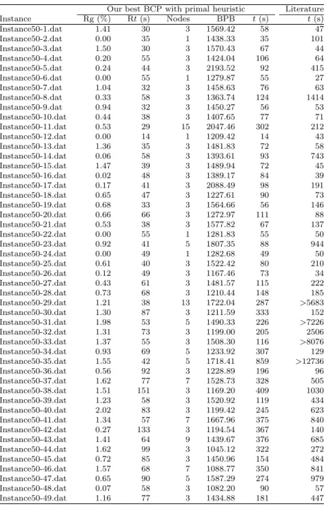
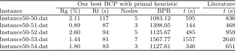
Table 5: Results of experiments on instances of set 4A
Our best BCP with primal heuristic Literature Instance Rg (%) Rt(s) Nodes BPB t(s) t(s) Instance50-1.dat 1.41 30 3 1569.42 58 47 Instance50-2.dat 0.00 35 1 1438.33 35 101 Instance50-3.dat 1.50 30 3 1570.43 67 44 Instance50-4.dat 0.20 55 3 1424.04 106 64 Instance50-5.dat 0.24 44 3 2193.52 92 415 Instance50-6.dat 0.00 55 1 1279.87 55 27 Instance50-7.dat 1.04 32 3 1458.63 76 63 Instance50-8.dat 0.33 58 3 1363.74 124 1414 Instance50-9.dat 0.94 32 3 1450.27 56 53 Instance50-10.dat 0.44 38 3 1407.65 77 71 Instance50-11.dat 0.53 29 15 2047.46 302 212 Instance50-12.dat 0.00 14 1 1209.42 14 43 Instance50-13.dat 1.36 35 3 1481.83 72 58 Instance50-14.dat 0.06 58 3 1393.61 93 743 Instance50-15.dat 1.47 39 3 1489.94 72 45 Instance50-16.dat 0.02 48 3 1389.17 84 39 Instance50-17.dat 0.17 41 3 2088.49 98 191 Instance50-18.dat 0.65 47 3 1227.61 90 73 Instance50-19.dat 0.68 33 3 1564.66 56 146 Instance50-20.dat 0.66 66 3 1272.97 111 88 Instance50-21.dat 0.53 38 3 1577.82 67 137 Instance50-22.dat 0.00 55 1 1281.83 55 50 Instance50-23.dat 0.92 41 5 1807.35 88 944 Instance50-24.dat 0.00 49 1 1282.68 49 50 Instance50-25.dat 0.61 40 3 1522.42 80 210 Instance50-26.dat 0.12 49 3 1167.46 73 34 Instance50-27.dat 0.43 61 3 1481.57 115 222 Instance50-28.dat 0.73 68 3 1210.44 148 185 Instance50-29.dat 1.21 38 13 1722.04 287 >5683 Instance50-30.dat 1.30 87 3 1211.59 333 152 Instance50-31.dat 1.98 53 5 1490.33 226 >7226 Instance50-32.dat 1.31 73 3 1199.00 205 2506 Instance50-33.dat 1.37 55 3 1508.30 116 >8076 Instance50-34.dat 0.93 69 5 1233.92 307 129 Instance50-35.dat 1.55 42 5 1718.41 859 >12736 Instance50-36.dat 0.56 92 3 1228.89 196 96 Instance50-37.dat 1.62 77 7 1528.73 328 505 Instance50-38.dat 1.51 151 3 1169.20 409 1030 Instance50-39.dat 1.23 58 3 1520.92 119 434 Instance50-40.dat 2.02 83 3 1199.42 245 623 Instance50-41.dat 1.34 57 7 1667.96 375 840 Instance50-42.dat 0.27 133 3 1194.54 367 140 Instance50-43.dat 1.41 64 9 1439.67 376 685 Instance50-44.dat 1.62 99 3 1045.12 322 272 Instance50-45.dat 0.72 85 3 1450.96 154 484 Instance50-46.dat 1.57 68 7 1088.77 350 841 Instance50-47.dat 0.65 90 5 1587.29 274 979 Instance50-48.dat 0.07 58 3 1082.20 90 57 Instance50-49.dat 1.16 77 3 1434.88 181 447