MSI Working paper

MSI_1608

Thanks, but no thanks:

Companies’ response to R&D tax credits

Thanks, but no thanks:

Companies’ Response to R&D tax Credits

June 2016

Daniel Neicuǂ Stijn Kelchtermans Peter Teirlinck

ǂ _{Department of Managerial Economics and Innovation, KU Leuven, Belgium}

_{Department of Strategy, Innovation & Entrepreneurship, KU Leuven, Belgium}

Abstract

This paper starts from the observation that the majority of firms in Belgium that were eligible for a newly introduced R&D tax credit system does not use it, or is slow to adopt, despite significant potential cost savings. We hypothesize that the R&D support landscape is complex for firms to navigate and that they may cope by relying on their peers’ behaviour to inform their own adoption decisions. We identify endogenous peer effects in industry- and location-based peer groups by exploiting the intransitivity in firms’ peer group networks as well the variation in peer group sizes. The results show that firms’ decisions to use R&D tax credits are indeed influenced by the choices of their peers, primarily in the time window following the introduction. Our analysis complements the literature on peer effects in firm decision making and suggests improvements for the communication of new public support measures for business R&D.

Keywords: R&D tax credits, peer effects, information diffusion, social interactions.

1. Introduction

Social, or ‘peer-to-peer’, interactions have been considered in the literature as a way to transfer knowledge (Noorderhaven & Harzing, 2009; Corredoira & Rosenkopf, 2010). In particular, economic agents may draw lessons and create expectations from the observation of actions and outcomes experienced by others (Manski, 2000). Through this lens, peer effects have been studied extensively for explaining social behaviour, such as job-searching (Nanda and Sørensen, 2010; Cappellari and Tatsiramos, 2011) or the initiation of sexual activity (Card and Giuliano, 2011). The social connectedness of firm decision-making has been investigated less, arguably due to the difficulty in directly observing inter-company interaction, which we address in section 2. Nevertheless, this social dimension is a key issue in studying adoption decisions, that is, its comprehensive assessment necessitates rising above the level of the individual firm to include social feedback effects (Hall, 2004). Despite the empirical challenges in observing peer groups, a number of studies have looked into the role of ‘social influence’ in the corporate world by considering, in various settings, whether a larger number of adopters of a certain decision increases the probability of it spreading further. Evidence of such imitation behaviour has been provided in studies of market entry (Gort & Konakayama, 1982; Kennedy, 2002; Lu, 2002; Debruyne & Reibstein, 2005), investment banking (Haunschild & Miner, 1997) and corporate financial policy (Leary & Roberts, 2014).

Our paper complements the literature on peer effects in firm decision making by studying the adoption of R&D support. The theoretical basis for our analysis is that peer effects may play a role if the R&D support landscape is complex and firms may rely on their peers’ decisions as an input in their own adoption decisions. In Belgium, the setting we study, one would at first sight expect rapid and widespread adoption, with little role for peer effects. Reasons include the fact that the administrative cost of applying for the tax credit is essentially zero and that the tax credit is effectively implemented as a wage subsidy for R&D workers, so a firm needn’t

report positive profits to benefit from the measure. In other words, not using the R&D tax credit while being eligible comes down to leaving money on the table. However, audits of the portfolio of R&D support mechanisms have found it to resemble a ‘thicket’ that firms find difficult to navigate, up to the point where many eligible firms do not use support they are entitled to (Soete, 2012).2 Dumont (2013), reporting descriptive evidence on the uptake of the

2 _{The so-called “Soete reports” (Soete, 2012) considered R&D support in the Flemish region, which is the largest}

of the three regions in Belgium). However, the R&D support landscape in the Walloon and Brussels Capital Region is also characterized by a proliferation of support measures.

3

fiscal incentives for R&D introduced in Belgium in 2005, concludes that most R&D active companies do not use the measure four years after its introduction. Our sample of Belgian firms shows that even by 2011, hardly 40% of the firms eligible for the tax credit use it. Similar evidence has been reported for other countries. For example, Falk et al. (2009) find that companies in Austria lack awareness of the structure of tax incentives and point towards insufficient information as a reason for non-adoption. A study by Bozio et al. (2014) reveals that in France, after the shift from an incremental to a more generous volume-based tax credit scheme in 2008, the share of eligible firms that does not apply still surpasses one in three companies.

The situation in which initially only a relatively small share of eligible firms adopts the tax credit in a complex support environment creates the opportunity for peer effects to occur. More specifically, if information about support is complex – i.e. the abundance of support schemes – and uncertain – in terms of eligibility – firms may resort to heuristics in their decision making. One such approach is to imitate decisions of peers who have adopted the measure earlier. Prior work has found evidence of peer effects in firm decision making in diverse areas, including financial decisions (Leary & Roberts, 2014), marketing choices (Debruyne & Reibstein, 2005) and compensation of top management (Albuquerque, 2009).

Using the peer effects rationale, we investigate to what extent firms’ adoption of the R&D tax credit can be attributed to decisions of their peers, rather than own firm characteristics or unobserved shocks pushing whole groups of companies towards adoption of the tax credit. Analysing a sample of 1,981 R&D active companies in Belgium, and relying on an innovative – in this setting – IV approach for identifying the endogenous peer effects, we find that a firm’s decision to take up R&D tax credits is influenced by the choices of peers. We start from the empirical observation that a majority of possible users of R&D tax credits seem reluctant to use them, despite the significant wage cost reduction involved. Attributing low adoption rates to lack of information, this paper is the first to demonstrate how peer effects shape firms’ response to R&D public support schemes with limited information regarding peer networks. Our findings show that imitation is one of the strategies employed by firms in order to cope with the multitude of public support measures they face.

Our paper makes the following contributions. First, we complement the literature on support for innovation by showing how peer effects influence firms’ usage of public support schemes. This is important, as an accurate understanding of the dynamics of firm choices is essential for

4

reducing inefficiencies, i.e. the belated absorption of public support for R&D. Our results suggest that firms develop strategies to cope with the complexity of the R&D support landscape by imitating firms who adopt earlier. The finding that imitation occurs in peer groups that follow industry- and distance-based default lines suggests possible policy interventions for reducing inefficiencies in usage of R&D support. More specifically, adoption by eligible firms could be expedited by communicating the measure to sufficiently fine-grained sectors and in a geographical distributed way. As opposed to broad policy communications, ‘narrowcasting’ would help to reach many localized firm clusters, or peer groups, allowing for rapid peer-to-peer influence, once initial adoption has taken place. Second, the establishment of peer-to-peer effects as a significant factor driving firms’ selection into support schemes informs the methodological literature on selection bias in program evaluation (Imbens & Wooldridge, 2009). Namely, the existence of peer effects calls for looking beyond the individual firm to explain selection into support programs. More generally, by using recent advances in identification strategy for peer effects (Bramoullé et al., 2009; De Giorgi et al., 2010), this paper contributes to the broader literature on peer effects between firms. More specifically, by relying on a ‘nearest neighbours’ peer group definition, peer groups vary at the individual firm level. This variation implies the presence of ‘excluded peers’ i.e. firms who are not part of firm i’s peer group, but who are

peers of i’s peers. The exogenous characteristics of these excluded peers act as instruments for

the endogenous peer effect because they are correlated with the adoption decision of firm i’s

peers by means of social interactions, but they are uncorrelated with shocks affecting firm i

and its peer group. Given the high degree of clustering in many ‘small world’ firm networks (e.g. Fleming & Marx, 2006), this approach of exploiting intransitivity in firms’ networks is more generally applicable to identify peer effects in other settings. One example would be the analysis of knowledge spillovers in networks of inventive activity, as measured by co-patenting between firms.

The rest of the paper is organized as follows. Section 2 presents the definition of peer groups, which ties into our identification strategy and empirical model, both of which are discussed in section 3. Section 4 discusses the results of the analysis of peer effects in R&D tax credit adoption and reports the robustness checks. Section 5 concludes.

2. Peer Group Definition

Any identification of peer effects in firm decision making needs to start from the definition of peer groups. This constitutes a key challenge since the circles of peers in which information is

5

transferred may be informal and therefore hard to trace empirically. While some settings in the social interaction literature provide an institutional dimension that provides a handle on peer groups, e.g. class allocations of students, it is not straightforward what firms jointly constitute a peer group. In order to deal with the lack of precise information on peer groups, we draw on literature that has studied firm interactions to identify the defining characteristics of firms’ peer groups. In particular, we take industry and geographical location as the determinants of a firm’s network, following the long-standing observation in the economic geography literature that economic activity tends to be clustered in relatively small geographic areas (e.g. Marshall, 1920; Krugman, 1991). The intersection of industry and geography therefore provides an intuitive perspective on peer groups. Further, Porter (1990) argued that innovation dynamics in clusters are stimulated by local competition and peer pressure among firms. These firm efforts and the associated influencing of peers needn’t be restricted to innovation in a narrow sense, but may well extend to all innovation-enabling activities, such as accessing public R&D support. A more general motivation to include the industry dimension in the construction of peer groups is homophily, which is considered an important determinant for social network formation, with actors more likely to connect to, or be influenced by, others who resemble themselves in one or more dimensions (Boschma & Frenken, 2010). Empirical work has found industry to be a defining feature of the context where different types of inter-firm influencing take place. For example, the revision of a company's previous financial statements has been found to induce share price declines not only for the focal firm, but also among non-restating firms in the same industry (Gleason et al., 2008). Graham & Harvey (2001) showed that the financing decisions by peer firms in the same industry, in particular competitors, influence the focal firm’s own decisions. Measuring firms’ industry membership at 3-digit SIC level, Leary and Roberts (2014) show how within-industry peers are a more important determinant of firms’ financial policies, such as their leverage ratio, than changes in firm-specific characteristics. Besides industry, geographical proximity is also prominent in the social interactions literature since short distances favour contacts and facilitate knowledge exchange (e.g. Bell & Song, 2007; Nam, Manchanda, & Chintagunta, 2007). Several empirical studies have shown the geographically bounded nature of (technological) knowledge spillovers (e.g. Jaffe et al., 1993; Almeida & Kogut, 1999; Audretsch & Feldman, 1996; Fritsch & Franke, 2004). Further, geographical proximity correlates positively with other dimensions of proximity, such as social and cognitive proximity (Boschma, 2005), and therefore partially captures other linkages with

6

peers, such as social relations between employees or being embedded in the same knowledge community.

Based on these insights from previous work on firm interactions and knowledge spillovers, we define peer groups using a nearest neighbour logic. More specifically, we take as a firm’s peers the K closest firms (KNN) within the same 3-digit NACE sector.3 _{This definition allows for}

intransitivity in the network of firms i.e. the peers of the focal firm’s peers are not necessarily peers of the focal firm itself. We will exploit this feature in order to identify peer effects, as explained in section 3.

As a first ‘rough’ check on the potential role of distance in peer influence, we relate firms’ usage of R&D tax credits to geographical location4. We see that use of R&D tax credits is not spread uniformly, but rather that locations with higher shares of tax credit users tend to be clustered. Note that firms may be considered randomly allocated to a location with respect to their usage of the R&D tax credit. In other words, it is unlikely that firms would co-locate for reasons that drive their decision to use R&D tax credits. The analysis will control for other R&D-related factors that may explain co-location of firms, such as R&D intensity.

Finally, we note that it is common for empirical work using social network data to observe only a sample of all nodes in the network. Our work is no exception: the data we use for the peer group definition and the estimation is a sample of R&D tax credit users, namely those firms for which characteristics from the business R&D survey are available.5 Using a sample of the population would imply measurement error if there are firms in the population that are not part of the sample but that are in the (true) peer groups of sampled firms. It is important for our approach that firms were not selected into the sample based on location, making it a reasonable assumption that missing links in peer groups are random.6 _{However, even in the}

case of fully random sampling, networks can still be misspecified (Chandrasekhar & Lewis, 2011). While the definition of peer groups draws on prior evidence and is informed by the patterns shown in the descriptive statistics, the lack of direct observation of peer groups and

3 _{The peer groups we consider are geographically confined to Belgium, which we deem reasonable since R&D}

tax credits are granted by the Belgian federal authority, and firms within Belgium therefore constitute the relevant firm network.

4 _{Technically, we observe a firm’s location by a NIS-code, which denotes a statistical unit that corresponds to}

municipalities. The median size of a municipality is 40.1 km², with a standard deviation of 37.7 km². The average number of firms per municipality is 3.18, with a standard deviation of 4.23.

5 _{Note that firms are not selected into the sample based on the dependent variable, as we observe both users and}

non-users of the R&D tax credit.

6 _{Since the importance of R&D tends to be strongly related to the type of industry, which is the other dimension}

in our peer group definition, firms in a given industry are likely to be treated similarly with respect to inclusion in the business R&D survey, and thus our sample.

7

the sampling still allow for measurement error and thus a misspecified network structure. Two remarks are in order here. First, virtually all studies of peer effects suffer from potential measurement error in the definition of peer groups, since it is typically not known what the precise mechanism is that underlies the interaction, the type and degree of interaction being specific to the empirical context (De Giorgi et al., 2010). In our analysis of the adoption of public support for R&D, peer effects may arise due to imitation of other firms’ decisions,

without the need for close interaction. This alleviates concerns about not observing explicit collaborations between firms, and even makes such information unnecessary. More generally, empirical work shows a broad range of peer group definitions, ranging from very comprehensive, e.g. the effect on consumption by peers of the same race in the same state of residence in the U.S. (Charles, Hurst, & Roussanov, 2009) to highly restrictive, e.g. the effect on student performance by roommates in the same college dorm (Sacerdote, 2001). Our definition is rather comprehensive, which is consistent with the setting under consideration, where any influence by peers on the focal firm’s decision to adopt the R&D tax credit merely requiring observation of peers’ behaviour, rather than explicit interaction.

Second, we adopt a conservative approach regarding the specification of peer groups and conduct a series of robustness checks in section 4.6 to ascertain that any identified peer influence is not conditional on a given measurement of peer groups. First, we apply a network randomization test, in which we scramble the peer groups by reshuffling the sample firms across locations and industries, and then re-estimate the model to verify that the results on peer effects are not obtained when considering any random peer group network.Second, we check the sensitivity of results for different choices of peer group size (K). Third, we define peer groups at different industry aggregation levels and include additional industry and regional controls in the model.

3. Identification Strategy & Model

The identification of peer effects is notoriously challenging, as originally explained by Manski (1993). In this section, we explain the two key identification problems and how we exploit intransitivity in the firm network, i.e. partially overlapping peer groups, to address them (Bramoullé et al., 2009; De Giorgi et al., 2010). The first problem, referred to as reflection, essentially means that it is hard to disentangle whether a firm’s decision to use the R&D tax credit system causes its peer to do the same, or whether it does so as a consequence of its peers’ actions. In other words, the setting of peer effects suffers from a simultaneity problem. The second problem in identifying peer effects consists of endogeneity issues due to endogenous

8

peer group formation and unobserved correlated shocks. Both of these factors may cause the decisions of an individual firm and its peer group to be correlated, confounding any true peer effects. Common unobserved shocks refer to factors that cause both the focal firm and its peer group to adopt the and R&D tax credit, without any peer influence taking place. In our setting this would occur if, for example, the focal firm and its peers rely on the same accountant, alerting all its clients of the introduction of the R&D tax credit system.

Following De Giorgi, Pellizzari, & Redaelli (2010), we now provide a more detailed discussion of the identification challenges and the approach we take to address them. Consider the following linear-in-means spatial7 model, omitting time subscripts for simplicity:

𝑦_𝑖 = 𝛼 + 𝛽𝐸(𝑦|𝐺_𝑖) + 𝛾𝐸(𝑥|𝐺_𝑖) + 𝛿𝑥_𝑖+ 𝑢_𝑖 (1)

The dependent variable 𝑦_𝑖 indicates whether firm 𝑖 has adopted the R&D tax credit8_{, 𝑥}

𝑖 are firm characteristics, 𝐸(𝑦|𝐺_𝑖) is the average choice of firms in 𝑖’s peer group, which is denoted by 𝐺_𝑖. 𝐸(𝑥|𝐺_𝑖) are the average characteristics of firm 𝑖’s peers. Practically, a firm’s peers are indicated through the use of a spatial weighting matrix 𝑊, which implements the peer group definition such that 𝑊𝑦 = 𝐸(𝑦|𝐺_𝑖) and 𝑊𝑥 = 𝐸(𝑥|𝐺_𝑖). Parameter 𝛽 captures the endogenous effect i.e. ‘true’ peer effect, and 𝛾 the exogenous effect, sometimes also referred to as the

contextual effect (Manski, 1993).

We focus first on the reflection problem and assume for now the absence of any endogeneity concerns i.e. 𝐸(𝑢𝑖|𝐺𝑖, 𝑥𝑖) = 0. As mentioned before, our identification approach hinges on the fact that peer groups are only partially overlapping. To understand this, first consider the case where peer groups overlap perfectly such that, if firm 𝑖 and firm 𝑗 are in the same peer group, their peer groups coincide i.e. 𝐺_𝑖 = 𝐺_𝑗. As Manski (1993) already argued, in this case the endogenous effect 𝛽 cannot be identified separately from exogenous effect 𝛾.9 A less ambitious approach is therefore to simply estimate a single parameter for the combination of

7 _{The label ‘spatial’ is due to the fact that the modelled interactions are determined by firms’ locations.}

8 _{Note that although our dependent variable (adoption of the R&D tax credit) is binary, we stick to the approach}

taken by De Giorgi, Pellizzari, & Redaelli (2010), who study the binary choice of major in higher education. They also opt for a linear model, which allows for a clearer exposition of the identification strategy. Some work has been done on identifying peer effects in binary choice models, exploiting non-linearity to separate endogenous from exogenous effects (Brock & Durlauf, 2007). However, current implementations in statistical software ignore the existence of correlated effects – i.e. spatially correlated errors – due to strict multivariate distributional assumptions needed to identify the model. We consider that accounting for unobserved peer group characteristics that may drive firms’ adoption decision to be paramount to properly identifying the endogenous peer effect, and we thus choose to estimate a (spatial) linear probability model.

9 _{Taking the average of equation (1) over group 𝐺}

𝑖 shows that 𝐸(𝑦|𝐺𝑖) is a linear combination of the other

9

endogenous and exogenous effects without separating them.10 However, in our empirical framework, the KNN-based peer groups are not fixed across firms, hence 𝐸(𝑦|𝐺_𝑖) varies within peer groups. Consider the following simple example to illustrate how this features achieves identification in the face of the reflection problem. Say firms A, B and C are part of the same industry, which also contains other firms. Firms A and B are nearest neighbours (with

𝐾 = 3) and thus part of the same peer group, based on industry and distance. Firm B and C are also nearest neighbors, but, given the geographical distribution of firms in the industry, firms A and C are not (see Figure 1). This layout results in ‘excluded peers’ i.e. firms who are not in the focal firm’s peer group but who are part of the groups of its peers. Firm A is excluded from the peer group of firm C, and vice versa, while B’s peer group includes both A and C.

Figure 1: Example layout of peer groups

More formally, rewrite equation (1) by taking averages over peer groups, allowing them to vary by firm 𝑖:

𝐸(𝑦_𝑖|𝐺_𝑖) = 𝛼 + 𝛽𝐸[𝐸(𝑦|𝐺𝑗)|𝐺𝑖] + 𝛾𝐸[𝐸(𝑥|𝐺𝑗)|𝐺𝑖] + 𝛿𝐸(𝑥𝑖|𝐺𝑖) (2)

with 𝑗 a member of 𝑖’s peer group, and 𝐺_𝑗 never identical to 𝐺_𝑖.11 With respect to the preceding example we can write, omitting firms other than 𝐴, 𝐵 or 𝐶: 𝐺𝐴 = {𝐵}, 𝐺𝐵 = {𝐴, 𝐶}, 𝐺𝐶 =

{𝐵}. Equation (1) can then be written for the three firms as follows:

𝑦_𝐴 = 𝛼 + 𝛽𝑦_𝐵+ 𝛾𝑥_𝐵+ 𝛿𝑥_𝐴 + 𝑢_𝐴𝐴 𝑦𝐵 = 𝛼 + 𝛽 ( 𝑦_𝐴+ 𝑦_𝐶 2 ) + 𝛾 ( 𝑥_𝐴+ 𝑥_𝐶 2 ) + 𝛿𝑥𝐵+ 𝑢𝐵𝐵 𝑦𝐶 = 𝛼 + 𝛽𝑦𝐵+ 𝛾𝑥𝐵+ 𝛿𝑥𝐶+ 𝑢𝐶𝐶

To see how we achieve identification, consider the reduced form equations:

10 _{Typically, the absence of either endogenous peer effects (e.g. Brooks-Gunn et al., 1993) or contextual peer}

effects (e.g. Klier & McMillen, 2008) is assumed.

11 _{As we explain below, our choice of the number of nearest neighbours allows for partially overlapping peer}

groups.

A

B

10 𝑦𝐴 = (𝛼 + 𝛼𝛽(1 + 𝛽) 1 − 𝛽² ) + (𝛽(𝛾 + 𝛿) 1 − 𝛽² + 𝛾) 𝑥𝐵+ ( 𝛽(𝛾 + 𝛿𝛽) 1 − 𝛽² ) ( 𝑥𝐴 + 𝑥𝐶 2 ) + 𝛿𝑥𝐴+ 𝜎𝐴𝐴 𝑦𝐵= ( 𝛼(1 + 𝛽) 1 − 𝛽² ) + ( 𝛾 + 𝛿 1 − 𝛽²) 𝑥𝐵+ ( 𝛾 + 𝛿𝛽 1 − 𝛽²) ( 𝑥𝐴+ 𝑥𝐶 2 ) + 𝜎𝐵𝐵 𝑦𝐶 = (𝛼 + 𝛼𝛽(1 + 𝛽) 1 − 𝛽² ) + (𝛽(𝛾 + 𝛿) 1 − 𝛽² + 𝛾) 𝑥𝐵+ ( 𝛽(𝛾 + 𝛿𝛽) 1 − 𝛽² ) ( 𝑥_𝐴 + 𝑥_𝐶 2 ) + 𝛿𝑥𝐶+ 𝜎𝐶𝐶

where the reduced form error terms 𝜎_𝐴𝐴, 𝜎_𝐵𝐵 and 𝜎_𝐶𝐶 are linear combinations of the structural error terms 𝑢_𝐴𝐴, 𝑢_𝐵𝐵 and 𝑢_𝐶𝐶. The four structural parameters are identified from the four reduced form parameters.12 Note that our identification approach relies on the assumption that – referring to the example – excluded peer firm C does not influence firm A directly. As argued in the section on peer group definition, it seems reasonable to assume that distant firms, in terms of both geographical distance and type of industry, only exert an indirect influence. The second main identification problem concerns endogeneity due to self-selection of firms into peer groups or the presence of unobserved group-level shocks. Formally, the error term may be written as:

𝑢_𝑖𝑔 = 𝜇𝑖+ 𝜃𝑔+ 𝜖𝑖

with 𝑔 denoting the peer group (𝐴, 𝐵 or 𝐶 in the preceding example), 𝜇𝑖 an individual fixed effect, and 𝜃𝑔 a group fixed effect (e.g. the aforementioned ‘common accountant’ effect13) and

𝜖𝑖 is independently identically distributed random error.

In our setting, firms’ peer group membership is determined by their location and industry. It is unlikely that firms sort into these peer groups in a way that correlates with their subsequent R&D tax credit usage, making 𝜇𝑖 negligible or zero.14 The more serious concern leading to endogeneity, is the existence of unobserved correlated effects at the group level, 𝜃𝑔. It turns out the mechanism of excluded peers serves a double purpose. While it deals with the reflection problem in the absence of endogeneity - as discussed above - it also supplies valid instruments

12 _{In this example, the third equation is redundant, which reflects the fact that only observations with distinct}

groups of peers contribute to identification.

13 _{Another example would be the case of several biotech spin-off companies co-locating in the science park of}

their university and where the involved scientists learn about R&D tax credits through the TTO or a scientific entrepreneurship program run by the university.

14 _{In other studies of peer effects this tends to be a more severe issue, e.g. when analysing students’ choice of}

11

for endogenous peer effects. Consider firm 𝑖’s excluded peers i.e. the firms who are excluded from 𝑖’s peer group but who are included in the group of one or more of 𝑖’s peers. Their characteristics 𝑥 are by design uncorrelated with the group fixed effect of focal firm 𝑖, but are correlated with the mean adoption decision of 𝑖’s group through peer interactions. In terms of the earlier example, 𝑥_𝐶 is a valid instrument for 𝑦_𝐵 in group 𝐴 because 𝑥_𝐶 - which is uncorrelated with 𝜃𝐴 since 𝐶 is not a peer of 𝐴 - affects 𝑦_𝐶 and the latter affects 𝑦_𝐵 through endogenous effects since 𝐶 is a peer of 𝐵. In our sample, the excluded peers for a firm 𝑖 include all firms not among the K nearest neighbors in the industry as the focal firm. Table 1 shows the characteristics of peer groups in our sample for different years and values of 𝐾, in particular the share of firms that have at least 𝐾 nearest neighbors in their industry. These are the firms for which the aforementioned identification strategy based on excluded peers is empirically feasible in our sample. For 𝐾 = 10, we still have a majority of firms for which peer groups do not encompass all firms at the 3-digit NACE industry code level, and therefore serves as the empirical upper bound for 𝐾. For firms with less than 𝐾 nearest neighbors in their industry, the intransitivity principle cannot be used to identify endogenous peer effects because there are no excluded peers to instrument peer choice and characteristics. However, Lee (2007) and Bramoullé, Djebbari, & Fortin (2009) have shown that peer effects are identified if at least two peer groups have different sizes. In this case, the effect of a firm’s characteristics xion its own decision yi can be split into the direct effect and an indirect one, through feedback effects – xA affects yB, which in turn affects yA, assuming A and B are peers. This indirect effect is decreases with group size, which is a term of the denominator of the reduced-form coefficient of xi (Bramoullé et al., 2009). Jointly, intransitivity and variation in group sizes are two network properties that ensure identification. Thus, we set 𝐾 = 10 , which effectively acts as an upper bound on the number of peers, and instrument the endogenous peer effect 𝑊𝑦 by 𝑊𝑥 and, using information of excluded peers, 𝑊𝑋².15 For firms with less than 10 peers, identification comes from variation in peer group sizes. For the remainder of the paper, we stick to the 3-digit NACE industry level and 10 nearest neighbours as the main peer group definition.

12

Table 1 Percentage of firms having at least K nearest neighbours in their 3-digit NACE industry

K 2007 2009 2011 2 89% 94% 92% 3 80% 87% 87% 4 75% 83% 80% 5 65% 78% 75% 6 63% 69% 69% 7 60% 65% 67% 8 57% 64% 65% 9 56% 60% 62% 10 54% 55% 58%

To estimate the model in (1), we use Kelejian & Prucha’s (2010) spatial IV estimator, which is implemented in the R package sphet (Piras, 2010). The estimator permits spatial correlation between the error terms i.e. they are modelled as:16

𝑢_𝑖 = 𝜃𝑀𝑢 + 𝜖_𝑖. (3)

The resulting SARAR model is fairly general in its specification17 and has been used in prior work that estimates spatial peer effects, e.g. Helmers & Patnam (2014) used it to estimate spatial interactions among children with respect to cognitive skill formation. The generalized spatial two-stage least-squares (GS2SLS) estimator of Kelejian and Prucha uses a two-stage procedure, where the first stage instruments the endogenous peer effect 𝑊𝑦. Kelejian and Prucha (1998) have shown that the linearly independent columns 𝑊𝑋 and 𝑊𝑋² can be used as valid instruments for 𝑊𝑦. The linear independence of the instruments is ensured, in our data, by the intransitivity present in peer groups (Bramoullé et al., 2009).

As a benchmark for the SARAR estimates, we also report the results of an OLS model, which represents a ‘naïve’ approach to the estimation of peer effects, in the sense that it ignores the reflection and endogeneity problems discussed above.18

16 _{As in many applications, we set the spatial weight matrix 𝑀 = 𝑊.}

17 _{The spatial autoregressive model with autoregressive disturbances (SARAR) is a generalized version of the}

basic Cliff & Ord (1973) model, which contains spatial lags of the dependent variable plus a disturbance term.

18 _{Naturally, the usage of the SARAR model amounts to a linear probability model. We believe the robustness of}

the IV estimator proposed by Kelejian & Prucha (2010), which allows for spatial autocorrelation in the residuals, outweigh its disadvantages. Recent work (De Giorgi et al., 2010; Claussen, Engelstätter, & Ward, 2014; Leary & Roberts, 2014) has also employed linear probability models to estimate peer effects in a binary choice setting.

13

4. Analysis of Peer Effects in R&D Tax Credit Adoption

Data

Our data set is based on the repository of R&D active firms in Belgium, managed by the Belgian Science Policy Office, and based on the sampling procedures of the biannual OECD Business R&D survey. It includes all companies known to be R&D active and it is updated on a regular basis. The dataset contains R&D-related information based on the OECD Business R&D survey and is enriched with public support measures in the form of R&D tax credits (provided by the Federal Public Service Finance) and R&D subsidies (provided by the regional governments). The business R&D survey is organized by the regional administrations (Brussels-Capital Region, Flemish Region, Walloon Region) according to a harmonized methodology and there is no a reason to suspect spatial bias. General company characteristics are provided by the Federal Public Service Finance, among which main sector of activity, employment and financial variables. As mentioned in section 2, we observe the approximate location of each firm down to municipality level. Belgium contains 589 municipalities, of which nineteen in the Brussels-Capital Region, 308 in Flanders and 262 in Wallonia.

We use three waves of the survey to create our analysis sample. Due to the fact that only a minority of firms answer two consecutive surveys, and questions related to R&D personnel cover the two years preceding each survey, our sample is effectively a pooled cross section. We exclude from our sample firms that have not employed any researchers in t and t-1, where

t=2007, 2009 and 2011, as they are not eligible for tax credits, which are awarded as a partial tax exemption on the wages of researchers, as explained in more detail in the next section. We also first restrict the sample to firms that have at least one peer in the same industry, which removes 93 observations from the sample. This implies that we only analyse peer effects for those firms where those effects can occur, conditional on our peer group definition. The estimation sample contains 699, 961 and 1,018 observations of 1,981 firms, for the respective years 2007, 2009 and 2011.

4.2. Dependent variable

Our dependent variable is a binary indicator of whether a company has received tax credits for researchers for the first time in a given year.19 The measure is a partial wage withholding tax

19 _{The partial tax exemption can thus be seen as a wage subsidy. Given that it only applies to taxes on wages, it}

14

exemption and was introduced in 2006 for companies employing R&D personnel with PhD degrees and has been extended as of 2007 for Master degrees (except those in social sciences), across all industries. Initially, the tax exemption started at 25% of taxes on wages, but has been raised to 65% in 2008 and 75% from 2009 onwards. We focus on first-time adoption since this state transition is the change in the firm’s behaviour that we want to explain, not its repeated use of the measure after initial adoption.20

The data we have at our disposal contains the population of users of the tax credit for researchers. However, the coverage of our sample is reduced due to the use of different sources for R&D data, fiscal data, and financial and employment data. As a result, our estimation data set is a sample of R&D tax credit users. Section 2 already discussed the implications for peer group definition.

Table 2 illustrates the evolution over time of the population of companies using the tax exemption and compares the numbers with our sample. There is a clear upward trend in the number of firms that use tax credits for R&D, especially between 2007 and 2009, with up to 1,131 companies using the measure in 2009. However, the number further increases only slightly in 2011 – to 1,330 users, suggesting a possible ‘saturation’ in the sense that the majority of R&D active firms have already become aware of and decided whether to use or not tax credits. Consequently, the number of first-time adopters has grown from 245 to 395, only to decline afterwards to 167 new users in 2011. In terms of percentages, the rate of first-time users sees a steady decline from 42% of all users to 35% in 2009, and even 13% in 2011. The pattern in our sample is similar, although the difference in first-time adoption rates is almost zero between the first two periods. However, the sample does capture the drop in first-time adoption in 2011, from 26% to 7% of firms using the tax credit. Similarly, we see a larger increase in overall adoption in 2009 from 151 to 319 firms, followed by a more modest increase to 408 users in 2011.

20 _{There are about 100 firms that abandon the tax credit after initially using it and we cannot attribute this change}

of behaviour to any observed characteristic, such as stopping R&D activity or bankruptcy. We are agnostic as to why they stop using the tax credit given our focus on explaining first-time adoption. We do drop these firms from the data in the years they stop using the tax credit. The rationale is that, given initial adoption, they know about the measure and can transfer information about it to other firms. Keeping them in the data after they abandon the tax credit would artificially lower the average peer group adoption rate.

15

Table 2 Comparison of in-sample tax credit use with population of tax credit users

2007 2009 2011

Tax credit users (pop.) 578 1,131 1,330

First-time users (pop.) 245 395 167

% first-time users (pop.) 42% 35% 13%

Tax credit users (sample) 151 319 408

First-time users (sample) 40 83 28

% first-time users (sample) 26% 26% 7%

Notes: The difference between total users and first-time users comprises past users, irrespective of when in the past they have used the measure. To this effect, the first two rows are not cumulative.

4.3. Peer effects

Our explanatory variable measures, for each company and in each year, the average use of tax credits among its ten (geographically) closest peers active in the same 3-digit NACE industry21. We define the elements of the spatial weighting matrix 𝑊 as follows:

0 if firms i and j are not active in the same industry or if firm j is not among the ten closest peers of firm i;

𝑤_𝑖𝑗 =

1 if firm j is active in the same industry as firm i and is also among the ten closest peers of i.

Next, we row-standardize W by averaging wij over the number of peers j of each firm i. Consequently, we construct our explanatory variable by multiplying W by the vector y’

containing the binary variable indicating which companies have used tax credits in the previous year. Note that this is different from y, our dependent variable which indicates whether a firm is using tax credits for the first time. As explained in section 4.2, the rationale is that firms after their initial adoption know about the measure and can transfer information about it to other firms. Hence, we test whether the increase in overall use of tax credits among a firm’s peers results in an increase in the firm’s probability to start using the same fiscal exemption.

In order to calculate distances between companies, we use data on their approximate locations based on geographical coordinates of the town hall of the municipality each firm is located

16

in.22 Due to this setup, there can be more firms with the same coordinates, in which case we randomize the attribution of firms to peer groups in those municipalities with more companies than the size of a peer group.23 For example, suppose we define firm A1’s peer group as the ten closest firms in the same industry. In cases where a municipality contains more than eleven companies active in the same industry (say 15 firms, A1-A15), we randomly attribute ten peers for firm A1 from the remaining A2-A15 firms in that municipality, and so forth.

We lag the endogenous peer effect variable by one year for three reasons. First and foremost, the data does not allow to distinguish, within a year, when each firm has used tax credits. In other words, we do not know if a firm uses the measure before or after its peers in a given year. By lagging the variable we make sure the peers’ use precedes the focal firm’s decision. Second, it is unlikely that information reaches firms instantaneously, but rather needs time to diffuse within peer groups. Moreover, there may also be a lag between the time information reaches a firm and its decision to act. And third, this alleviates the reflection problem by ensuring that a firm’s decision does not econometrically influence the average decision of its peer group.24

4.4. Other determinants of R&D tax credit use

Given the volume-based nature of the R&D tax credit, the main explanatory variable is the R&D intensity of a firm, measured by the ratio of researchers to overall employees. The higher this ratio, the higher the relative savings on personnel cost and therefore we expect this variable to have a positive impact on the probability to start receiving tax credits.

The size of a firm can affect the probability to receive tax credits in the sense that larger firms may have dedicated staff to follow up on changes in R&D support measures and may therefore be quicker to adopt newly introduced measures (Blanes & Busom, 2004; Neicu et al., 2015). Prior research has found that larger firms are more inclined to use tax credits (Czarnitzki, Hanel, & Rosa, 2011). We control for firm size by the number of employees in full-time equivalent.

Since the R&D tax credit initially provided a higher exemption for young and innovative companies – a rate of 50% from 2006 to mid-2008, while also being able to use it for R&D

22 _{The coordinates locate town halls with a precision of 2 km.}

23 _{This is a very minor problem since, as explained in section 2, the average number of firms per municipality is}

3.18 with a standard deviation of 4.23 and a maximum of 45. Hence, for the main analysis with 𝐾 = 10, the peer groups are larger than the number of firms in the same municipality.

24 _{While the use of excluded peers addresses the reflection problem, as explained in section 3, for a minority of}

firms the data does not allow specifying excluded peers, depending on the precise peer group definition. Therefore, the lagging of the peer group variable still plays a role in identification.

17

support personnel), we include a YIC dummy.25 The YIC dummy also captures the potentially higher propensity of YICs to use public support for R&D, given that innovation is at the heart of their value proposition, even more so than for the other R&D active companies in the sample. Because of this strategic emphasis on innovation and because they are more financially constrained than more mature and/or less innovative firms, YICs may learn about the R&D tax credit sooner than other companies, in particular because they may have their roots in government-sponsored R&D projects. Also, investors and/or members of the management team for such companies may be well versed in accessing the public support system for innovation, based on prior experience and therefore do not have to learn about the existence of specific support measures in the way other companies need to. Hence, we expect YICs to be early adopters while being less prevalent among late adopters.

In order to avoid a spurious attribution of the usage of R&D tax credits to peer effects, the empirical analysis must control for all sources of correlation between the focal firm and the adopting peers that may explain the adoption decision. In other words, one needs to be careful claiming that a focal firm’s decision to apply for the R&D tax credit is inspired by the behaviour of its peers while in fact it may be due to some underlying shared characteristic. A crucial attribute in this respect is a firm’s ‘savviness’ in using public support for R&D, which we proxy by an indicator of whether the company has received regional subsidies for R&D in the previous year. As for YICs, we expect that R&D subsidy use makes firms less likely to be late adopters. Table 3 illustrates the descriptive statistics for the main variables in the estimation sample. Correlations between individual characteristics are presented in Appendix in Table 10.

Table 3 Summary statistics of dependent and independent variables

2007 2009 2011

mean s.d. mean s.d. mean s.d.

First-time use* 0.06 0.23 0.09 0.28 0.03 0.17

Overall tax credit use 0.22 0.41 0.33 0.47 0.40 0.49

R&D intensity 18.00 23.50 17.70 22.40 19.40 23.30

Employees 185.00 484.00 147.00 414.00 147.00 379.00

YICs 0.06 0.24 0.04 0.21 0.05 0.22

25 _{We follow the Belgian Science Policy Office’s definition, which states that a YIC is less than 10 years old, has}

less than 50 employees, an annual turnover lower than 7.3 million Euro, total assets of maximum 3.65 million Euro, and spends more than 15% of its total cost on R&D.

18

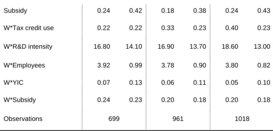
Subsidy 0.24 0.42 0.18 0.38 0.24 0.43

W*Tax credit use 0.22 0.22 0.33 0.23 0.40 0.23

W*R&D intensity 16.80 14.10 16.90 13.70 18.60 13.00

W*Employees 3.92 0.99 3.78 0.90 3.80 0.82

W*YIC 0.07 0.13 0.06 0.11 0.05 0.10

W*Subsidy 0.24 0.23 0.20 0.18 0.20 0.18

Observations 699 961 1018

Notes: * The percentage of first-time users is relative to the number of R&D active firms in the sample. In order to obtain the values from Table 2, row one needs to be divided by row two (slight differences will occur due to trimming decimals).

4.5.

Results

Table 4 illustrates the estimation results of equation (1) by the GS2SLS procedure26 with (columns 1c, 2c, 3c) and without (columns 1b, 2b, 3b) contextual effects. As a benchmark, we compare the latter results with the ones of a ‘naïve’ OLS model (models 1a, 2a, 3a), in which we do not instrument the endogenous peer effect27. We perform a yearly cross-sectional analysis due to the fact that we expect peer effects to behave differently in the first period after the introduction of the tax credit, when fewer companies knew of its existence, suggesting a greater potential for peer effects. We also assume that this different behaviour cannot be captured solely by year indicators.28 The first row shows the coefficient of the endogenous peer effect  from equation (1), while the subsequent rows show, respectively, the coefficients of the focal firm characteristics δ, and the parameter θ capturing the spatial correlation between the error terms from equation (3). Since the primary purpose of the contextual peer effects is to distinguish this influence from the endogenous peer effects, which capture the influence emanating from peers’ decisions and where our main interest lies, we omit them from the results presented here, but they are reported in Appendix in Table 8.

26 _{For the estimation of our model through GS2SLS, we use the R package sphet (Piras, 2010) and define}

endogenous peer effects as the (lagged) general use of tax credits by a firms’ peers, and also include lagged contextual effects.

27 _{We estimate an OLS model for comparability with our main GS2SLS specification, in line with our linear}

probability model. Alternatively, we have estimated the benchmark through a probit model, the results being higlhly similar in terms of significance and magnitude with the basic OLS estimation.

28 _{We have also estimated the model on the pooled cross-section, but failed to find significant endogenous peer}

19

Table 4 GS2SLS estimation of endogenous peer effects from the closest ten peers

2007 2009 2011

OLS GS2SLS OLS GS2SLS OLS GS2SLS

1a 1b 1c 2a 2b 2c 3a 3b 3c

Endogenous peer effect 0.106** 0.282*** 0.586** -0.006 -0.043 1.122** -0.018 0.016 0.103 (0.046) (0.106) (0.259) (0.045) (0.072) (0.562) (0.023) (0.046) (0.136) Log(Employees) 0.015** 0.012** 0.012** 0.019*** 0.019*** 0.020*** -0.001 -0.001 0.0003 (0.006) (0.006) (0.006) (0.007) (0.007) (0.007) (0.004) (0.003) (0.003) YIC 0.059 0.05 0.043 0.013 0.012 0.026 -0.027 -0.029*** -0.029*** (0.038) (0.040) (0.039) (0.044) (0.050) (0.055) (0.025) (0.009) (0.010) Subsidies 0.012 0.006 0.005 -0.039 -0.038 -0.060** -0.019 -0.021* -0.027*** (0.022) (0.023) (0.023) (0.024) (0.024) (0.028) (0.014) (0.012) (0.015) R&D Intensity -0.0005 -0.001** -0.001** 0.001** 0.001** 0.001 -0.0002 0.000 -0.0002 (0.0005) (0.000) (0.001) (0.001) (0.001) (0.001) (0.0003) (0.000) (0.0002) Spatial error θ 0.058 0.233*** 0.015 0.298** -0.025 0.020 (0.080) (0.091) (0.054) (0.120) (0.024) (0.048)

Notes: a) ***, **, and * indicate significance levels of 1%, 5% and 10%, respectively. b) Intercept estimated but not shown in table.

c) Standard errors in parentheses.

20

The GS2SLS estimates that include contextual and correlated effects (columns 1c, 2c, 3c) show positive and significant endogenous peer effects in 2007 and 2009, although we cannot reject the null hypothesis of no effects in 2011. The results indicate that a firm’s decision to start using R&D tax credits is positively influenced by the (lagged) average use of tax credits of up to ten of its closest peers within the same 3-digit NACE industry code, but primarily so in the first few years following the introduction of the measure.

With respect to firm characteristics explaining adoption of the R&D tax credit, we find that, on average, larger firms have a higher probability of being first-time users, while young innovative companies are less likely to adopt the tax credit in the latter period, as are subsidy users in 2009 and 2011. As argued in section 4.4, the result for YICs is consistent with the expectation that YICs are at the forefront to adopt new R&D support measures. Our data seems to capture periods when YICs are mostly general users of tax credits rather than adopters. Out of 43 YICs present in the data set in 2007, 15 were using the tax credit in general and only 3 were using it for the first time. Similarly, we observe 24 and 31 users and only 4 and 1 new adopters in 2009 and 2011 respectively29. This numbers suggest that we might fail to capture YIC adoption behaviour in years not covered by our data30. The same observation is true for subsidy users. In 2011, only 2 firms that had received subsidies one year before become adopters of tax credits, whereas there were 12 and 14 in 2007 and 2009 respectively31.

Somewhat contrary to expectations, more R&D intensive firms are also less likely to be adopters in the immediate period after introduction of the measure, although the coefficient’s magnitude is rather small. Moreover, since we are analysing a sample of R&D active firms that are – in principle – all eligible for the R&D tax credit, this variable acts a control rather than a fundamental driver of tax credit adoption32_.

29 _{The numbers are similar in terms of lagged YIC status, as the variable is used in our estimations. Moreover,}

of the adopters in 2011, none were YICs a year before.

30 _{Our data is based on the biannual Belgian OECD business R&D survey. Due to the low sample overlap}

between two consecutive surveys and the fact that we lag our explanatory variables, we decided to estimate cross sectional models on the periods with most coverage – 2007, 2009 and 2011.

31 _{The difference between adoption and general usage behaviour can also be seen in a pooled OLS estimation}

presented in Appendix in Table 9. The first column shows that (lagged) YIC status and subsidy use do not explain adoption behaviour (without accounting for peer effects), but they do significantly and positvely influence overall use of tax credits (column two).

32 _{We also observe in Table 9 in Appendix that the R&D intensity coefficient is significant at 1% in a simple}

OLS (excluding any peer effects) of general use of tax credits (column 2). Similarly, it positively affects adoption in 2009 (again, withoug considering peer effects), while in the other two periods – as well as in the pooled cross sections – it has very limited impact and no statistical significance at 10%.

21

In most studies implementing spatial estimators, interpreting the magnitude of the endogenous effect – or spatial lag – is cumbersome due to feedback loops – i.e. peers’ decisions affect the focal firm’s decision, which in turn affects its peers and so on. However, because our endogenous effect variable – average peer tax credit use – is measured prior to the dependent – first-time tax credit use – we avoid this issue of circularity. This facilitates the interpretation of the magnitude of the coefficients. In 2007, a 10% increase in the number of peers having used tax credits the year before increases the probability that the focal firm becomes a user by 5.86 percentage points (model 1c). Similarly, the effect amounts to 11.22 percentage points in 2009 (model 2c) and 1.03 percentage points in 2011 (model 3c), although the latter is not significantly different from zero. The magnitude of peer effects is quite large given that less than 10% of the sample firms in any given year adopt the tax credit. From a policy perspective, these effects indicate the presence of an important multiplier effect. More practically, it suggests that geographically targeted information campaigns can be very effective at increasing the take-up of tax credits. For example, ensuring that one in every ten firms knows about – and uses – the fiscal measure can increase adoption by as much as 11 percentage points, converting two out of ten firms doubles the take-up, and so forth.

4.6. Robustness checks

As mentioned in section 2, the definition of interactions between firms is based on their industry membership and geographical proximity. Notwithstanding that the definition is informed by theory, it is an assumption that we need to make in the absence of interaction patterns between firms.33 Thus, the network structure used for the analysis might only partially capture the true peer network. The spatial econometrics literature provides little guidance on the potential bias due to a misspecified spatial weights matrix 𝑊 and the resulting measurement error in the instruments. For the related SAR model without spatially correlated errors, Lee (2009) found bias from over-specification of the spatial weights matrix to be lower than bias from under-specification in both maximum likelihood and 2SLS estimation. To investigate potential implications of a misspecified peer network for our results, we perform the following robustness tests. First and foremost, following Helmers & Patnam (2014), we randomize peer groups by performing a permutation of firms over the two peer group dimensions, i.e. locations and industries, and then re-estimate the model. This falsification test

33 _{Note that the network structure might still be misspecified even if self-reported firm data were available, due to}

perception bias and other (un)intentional misreporting by firms on whether they were affected by other firms in their decisions to start using the R&D tax credit.

22

serves to verify that our result on peer effects is not obtained when considering any random peer group network. Second, we re-run the analysis for different peer group sizes to verify whether the results are not driven solely by the choice of a ten nearest neighbour network. Finally, we introduce additional controls in the model to check for industry-wide and regional effects on adoption behaviour that are not accounted for by the industry and location dimension of the peer group definitions.

4.6.1. Random peer assignment

To test the assumption of our industry- and location-based peer groups, we randomly assign ten peers to each firm in the sample by shuffling the locations and 3-digit NACE industry codes across firms. Although this method ensures that peers are random, it also maintains the basic structure of the sample – that is, each industry and municipality will keep the true number of firms, but firms are randomly along these dimensions.

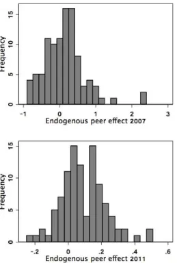
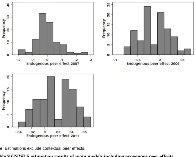
As for the main results, we estimate equation (1) using the GS2SLS method and we repeat the procedure 100 times, each repetition generating a new random network structure. The histograms in Figure 2 show the distribution of point estimates of the endogenous peer effects obtained in the 100 replications for each time period.34

34 _{We performed the same procedure for the model without the contextual effects} _{. The results are consistent with}

23

Figure 2 Histograms of point estimates of endogenous effects for 10 random peers

Note: Estimations include contextual peer effects.

The mean estimate of the endogenous peer effect is 0.139 (with a standard deviation of 0.560) for 2007, a mean of 0.105 (s.d. 0.590) for 2009, and a mean of 0.091 (s.d. 0.130) in 2011. These results imply that we cannot reject the null of zero endogenous peer effects in the randomised networks. Furthermore, 99% of point estimates are statistically insignificant at 10% level. We interpret this as reassuring evidence that our main model captures the underlying network structure of peer groups rather than some empirical artefact arising from a misspecified network.

4.6.2. Misspecification of peer group size

As explained in section 2, the empirical upper bound on the peer group size implied by our data is about ten peers, as this allows the identification of social effects by intransitivity for the majority of firms in the sample, while for a minority of firms identification is based on variation in the peer group size.35

24

We now restrict the maximum group size to five and seven firms and present the GS2SLS estimation results of endogenous peer effects in Table 11. The complete results – including exogenous effects and individual characteristics are included in Appendix in Table 11.

Table 5: Endogenous peer effect for different peer group sizes (K)

2007 2009 2011 K=10 0.586** 1.122** 0.103 (0.259) (0.562) (0.136) K=7 0.536* 2.325* 0.235 (0.309) (1.245) (0.227) K=5 0.453 -1.234 -0.152 (0.364) (1.867) (0.183)

Notes: a) ***, **, and * indicate significance levels of 1%, 5% and 10%, respectively. b) Standard errors in parentheses.

We observe that the endogenous effect for groups of seven peers follows our main results by having a positive and significant coefficient in the first two periods, followed by a non-significant and smaller effect in 2011. The same patterns arise in the case of contextual and correlated effects. However, when defining peer groups of five firms, we are unable to robustly identify the endogenous or exogenous effects.

These results indicate that groups of 10 peers are sufficiently broad containers of firm interaction while progressively smaller peer groups fail to capture peer effects.36 _{. Combined}

with the network scramble test, we are confident that the used peer groups capture the real network structure of firms sufficiently accurately. Similar patterns arising from under- and over-specification are noted by Lee (2009) and Helmers and Patnam (2014).

Furthermore, we have defined peer groups within 3-digit NACE code industries. Although we have based our choice on previous empirical evidence (e.g. Leary & Roberts, 2014), we now test whether choosing different definitions of industry boundaries also allow identify peer effects. Table 6 shows the results of GS2SLS estimations for K=10 and peers defined in the same 2 and 4-digit NACE sectors respectively. We observe that none of the endogenous peer effect coefficients are significant at 10% level, although they are similar in magnitude and yearly variation to our main results. These results build confidence in the fact that peer effects operate at 3-digit NACE sector level, as lower or higher granularity does not seem to capture any interaction between firms. Indeed, 2-digit NACE sectors may be too wide a definition,

36 _{Similar patterns arising from under- and over-specification of peer groups are reported by Lee (2009) and}

25

coupling together firms that in practice do not have any links, whereas 4-digit sectors are too narrow, which implies that there are missing links in networks defined at this level.

Table 6 GS2SLS estimations of peer effects with groups defined at 2 and 4-digit NACE sectors

2007 2009 2011 2-digit NACE 4-digit NACE 2-digit NACE 4-digit NACE 2-digit NACE 4-digit NACE (1) (2) (3) (4) (5) (6) Endogenous effect 0.371 0.405 1.781 0.271 0.261 -0.090 (0.467) (0.316) (1.682) (0.499) (0.191) (0.142) ln(employees) 0.012** 0.012* 0.022*** 0.016*** 0.000 -0.002 (0.006) (0.006) (0.008) (0.006) (0.003) (0.004) YIC 0.049 0.031 0.019 -0.010 -0.027*** -0.023** (0.041) (0.037) (0.060) (0.051) (0.010) (0.010) Subsidy 0.014 0.005 -0.071** -0.051* -0.026** -0.016 (0.022) (0.025) (0.030) (0.027) (0.012) (0.012) R&D intensity -0.001 -0.0008* 0.001* 0.001 0.000 0.000 (0.000) (0.000) (0.000) (0.000) (0.000) (0.000)

Notes: a) ***, **, and * indicate significance levels of 1%, 5% and 10%, respectively. b) Standard errors in parentheses.

c) Contextual effects, spatial errors and intercept estimated but not shown - see Table 12 in Appendix.

4.6.3. Omitted control variables

Finally, we test how robust our results are to omitted variable bias. We have mentioned in the Data section that we do not specifically control for industry and geographical region because these two dimensions are part of the definition of peer groups. Since there may exist region- and industry-wide influences that extend beyond the reach of the peer group and that may lead firms to adopt the tax credit, we now re-estimate the spatial model by including binary indicators for the three geographical-administrative regions – Brussels (baseline), Wallonia and Flanders – as well as for industries aggregated into four groups – high- and low-tech manufacturing and services. Although including these covariates reduces the identifying variation of the endogenous and exogenous effects, the coefficients remain robust and show similar values and significance to the main specification, as can be seen in Table 7. Moreover, the included region indicators are not significant, with one exception, strengthening our trust in our main specification. Similarly, industry affiliation seems to matter little in firms’ use of tax credits, as we only find some evidence in 2009 of firms in high-tech services and low-tech manufacturing sectors having higher probability of adopting R&D tax credits.

26

Table 7 Estimation of endogenous and exogenous peer effects from the closest ten peers including industry and region indicators

2007 2009 2011 Endogenous effect 0.672** 1.350* 0.177 (0.313) (0.798) (0.156) R&D intensity -0.001* 0.001 0.000 (0.000) (0.001) (0.000) Log(Employees) 0.010 0.022*** -0.001 (0.007) (0.008) (0.004) YIC 0.035 -0.026 -0.026** (0.039) (0.060) (0.013) Subsidies 0.004 -0.044 -0.036** (0.024) (0.028) (0.016) Flanders Region -0.008 0.000 -0.008 (0.030) (0.040) (0.025) Wallonia Region -0.059 -0.031 -0.043* (0.041) (0.066) (0.026) High-tech services 0.029 0.287* 0.004 (0.050) (0.152) (0.021) Low-tech manufact. 0.082 0.241** 0.004 (0.056) (0.116) (0.017) Low-tech services 0.006 0.149 0.025 (0.045) (0.093) (0.022)

Notes: a) ***, **, and * indicate significance levels of 1%, 5% and 10%, respectively.

b) Intercept, contextual effects and spatially-lagged errors  estimated but not shown in table – see Table 13 in Appendix for full results.

c) Standard errors in parentheses.

5. Conclusions

While our analysis does not directly answer the puzzling question why firms seem reluctant to make use of a public support measure that clearly benefits them, it shows how peer influence among firms fosters the adoption of R&D tax credits. Our empirical application uses a methodologically innovative approach to identify these peer effects: by making the plausible assumption of not fully overlapping peer groups based on distance and industry, this paper is the first to show how peer effects play a role in firms’ response to R&D public support schemes

27

in the absence of clear peer group information. In particular, we show that firms optimize their R&D costs through public support as information from their peers reaches them. Consistent with a bounded rationality perspective, we interpret this as a way for firms to cope with the multitude of public support measures they face, and which are not always efficiently ‘marketed’ by public authorities. We have also shown that a critical mass of peers is required to find such effects. Using intransitivity in the network structure to separate endogenous peer effects (peers’ decisions) from exogenous peer effects (peers’ characteristics), the results show that these are two separate channels through which peers influence peers influence firms’ decision making.

Second, positive peer effects in firms’ decisions to adopt public support for R&D are important given the tenacious proliferation and fragmentation of public support schemes, which is believed to create a situation that bewilders some firms. In particular, while our findings do not imply policy interventions with respect to R&D support schemes as such, they are suggestive of opportunities to foster adoption of public support for R&D. For example, these insights can be used to set up more effective government communication initiatives, such that early adopters in different industries are involved in promoting the measures to their respective peers. More specifically, adoption by eligible firms could be expedited by communicating the measure to sufficiently fine-grained sectors and in a geographical distributed way. As opposed to broad policy communications, ‘narrowcasting’ would help to reach many localized firm clusters, or peer groups, allowing for rapid peer-to-peer influence, once initial adoption has taken place. Third, the establishment of peer effects as a significant factor driving firms’ selection into support schemes informs the methodological literature on selection bias in program evaluation (Imbens & Wooldridge, 2009). Namely, the existence of peer effects calls for looking beyond the individual firm to explain selection into support programs. More specifically, peer effects could be accounted for in the selection equation when estimating the effects of policy interventions in R&D, especially in contexts where there is reason to believe information about support measures has not reached all potential users. Including peer effects as an explanatory factor for firm participation in a programme will then help to satisfy the conditional independence assumption underlying matching estimators, or to identify the parameters of the selection equation in two-step estimations.

Finally, this paper contributes to the broader literature on peer effects between firms. Given the high degree of clustering in many ‘small world’ firm networks (Fleming & Marx, 2006), our approach of exploiting intransitivity in firms’ networks is more generally applicable to identify