Modelling of geotechnical problems using soft computing

Modelling of Geotechnical Problems

using Soft Computing

A Thesis Submitted in Partial Fulfillment of the Requirements for the

Degree of

Master of Technology

in

Civil Engineering

SUNIL KHUNTIA

DEPARTMENT OF CIVIL ENGINEERING

NATIONAL INSTITUTE OF TECHNOLOGY, ROURKELA

2014

Modelling of Geotechnical Problems using

Soft Computing

A Thesis Submitted in Partial Fulfillment of the Requirements for the

Degree of

Master of Technology

in

Civil Engineering

Under the guidance and supervision of

Prof. Chittaranjan Patra

Submitted By

Sunil Khuntia

DEPARTMENT OF CIVIL ENGINEERING

NATIONAL INSTITUTE OF TECHNOLOGY, ROURKELA

2014

CERTIFICATE

This is to certify that the thesis entitled “Modelling of Geotechnical Problems using Soft Computing” being submitted by Sunil Khuntia in partial fulfillment of the requirements for the honor of Master of Technology Degree in

Civil Engineering with specialization in Geotechnical Engineering at National

Institute of Technology, Rourkela, is an authentic work completed by him under my

guidance and supervision.

To the best of my knowledge, the matter exemplified in this report has not been

submitted to any other university/institute for the award of any degree or diploma.

Place: Rourkela Date:

Prof. Chittaranjan Patra Department of Civil Engineering

ACKNOWLEDGEMENT

I earnestly express my profound feeling of appreciation to my thesis supervisor,

Prof. Chittaranjan Patra for his master direction, constant support and spark all around

the course of postulation work. I am genuinely grateful for his educated backing and

imaginative feedback, which headed me to create my thoughts and made my work

fascinating and agreeable.

I might additionally want to express my profound thankfulness and earnest

because of Prof. N. Roy, Head, Civil Engineering Department, Prof. S.P. Singh, Prof. S.

K. Das and Prof. R. N. Behera of Civil Engineering for giving different varieties of

conceivable help and consolation. I am obliged to every one of them and NIT Rourkela

for providing for me the essentials and opportunity to execute them.

I want to take this probability to thank my parents and my sister for their

unconditional love, moral support and encouragement for the completion of this specific

project.

I ought to express my genuine because of all my nearby companions and seniors

in light of their ethical backing and advices throughout my M-Tech project.

Table of Contents

Abstract... i

List of Figures... iii

List of Tables ... v CHAPTER 1 ... 1 INTRODUCTION ... 1 1.1 Introduction ... 1 1.2 Origin of Project ... 2 1.3 Objective ... 2

1.4 Applications in Geotechnical Engineering... 3

1.5 Methodology for Soft-Computing... 3

1.6 Software used ... 3

CHAPTER 2 ... 4

METHODOLOGY ... 4

2.1 Artificial Neural Network (ANNs) ... 4

2.1.1 An overview of ANNs ... 4

2.1.2 Basic Concepts of ANNs ... 5

2.1.3 ANN Model Equation... 7

2.1.4 Methodology of ANN ... 8

2.2 Details of Support Vector Machine (SVM) ... 10

2.2.1 Support Vector Machine (SVM) ... 10

2.2.2 Least Square Support Vector Machine (LS SVM) ... 14

2.3 Multivariate Adaptive Regression Splines (MARS) ... 15

2.4 Performance criteria ... 17

2.5 Sensitivity analysis ... 18

2.5.1 Variance based sensitivity analysis ... 18

2.5.2 Rate of change of input... 19

2.5.3 Connection weight approach ... 19

2.5.4 Garson‟s algorithm ... 19

CHAPTER 3 ... 22

PREDICTION OF COMPACTION PARAMETERS OF SANDY SOIL ... 22

3.1 Introduction ... 22

3.2 Database preprocessing ... 26

3.3.1 ANN model equation ... 26

3.3.2 LS-SVM model equation ... 27

3.3.3 MARS model equation ... 28

3.4 Performance comparison among all the models ... 29

3.5 Sensitivity Analysis ... 34

3.6 Discussion ... 35

CHAPTER 4 ... 36

PREDICTION OF RELATIVE DENSITY OF CLEAN SAND ... 36

4.1 Introduction ... 36

4.2 Selection of the input parameters ... 36

4.3 Database preprocessing ... 37

4.4 Different developed model equations ... 42

4.4.1 ANN Model equation ... 42

4.4.2 LS-SVM Model equation ... 42

4.4.3 MARS model equation ... 43

4.5 Result comparison and discussion ... 44

4.6 Sensitivity Analysis ... 47

4.7 Discussion ... 48

CHAPTER 5 ... 49

PREDICTION OF COMPRESSION INDEX OF CLAY ... 49

5.1 Introduction ... 49

5.2 Data base selection ... 50

5.3 Database preprocessing ... 51

5.4 Different developed model equations ... 54

5.4.1 ANN Model equation ... 55

5.4.2 LS-SVM Model equation ... 55

5.4.3 MARS model equation ... 56

5.5 Results and discussion ... 57

5.6 Sensitivity Analysis ... 60

5.7 Discussions ... 61

CHAPTER 6 ... 62

PREDICTION OF SIDE RESISTANCE OF DRILLED SHAFT ... 62

6.2 Database used in present study ... 63

6.3 Database preprocessing ... 63

6.4 Different developed model equations ... 65

6.4.1 LS-SVM Model equation ... 65

6.4.2 MARS model equation ... 66

6.5 Result comparison ... 66

6.6 Sensitivity of the parameters ... 68

6.7 Discussion ... 69

CHAPTER 7 ... 70

CONCLUSION AND FUTURE SCOPE ... 70

7.1 Conclusion ... 70

7.2 Future scope for research ... 70

i

Abstract

Correlations are very significant from the earliest days; in some cases, it is

essential as it is difficult to measure the amount directly, and in other cases it is

desirable to ascertain the results with other tests through correlations. Soft computing

techniques are now being used as alternate statistical tool, and new techniques such as

artificial neural networks (ANN), support vector machine (SVM), multivariate adaptive

regression splines (MARS) has been employed for developing the predictive models to

estimate the needed parameters. In this report, four geotechnical problems like

compaction parameters of sandy soil, compression index of clay, relative density of

clean sand and side resistance of drilled shaft have been modeled. In the first problem,

compaction parameters (i.e. MDD and OMC) of sandy soil have been predicted from its

index properties such as coefficient of uniformity, percentage of sand and fines content

with reference to compactive effort and MARS shows better predictability. In the

second problem, the relative density (Dr) of clean sand has been predicted from

coefficient of uniformity, mean diameter of grain size with reference to four levels of

compactive effort and predictability of LS-SVM is found to be very accurate. In third

problem, compression index of clay has been predicted from consistency limits, natural

moisture content and initial void ratio and the developed ANN shows better prediction.

In the fourth problem, side resistance of drilled shaft has been predicted from effective

stress and undrained shear strength and the MARS model performs better than the other

models. Various error criteria such as mean absolute error (MAE), root mean square

error (RMSE), mean absolute percentage error (MAPE) and correlation coefficient (R)

have been considered for the comparison of different models. Finally different

sensitivity analysis has been shown to identify the significance of different input

ii

the soft computing system is a good tool for minimizing the uncertainties in the soil

engineering projects. The use of soft computing may provide new approaches and

iii

List of Figures

Figure 2.1 Generic processing element of neural network Figure 2.2 Flow chart of neural network modelling Figure 2.3 Soft margin loss setting for a linear SVM

Figure 2.4 Steps for connection weight approach and Garson‟s algorithm (Olden, Joy and Death, 2004)

Figure 3.1 Corresponding α-values in the prediction of MDD

Figure 3.2 Corresponding α-values in the prediction of OMC

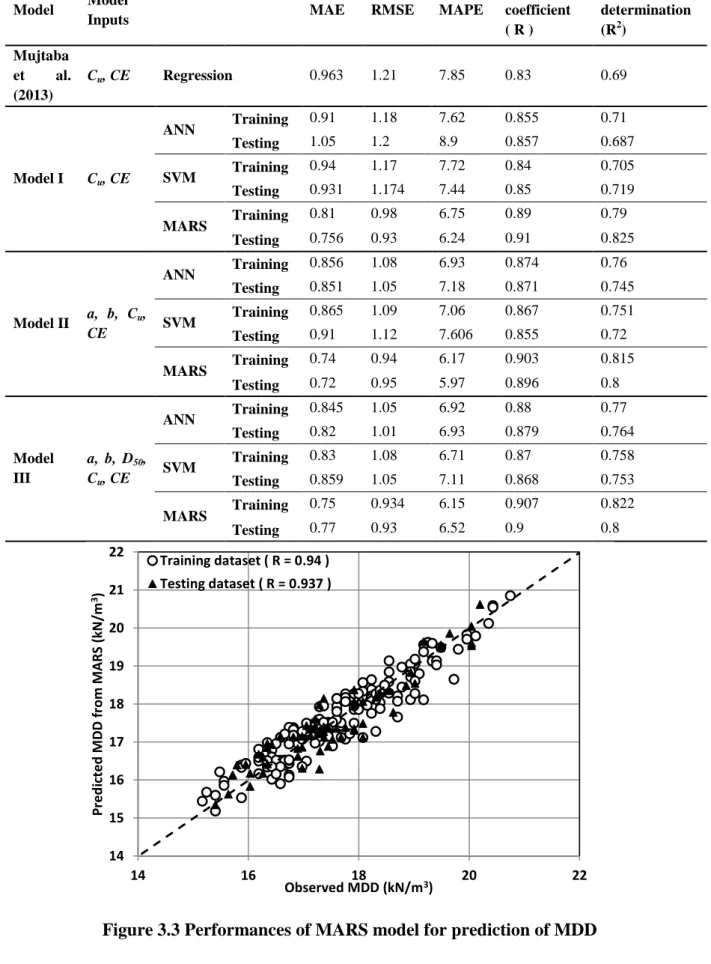
Figure 3.3 Performances of MARS model for prediction of MDD Figure 3.4 Performances of MARS model for prediction of OMC

Figure 3.5 Comparison between actual and predicted value of MDD using MARS Figure 3.6 Comparison between actual and predicted value of OMC using MARS Figure 3.7 Comparison between different models in terms of (a) MAPE and (b) RMSE

for the prediction of MDD.

Figure 3.8 Comparison of different models in terms of (a) MAPE and (b) RMSE for the prediction of OMC

Figure 3.9 Sensitivity of the parameters in prediction of MDD and OMC Figure 4.1 Corresponding α-value for the LS-SVM model for prediction of Dr

Figure 4.2 Comparison of MAPE of different models in the prediction of Dr

Figure 4.3 Comparison of RMSE of different models in the prediction of Dr

Figure 4.4 Comparison between experimental and predicted value of Dr (Patra et al., 2010).

Figure 4.5 Performance of the LS-SVM model in training and testing (Present study). Figure 4.6 Variation of the values predicted by LS-SVM model and observed values.

Figure 4.7 Sensitivity of the parameters

Figure 5.1 Corresponding α-values in the LS-SVM model

Figure 5.2 Performance evaluations of different models in terms of (a) MAPE and (b) RMSE

Figure 5.3 Performance of model 3 using ANN in training and testing.

Figure 5.4 Variation of actual and predicted value from ANN of compression index Figure 5.5 Sensitivity of different parameters

iv

Figure 6.2 Comparison between models in terms of MAPE

Figure 6.3 Comparison between models in terms of RMSE

Figure 6.4 Performance of MARS model in the prediction

Figure 6.5 Comparison between observed and predicted values

v

List of Tables

Table 3.1 Some of the compaction of test data and index properties of soil

Table 3.2 Summary of Statistical values of input and output parameters

Table 3.3 Cross correlation between the inputs and output

Table 3.4 Basis functions of MARS model

Table 3.5 Results of Different Models for Prediction of MDD of sandy soil

Table 3.6 Results of Different Models for Prediction of OMC of sandy soil Table 4.1 Statistical values of parameters

Table 4.2 Cross-correlation between different parameters

Table 4.3 Training database considered for the model development

Table 4.4 Results of Different Models for Prediction of Relative density of clean sand

Table 5.1 Cross-correlation matrix for all data Table 5.2 Statistical value of the parameters

Table 5.3 Database considered for modeling for training

Table 5.4 Results of Different Models for Prediction of compression index of clay

Table 5.5 Some widely used empirical correlations

Table 5.6 Results of different models for prediction of compression index of clay Table 5.7 Relative importance of different inputs as per Garson's algorithm and

connection weight approach

Table 6.1 Training dataset used in the modelling Table 6.2 Performances of different models

1

CHAPTER 1

INTRODUCTION

1.1 Introduction

In geotechnical engineering, empirical connections are frequently used to evaluate

certain engineering properties of soils. By means of data from extensive laboratory or field

testing, these correlations are generally derived with the help of statistical methods. Artificial

neural networks (ANNs), support vector machine (SVM) and multivariate adaptive

regression splines (MARS) are the forms of artificial intelligence. These techniques learn

from data cases presented to them in order to capture the functional interactions among the

data even if the fundamental relationships are unknown or the physical meaning is tough to

explain. This is in contrast to most traditional empirical and statistical methods, which need

prior information about the nature of the relationships among the data. AI i s thus well

suited to model the complex performance of most geotechnical engineering materials which,

by their very nature, exhibit extreme erraticism. This modeling capability, as well as the

ability to learn from experience, have given AI superiority over most traditional modeling

approaches since there is no need for making assumptions about what the primary rules

that govern the problem in hand could be.

ANN is still considered as „black box‟ system with poor simplification, though various

efforts made for modification and explanations. Recently support vector machine (SVM),

based on statistical learning theory and structural risk minimization is being used as an

alternate prediction model. The SVM uses constrained minimization, penalizing the error

margin during training. The error function being a convex function better generalization

used to observe in SVM compared to ANN.

Though AI techniques has proved to have the superior predictive capability than

2

materials, still it is facing some criticism due to the lack of transparency, knowledge

extraction and model uncertainty. To overcome this there is a development of improvised AI

techniques.

1.2 Origin of Project

• Empirical relationships are frequently used to estimate certain engineering properties of soils in geotechnical engineering.

• Computational techniques learn from data samples presented to them in order to capture the functional relationships among the data even if the fundamental relationships are

unknown or the physical sense is difficult to clarify.

• Most traditional empirical and statistical methods need prior knowledge about the nature of the interactions among the data.

• Soft-computing techniques are suitable to model the complex behavior of most geotechnical engineering materials which exhibit extreme inconsistency.

1.3 Objective

 To apply various soft-computing techniques like ANN, MARS and SVM in parametric estimation of Geotechnical problems.

 To model for relative density of granular soil from grain size distribution and compaction energy.

 To model for compaction parameters (Maximum Dry Density and Optimum Moisture Content) of granular and c-ϕ soils from index properties and compaction energy.

 To model for compression Index from various physical properties of clayey soil.

 To model the side resistance of drilled shaft from effective stress and undrained shear strength.

3

1.4 Applications in Geotechnical Engineering

Various geotechnical problems where soft computing has been applied are:

 For forecasting the axial and lateral load capacities in compression and uplift of pile foundations.

 Conventional constitutive modeling based on the elasticity and plasticity theories to properly simulate the performance of geomaterials.

 For estimating several soil properties including the shear strength, stress history, pre-consolidation pressure, swell pressure, compaction and permeability, soil

classification and soil density.

 Predicting liquefaction potential.

 Bearing capacity and Settlement prediction of shallow foundations.

 Other applications of Artificial Intelligence in geotechnical engineering include retaining walls, dams, blasting, mining, geo-environmental engineering, rock

mechanics, site characterization, tunnels and underground openings and slope

stability.

1.5 Methodology for Soft-Computing

• Artificial Neural Network (ANN)

• A universal function approximator and fast to evaluate new examples.

• Multivariate Adaptive Regression Splines (MARS)

• Capacity to find complex data mapping and produce simple, easy-to-interpret models.

• Support Vector Machine

• The quality of generalization and ease of training of SVM is better.

1.6 Software used

4

CHAPTER 2

METHODOLOGY

2.1 Artificial Neural Network (ANNs)

2.1.1 An overview of ANNs

In the last decades, Artificial Intelligence (AI) techniques such as Artificial Neural

Networks (ANNs) have received a great deal of attention. In essence, ANN is an information

technology that mimics the human brain and nervous system in learning from experience and

generalizes from previous examples to generate new outputs by abstracting essential

characteristics from inputs in the pattern of variable interconnection weights among the

processing elements. ANNs are more powerful than traditional methods in the situations

when the problem requires qualitative or complex quantitative reasoning where the

conventional statistical and mathematical methods are inadequate or the parameters are

highly interdependent and data is intrinsically noisy, incomplete or error prone (Bailey and

Thompson, 1990).

ANNs have many advantages over traditional methods of modeling. Firstly, as

opposed to the traditional mathematical and statistical methods, ANNs are data-driven

self-adaptive methods, which can capture subtle functional relationships among the data even if

the underlying relationships are unknown or hard to describe. Secondly, ANNs are able to

capture complex nonlinear relationship with better accuracy (Rumelhart et al. 1994). Thirdly,

the most important advantage of ANNs over mathematical and statistical models is their

adaptability. ANN systems can automatically adjust their weights to optimize their behavior

(Boussabaine, 1996). Neural networks have been utilized for classification, clustering, vector

5

2.1.2 Basic Concepts of ANNs

An artificial neural network is a computational model defined by four parameters:

type of neurons, connection architecture, learning algorithm and recall algorithm (Mehrotra,

et al., 1997).

2.1.2.1 Artificial Neural Systems

ANNs is an information processing technology that simulates the human nervous

system. It is built on three basic components: processing elements (PE) which are an artificial model of human neuron, interconnections whose functions are similar to the axon and

synapses which are the junctions where an interconnection meets a PE. Each PE receives signals from other PEs that constitute an input pattern. This input pattern stimulates the PE to

reach some level of activity. If the activity is strong enough, the PE generates a single output

signal that is transmitted to other PEs through an interconnection.

2.1.2.2 Processing Elements

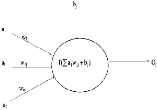
Figure 1 describes a typical artificial neuron. The input signals come from either the

environment or outputs of other PEs and form an input vector:

A





input connections: w₁,w₂,....,w_n. The neuron has a bias b. The sum of the weighted inputs and the bias form the net input signal, X:

b A W a w b X n i i ij j    



The input signal is then sent to a transfer function, which serves as a non-linear

threshold. The transfer function calculates output signal of the PE (j) as:

) (X f

6

Where Oj is the output signal from PE(j); f is a transfer function and X is the net input

signal to PE(j).

Figure 2.1 Generic processing element of neural network 2.1.2.3 Threshold functions

There are many threshold functions adopted in ANNs. The two most commonly used

transfer functions are linear and sigmoid.

 The linear threshold function: f(x) = x

 The sigmoid function: Log-sigmoid transfer function and Tan-Sigmoid transfer function is commonly used in backpropagation networks, partly because in backpropagation, it is important to be able to calculate the derivatives of any transfer function used (Demuth

and Beale, 2000). They can be expressed as the following equations:

Logistic function: _x e x f _   1 1 ) ( Hyperbolic tangent: _{x x} x x e e e e x f _     ) ( 2.1.2.4 Architecture of ANNs

The architecture of an ANN is the organization that assembles PEs into layers and

links them with weighted interconnections. The architecture determines how computations

proceed. A common ANN architecture is determined by three distinguishing characteristics:

7

The most commonly used ANN paradigm is multilayer perceptions (MLPs). A MLP

consists of an input layer, at least one hidden layer and one output layer. The neurons in each

layer are usually fully connected to the neurons in another layer. Among them, three-layer

feed forward network is the most popular. Feed forward network is a type of network in

which connection is allowed from a node in layer i only to nodes in layer i+1. The three

layers are input layer, hidden layer and output layer. Input layer is the layer that receives

input signals from the environment. Output layer is the layer that emits signals to the

environment. Hidden layers are layers between the input and output layers.

2.1.2.5 Learning Rules

Learning makes possible modification of behavior in response to the environment. A

learning rule is a procedure for modifying the weights of connections between the nodes and

biases of a network. These are three broad learning categories: supervised learning,

unsupervised learning and reinforcement learning.

2.1.3 ANN Model Equation

A model equation is developed using the weights from trained neural network model

(Goh et al. 2005). The mathematical equation relating input parameters to output parameter

can be written as                       





where y = predicted value of output, fn = transfer function, h = no. of neurons in the

hidden layer, Xi = value of Inputs, m= no of input variables, wik = connection weight between

ith layer of input and kth neuron of hidden layer, wk = connection weight between kth neuron of

hidden layer and single output neuron, bhk = bias at the kth neuron of hidden layer and b0 =

8

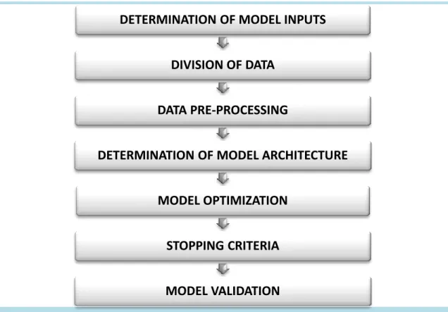
2.1.4 Methodology of ANN

The sequences of modeling by ANN are given in the flow chart below.

Figure 2.2 Flow chart of neural network modelling 2.1.4.1 Determination of Model Inputs

A subset of input variables can significantly improve model performance. A large

number of input variables usually increase the network size, resulting in a decrease in

processing speed and a reduction in the efficiency of the network. Another approach is to

train with different combinations of input variables and to select the network that has the best

performance. The network that performs the best is then retained. This process is repeated

for an increasing number of input variables, until the addition of other variables results in no

improvement in model performance.

2.1.4.2 Division of Data

ANNs accomplish best when they do not generalize beyond the range of the data used

for standardization. Therefore, the purpose of ANNs is to non-linearly introduce (generalize) DETERMINATION OF MODEL INPUTS

DIVISION OF DATA

DATA PRE-PROCESSING

DETERMINATION OF MODEL ARCHITECTURE

MODEL OPTIMIZATION

STOPPING CRITERIA

9

in high-dimensional space between the data used for calibration. A discrete validation set is

needed to ensure that the model can generalize within the range of the data used for

calibration. It is common practice to split the existing data into two subsets; a training set, to

construct the neural network model, and an independent validation set to evaluate the model

performance. Usually, two-thirds of the data are suggested for model training and one-third

for validation.

2.1.4.3 Data Pre-processing

Once the presented data have been divided into their subsets (i.e. training, testing

and validation), it is significant to process the data in a appropriate form. Data

pre-processing is necessary to ensure all variables obtain equal attention during the training

process and it usually speeds up the learning process. Pre-processing can be in the form of

data scaling, normalization and transformation. Scaling the output data is essential, as they

have to be equal with the limits of the transfer functions used in the output layer (e.g.

between –1.0 to 1.0 for the tanh transfer function and 0.0 to 1.0 for the sigmoid transfer

function). In some cases, the input data need to be normally distributed in order to obtain

optimal results. To improve the performance, transformation of the input data can be done to

some known forms (i.e. linear, log, exponential, etc.).

2.1.4.4 Determination of model architecture

Determining the network architecture is most essential and difficult job in ANN

model development. It needs selection of the ideal number of layers and the number of

nodes. It is usually achieved by fixing the number of layers and choosing the number of

nodes in each layer. For MLPs, there are always two layers signifying the input and output

variables in any neural network.

2.1.4.5 Model optimization

10

The aim is to find a global solution to what is usually a highly non-linear optimization

problem. The technique most commonly used for finding the optimum weight grouping of

feed-forward MLP neural networks is the back-propagation algorithm.

2.1.4.6 Stopping criteria

Stopping criteria are used to adopt when to break the training process. They

determine whether the model has been optimally or sub-optimally trained. Training can be

stopped: after the performance of a fixed number of training records; when the training error

reaches an effectively small value; or when no or minor changes in the training error

occur.

2.1.4.7 Model Validation

Once the training segment of the model has been effectively accomplished, the

performance of the trained model should be validated. The purpose of the model validation

phase is to confirm that the model has the ability to simplify within the limits set by the

training data. The error criteria such as coefficient of correlation (R), the root mean squared error (RMSE), and the mean absolute error (MAE) are often used to evaluate the

performance of models. The coefficient of correlation is a measure that is used to determine

the relative correlation and the goodness-of-fit between the expected and experimental

data.

2.2 Details of Support Vector Machine (SVM)

2.2.1 Support Vector Machine (SVM)

SVM has been utilized to solve a regression problem. Let us consider a training set

(x₁, y₁), (x₂, y₂)...(x_{N , yN}) from a vector, x_i ∈Rn with corresponding targets y_i, i = 1, 2, . . . , N . ε-SVR determines a linear function defined on x_i as,

f (x) = (w, x) + b (1.5) where w is a high-dimensional weight vector and b ∈ R as the bias such that there is

11

at most ε distance from the actual data and f (X ) should be flat. (.) denotes the dot product. No care is taken as long as errors are less than ε. But, any deviation more than ε is not

accepted. Flatness means the value of w should be as small as possible. This can be written as

convex optimization problem:

2 2 1 w Minimize Subjected to{ 〈 〉 〈 〉

In this case it is assumed that a function f exists which approximates the data set (_{xi, yi}) with ε precision. Introducing slack variables ξ_i, the problem can be stated as,

Minimize 



The parameter C controls the trade-off between the flatness of f and tolerance level of error ε. This deals with a ε-insensitive loss function expressed as,

| | {_{| |} | |

The graphical presentation of the ε-insensitive loss function is shown in the Figure 2.3. The opt i m i z at i o n probl em defined in (6) is easily solved in its dual formulation. The dual optimization problem can be written as ,

12

Figure 2.3 Soft margin loss setting for a linear SVM

Maximize {









 

where are Lagrange multipliers. In the above equations _xi and _xj are input vector spaces.

To address nonl inear regression problems, the linear SVR i s prolonged to

nonlinear SVR by mapping the input space into a high dimensional feature space through a

kernel function φ(x). In such case, (x, xt) is replaced by k(x, xt). Distinctive kernel functions used in the SVR are RBF, p o l yn o m i a l , linear and defined as,

Polynomial Kernel

In machine learning, the polynomial kernel is a kernel function commonly used with support vector machines (SVMs) and other kernelized models, that represents the

similarity of vectors (training samples) in a feature space over polynomials of the original

13

only at the given features of input samples to determine their similarity, but also

combinations of these.

For degree-d polynomials, the polynomial kernel is defined as

K(x,y)(xTyc)d _(1.8) where x and y are vectors in the input space, i.e. vectors of features computed from

training or test samples. c0is a constant trading off the influence of higher-order versus lower order terms in the polynomial. When c = 0, the kernel is called homogenous. (A further

generalized poly-kernel divides xTy by a user-specified scalar parameter a.)

As a kernel, K corresponds an inner product in a feature space based on some mapping φ:

K

 

The nature of φ can be glanced from an example. Let d = 2, so we get the special case of the quadratic kernel. Then





 



Radial Basis Function Kernel

In machine learning, the (Gaussian) radial basis function kernel, or RBF kernel, is a popular kernel function used in support vector machine classification.

The RBF kernel on two samples x and x', represented as feature vectors in some input space, is defined as _       _   ₂ 2 2 2 ' exp ) ' , (  x x x x K (1.10)

where xx' 2₂ may be recognized as the squared Euclidean distance between the two feature vectors. σ is a free parameter. The parameter σ in represents the spread of Gaussian kernel.

14

An equivalent, but simpler definition involves a parameter : 2 1 2   K(x,x')exp( xx'2₂) (1.11)

Since the value of the RBF kernel decreases with distance and ranges between zero

(in the limit) and one (when x = x'), it has a ready interpretation as a similarity measure. The feature space of the kernel has an infinite number of dimensions; for 1, its expansion is:



2.2.2 Least Square Support Vector Machine (LS SVM)

LSSVM models are an alternate formulation of SVM regression (Vapnik and Lerner,

1963) proposed by Suykens et al. (2002). Consider a given training set of N data points





x , _1with input data x_kRNand output y_krwhere RNthe N-dimensional vector space is and r is the one-dimensional vector space. For prediction of output using multiple parameters,





x _andy





In feature space LSSVM models take the form

b x w x

y( ) T( ) (1.13) Where the non-linear mapping (.) maps the input data into a higher dimensional feature space; wRn;br;w= an adjustable weight vector; b = the scalar threshold. In LSSVM for function estimation the following optimization problem is formulated:

Minimize:



15

for output prediction has been obtained by solving the above optimization problem (Scholkopf

and Smola, 2002; Vapnik, 1988).























_





σ

exp

,

x

x

x

x

K

σ is the width of radial basis function and αk is the Lagrange multiplier.

In LS-SVM regression algorithm, the regularization parameter γ and RBF kernel parameter σ2 have to be tuned in order to achieve an accurate solution. An integrated parameter optimization approach via simplex i.e. multidimensional unconstrained non-linear

optimization (Nelder and Mead 1965) and 10 fold cross-validation is used to minimize

generalization error. The optimum values of parameters [γ, σ2] and bias values have been used for the models developed herein.

2.3 Multivariate Adaptive Regression Splines (MARS)

MARS is a non-parametric regression technique introduced by Friedman (1991). It

essentially detects relation between a dependent variable and a set of predictors by fitting

piecewise linear regressions. In particular, MARS builds flexible models by dividing the

whole space of each covariate into various subsets and then defining a different regression

equation for each area. In this way, separate regression slopes in distinct intervals of the

predictors space are individuated (Hastie et al. 2009). A key concept is the notion of knots

that are the points that bound each interval of data in which a distinct regression equation is

calculated, i.e. where the behavior of the modelled function changes.

In this way, the space of predictors is split into several regions in which truncated

spline functions or basis functions (BFs) are fit. A truncated BF consists of a left-sided (1.17)

16

























where

b

(

x



t

)

b

(

x



t

)

degree of smoothness of the resultant regression models. The general MARS model equation

is given as

∑

where yp is the dependent variable predicted through the MARS model, M is the

number of BFs included into the model, α0 is the constant term, αm is the coefficient of the

mth truncated BF and Bm(x) is the mth truncated BF that may be a single spline function or a

product (interaction) of two or more spline functions.

The optimal MARS model is built by a two-stage process: a forward selection

procedure followed by a backward-pruning procedure. The forward procedure starts with just

the constant term in the model and then, by an iterative way, selects the best pairs of BFs that

improves the global model. This forward stepwise selection of BFs leads to a very complex

and over fitted model that has poor predictive abilities for new data. So, in the backward stage, the “lack of fit” criterion is used to evaluate the contribution of each BF to the descriptive abilities of the model and the BFs with the lowest contribution are removed one at

a time.

The “lack of fit” criterion used by MARS is the generalized cross-validation (GCV) criterion, i.e. the mean square error divided by a penalty dependent on the model complexity.

17

 





 



Where n is the number of observations in the data set, M is the number of

non-constant BFs, and C(M) is the cost-complexity measure of the model containing M BFs.

C(M) increases with the number of BFs and has the purpose to penalize model complexity in

order to avoid over-fitting. It is defined as:

C(M) = M +d x M (1.21)

Where d is a cost penalty factor for adding a BF. The higher value of d reduces the

number of BFs in the final model.

2.4 Performance criteria

The present study uses various statistical error measure criterions like R, MAPE and

RMSE to compare different developed models. A good model should have; R value

(expresses degree of similarity between predicted and actual values) close to 1 and low

MAPE and RMSE values (indicate high confidence in model-predicted values).

Root mean-squared error (RMSE) is used to compute the square error of the prediction compared to actual values as well as the square root of the summation value. Thus the RMSE

is expressed using the following equation:







Mean Absolute Percentage Error (MAPE) is a measure of closeness of predictions to actual values. The mean absolute error is given by





















y

y

y

n

MAPE

100

1

18

The Coefficient of correlation (R) value is a measure of linear relationship between the predictions and the actual values. The R value is calculated using the following formula:

] ) ( [ ] ) ( [ ) ( ) ( ) . ( 2 2 2 2











 

Mean of the observed data =



Total sum of squares =



Explained sum of squares =



Residual sum of squares =



where y and yp are the actual and the predicted values;

y

y

actual and the predicted values respectively; n is the sample size.

2.5 Sensitivity analysis

Different methods have been adopted for knowing the importance of the input

parameters for the developed models.

2.5.1 Variance based sensitivity analysis

Iman and Hora (1990) investigate the performance of a sensitivity measure based on

the percentage variance in f explained by any variable Xi. This technique is known as measure of importance, and its use is associated with the estimation of the quantity









 

19

where E(f|X_i)indicates the expectation value of f when the ith variable is fixed to the value Xi , Var_xi

 

and Var(f) is the unconditional (total) variance of f. In the present paper, the outcomes in the f

are observed by keeping mean of the Xi value fixed for other arguments varying.

2.5.2 Rate of change of input

The sensitivity tests are carried out to determine the relative significance of each of

the inputs and to find the inputs that affect the models performance. The sensitivity test is

carried out on the all data by varying each of the input, one at a time, at a constant rate of

20%. For every input, the percentage change in the output is observed. The sensitivity (S) of each input is calculated by the following:



where N = number of datasets used in the study.

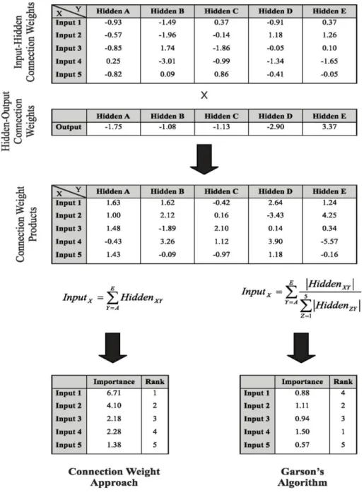
2.5.3 Connection weight approach

Calculates the product of the raw input-hidden and hidden-output connection weights

between each input neuron and output neuron and sums the products across all hidden

neurons (Olden and Jackson, 2002b).

2.5.4 Garson’s algorithm

Partitions hidden-output connection weights into components associated with each

20

Figure 2.4 Steps for connection weight approach and Garson’s algorithm (Olden, Joy and Death, 2004)

Sensitivity analysis is performed for choice of important input variables. Different

methodologies have been recommended to select the important input variables. Goh (1994) and Shahin et al. (2002) have used Garson‟s algorithm (Garson, 1991) in which the input hidden and hidden output weights of trained ANN model are segregated and the absolute

21

example have been presented in Goh (1994). It does not provide evidence on the effect of

input variables in terms of direct or inverse relation to the output. Olden et al. (2004)

suggested a connection weight approach based on the Neural Interpretation Diagram (NID),

in which the actual values of input hidden and hidden output weights are taken. It sums the

products across all the hidden neurons, which is defined as Si. The relative inputs are

corresponding to absolute Si values, where the most important input corresponds to highest Si

22

CHAPTER 3

PREDICTION OF COMPACTION PARAMETERS OF SANDY SOIL

3.1 Introduction

Compacted soils are used in many projects such as highway embankments, railway

subgrades, airfield pavements, earth dams and landfill liners. The granular materials are

generally used as fill material in earth work. In the field, soils are usually compacted using

rollers and other various equipments. To evaluate compaction in the field, laboratory

compaction parameters are required using the Standard Proctor and Modified Proctor

compaction which requires large efforts and time. A standard amount of compactive effort is

applied to produce soil density with which site values can be compared. The compaction

parameters of soils are influenced by many factors such as water content, compactive effort,

and index properties. For a certain compactive effort, a typical compaction curve that relates

the water content of the soil to its dry unit weight is usually obtained. The most important

point on the compaction curve is the optimum compaction point in which two important

parameters, maximum dry unit weight (MDD) and optimum water content (OMC), are

obtained, and they represent compaction behavior.

In recent years attempts have been made to correlate Index properties of soil and

gradation to obtain MDD and OMC of compacted sandy soils. Several researches have been

done to correlate compaction parameters with index properties of fine-grained soils (Wang

and Huang1984; Blotz et al.1999; Nagaraj et al. 2006; Sivrikaya et al. 2008; Sivrikaya 2008).

On the other hand, prediction models of coarse-grained soils are rare (Korfiatis and

Manikopoulos 1982; Omar et al. 2003). In recent years, Artificial Intelligence (AI) has been

applied successfully to several problems in geotechnical engineering. Several soft-computing

methods like Artificial Neural Network (ANN), Support Vector Machine (SVM), Genetic

23

Multivariate Adaptive Regression Splines (MARS) are continuously used in modeling of

geotechnical problems. These techniques have been used for predicting the bearing capacity

of piles, permeability of compacted clay liners, settlement prediction of shallow foundations

on granular soils, swelling pressures of soil, compaction parameters of soils, slope reliability

analysis, ultimate capacity of driven piles in cohesionless soils, OCR prediction of clay.

This study investigates the capability of ANN, MARS and LSSVM for determination

of compaction parameters of coarse-grained soils with an emphasis on the influence of soil

properties and compaction effort. MARS is a flexible, more accurate, and faster simulation

method for both regression and classification problems (Friedman, 1991). Different models

has been developed and observed that MARS gives a better predictability as compared to

regression equation and other non-linear models from ANN and MARS.

The laboratory experiment was conducted by Mujtaba et al. (2013) for the

determination of compaction parameters, grain size distribution and Index properties of sandy

soil. The compaction parameters were determined at different compaction energy (CE) level (592 kN-m/m3 & 2696 kN-m/m3) and performing regression analysis, the potential input parameters were identified which affect the output parameters. Based on the analysis a

regression model equation was developed for MDD and OMC. The model equations were as

follows: ) log( 153 . 0 ) log( 193 . 0 67 . 1 (%) ) log( 2 . 10 ) log( 51 . 1 ) log( 49 . 4 ) / ( 3 CE Cu OMC CE C m kN MDD _u       _(3.1)

where Cu = coefficient of uniformity

From the cross-correlation matrix, it is observed that two other parameters also affect

the compaction parameters i.e. fines (%) and Sand (%) along with Cu and CE. In the present

study, two models were taken into consideration consisting of the index properties and

24

Model – I Cu, CE

Model – II Fines (%), Sand (%), Cu, CE

Model-III: Fines (%), Sand (%), D50, Cu, CE

The data available in literature (Mujtaba et al., 2013) are taken with input and output

parameters. The total number of data points considered is 220 out of which 160 are taken for

training and 60 are taken for testing. Some of the data base of the experiment has been shown

in Table 3.1 and the maximum, minimum, average, and standard deviation for the data used

are shown in Table 3.2 and it can be seen that it covers a wide range of values. The successful

application of a method depends upon the identification of suitable input parameters. Table

3.2 shows the cross correlation between the inputs and output; it can be seen that fines (%),

sand (%), D50, Cu and CE are found to be important input parameters for predicting MDD and

OMC.

Table 3.1. some of the compaction of test data and index properties of soil

Sample No. Gravel (%) Sand (%) Fines (%) D60 (mm) D50 (mm) D30 (mm) D10 (mm) MDD (m) (kN/m3) OMC (m) (%) MDD (s) (kN/m3) OMC (s) (%) 1 0 67 33 0.12 0.1 0.06 0.0319 18.2 11 17.2 14 2 3 64 33 0.15 0.11 0.06 0.014 20.1 9 19.1 12 3 0 91 9 0.11 0.1 0.09 0.075 16.3 13 15.4 16.5 4 0 92 8 0.11 0.1 0.09 0.075 16.0 13.5 15.2 16.5 5 2 82 16 0.2 0.17 0.1 0.06 17.9 12 17.0 16 6 0 84 16 0.2 0.17 0.1 0.04 18.1 11.5 17.1 15 7 4 68 28 0.27 0.2 0.08 0.024 20.0 8 18.9 11 8 0 70 30 0.21 0.19 0.08 0.02 20.0 9 18.9 11.5 9 2 70 28 0.22 0.19 0.08 0.019 20.4 9.5 19.3 12 10 0 57 43 0.16 0.1 0.055 0.021 20.0 9.5 18.9 12 11 0 96 4 0.12 0.11 0.1 0.08 16.3 14.5 15.4 18 12 0 94 6 0.11 0.1 0.09 0.08 16.2 15.5 15.4 18 13 0 92 8 0.7 0.58 0.27 0.085 19.8 11 18.8 12.5 14 0 92 8 0.17 0.14 0.1 0.075 16.3 14 15.6 17.5 15 3 52 45 0.16 0.09 0.04 0.017 20.4 9.5 19.5 10.5 16 2 79 19 0.21 0.19 0.1 0.05 18.2 10 17.3 12.5 17 2 72 26 0.2 0.18 0.09 0.045 18.9 11 18.1 14 18 0 83 17 0.21 0.2 0.15 0.05 17.9 11 17.0 14 19 0 54 46 0.15 0.095 0.058 0.027 19.0 9 18.1 12 20 0 71 29 0.2 0.16 0.08 0.021 19.2 9 18.2 12 21 2 74 24 0.2 0.16 0.09 0.038 18.5 9 17.6 11 22 3 77 20 0.195 0.15 0.092 0.05 17.6 11 16.7 14 23 2 60 38 0.15 0.11 0.06 0.026 18.8 9.5 17.9 12

25 24 5 50 45 0.12 0.09 0.05 0.026 19.0 9 18.1 11 25 0 83 17 0.21 0.19 0.11 0.05 17.4 11.5 16.6 15 26 0 86 14 0.27 0.21 0.17 0.051 17.9 13 16.8 16 27 0 94 6 0.21 0.2 0.14 0.08 17.7 12 16.7 15.0 28 0 95 5 0.28 0.21 0.18 0.09 17.4 12 16.6 15.0 29 2 90 8 0.6 0.425 0.21 0.083 19.4 9.5 18.4 12 30 2 96 2 0.4 0.3 0.21 0.11 18.7 10.5 17.8 13 31 1 97 2 0.55 0.4 0.22 0.15 18.5 12 17.6 15.0 32 1 84 15 0.25 0.19 0.1 0.06 18.7 9.5 17.8 12 33 1 97 2 0.43 0.35 0.21 0.14 18.4 10.5 17.4 13 34 2 95 3 0.9 0.78 0.4 0.19 18.3 11 17.4 14 35 0 94 6 0.19 0.15 0.11 0.08 17.3 12.5 16.4 15.5 36 0 100 0 0.28 0.25 0.19 0.14 17.5 11 16.6 14 37 1 96 3 0.425 0.32 0.2 0.1 18.9 10 18.1 12.5 38 1 96 3 0.26 0.2 0.15 0.09 18.2 12.5 17.3 16 39 0 100 0 0.8 0.6 0.32 0.15 19.5 8.5 18.5 11 40 0 95 5 0.24 0.2 0.13 0.082 18.3 10 17.3 13 41 2 95 3 0.39 0.3 0.18 0.1 17.9 11 16.9 14.5 42 1 96 3 0.4 0.3 0.19 0.1 17.9 10 17.0 13 43 2 96 2 0.5 0.39 0.21 0.12 17.9 12 17.0 15.0 44 2 93 5 0.28 0.2 0.14 0.09 17.3 10 16.4 13 45 2 96 2 0.5 0.37 0.21 0.15 17.8 9.5 16.8 12 46 1 95 4 0.29 0.21 0.15 0.09 17.3 11 16.4 14.5 47 2 94 4 0.31 0.29 0.18 0.1 17.4 12 16.6 15.0 48 0 95 5 0.21 0.19 0.13 0.081 17.4 13 16.5 16.5 49 2 96 2 0.7 0.5 0.35 0.17 18.3 10.5 17.4 13.5 50 2 96 2 0.425 0.31 0.21 0.15 17.9 11 17.0 14 51 1 93 6 0.28 0.2 0.14 0.08 17.9 9.5 17.1 12 52 1 94 5 0.3 0.23 0.16 0.09 17.7 10 16.7 12.5 53 1 93 6 0.3 0.21 0.15 0.085 17.7 10 16.7 12.5 54 0 91 9 1 0.75 0.3 0.085 20.7 9 19.6 11.5 55 0 100 0 0.2 0.19 0.12 0.09 16.2 15.5 15.2 18.5 56 0 95 5 0.22 0.19 0.12 0.08 16.7 14.5 15.5 18 57 0 91 9 0.28 0.2 0.12 0.079 17.5 9.5 16.7 12 58 0 86 14 0.3 0.2 0.11 0.06 18.5 10 17.3 12 59 0 62 38 0.2 0.14 0.054 0.02 19.2 9 18.1 11.5 60 0 98 2 0.201 0.18 0.11 0.09 16.7 13 15.9 16 61 0 97 3 0.2 0.19 0.12 0.085 16.9 12 16.0 15 62 1 97 2 0.7 0.48 0.21 0.1 18.9 11 18.0 14 63 0 71 29 0.25 0.19 0.08 0.03 19.2 9.5 18.2 11.5 64 1 83 16 0.3 0.21 0.11 0.05 19.7 9 18.7 12 65 0 64 36 0.3 0.19 0.062 0.03 20.0 9 19.0 11.5 66 5 87 8 1 0.8 0.425 0.09 20.2 8.5 19.3 12 67 1 95 4 1 0.8 0.425 0.11 20.0 10.0 19.0 12.5 68 1 68 31 0.19 0.14 0.075 0.033 18.6 10.5 17.6 13 69 0 84 16 0.21 0.2 0.15 0.05 19.2 9.5 18.1 12 70 0 83 17 0.18 0.17 0.1 0.07 16.9 11.5 15.6 14.5 71 0 86 14 0.23 0.21 0.16 0.07 16.8 11 15.9 13.5 72 0 94 6 0.21 0.2 0.11 0.08 16.6 13.5 15.7 17 73 0 95 5 0.29 0.21 0.18 0.09 16.7 10.5 15.9 13.5 74 2 90 8 0.6 0.425 0.2 0.08 18.6 9 17.6 11.5 75 2 96 2 0.4 0.3 0.2 0.13 18.2 10.5 17.3 13.5 76 1 97 2 0.57 0.4 0.22 0.15 18.4 11 17.4 13.5 77 1 84 15 0.24 0.19 0.1 0.06 17.3 11.5 16.4 14.5

26

78 1 97 2 0.44 0.35 0.2 0.15 18.3 10.5 17.4 13 79 2 95 3 0.85 0.7 0.4 0.21 17.3 9 16.3 11 80 0 94 6 0.2 0.15 0.1 0.08 17.5 10.5 16.7 13

m: modified Proctor test, s: standard Proctor test

Table 3.2 Summary of Statistical values of input and output parameters

Fines (%) Sand (%) D50 Cu CE MDD OMC

Maximum 100 46 0.8 11.765 2696 20.75 18.50 Minimum 50 0 0.09 1.375 592 15.17 8.00 Average 88.5 10.44 0.274 4.55 1644 17.62 12.19 Standard Deviation 11.63 11.48 0.166 2.51 1054.4 1.183 2.18

Table 3.3 Cross correlation between the inputs and output

Sand (%) Fines (%) D50 Cu CE MDD OMC

(%) Sand (%) 1 Fines (%) -0.995 1 D50 0.40154 -0.4269 1 Cu -0.556 0.5448 0.324 1 CE 0 0 0 0 1 MDD -0.447 0.431 0.332 0.774 0.42 1 OMC (%) 0.309 -0.284 -0.205 -0.455 -0.643 -0.76 1 3.2 Database preprocessing

The database has been normalized between 0 to 1 for LS-SVM model by using the

formula: min max min X X X X X_n   

For ANN and MARS modeling, the actual database has been used.

3.3 Developed model equations

3.3.1 ANN model equation

In the neural network model, Levenberg-Marquartd back-propagation has been used

for minimization of error for both the models. The hyperbolic tangent sigmoid transfer

function for input-hidden layer and linear transfer function for hidden layer-output layer has

27

The final ANN model equation can be given as follows:

A1 = -11.167 a - 13.829 b - 99.4175 Cu + 0.00034 CE + 1363.383

A2 = 3.808 a - 3.126 b - 7.536 Cu - 0.00003331 CE -328.6133

A3 = 0.03571 a + 0.0228 b - 0.3913 Cu - 0.000068 CE -1.6421

A4 = 51.961 a + 39.188 b + 32.941 Cu - 2.336 CE -1.2856

MDD = -0.8841 tanh(A1) + 0.8931 tanh(A2) - 4.8144 tanh(A3) - 0.8341 tanh(A4) + 20.293

(3.2) A1 = -11.2872 a + 10.0223 b- 2.7313 Cu - 0.3716 CE + 28.6707

A2 = 1.2647 a + 1.1810 b - 2.5487 Cu - 0.0005 CE - 118.8911

A3 = -0.0542 a - 0.0574 b + 0.0154 Cu + 0.0149 CE - 37.0904

A4 = 3.2903a + 2.9314 b - 3.6901 Cu + 0.0005 CE - 295.7113

OMC = -3.1872 tanh(A1) + 3.8722 tanh(A2) -26.9176 tanh(A3) + 1.4801 tanh(A4) +

11.7996 (3.3)

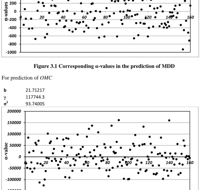
3.3.2 LS-SVM model equation

For the LS-SVM model, Radial basis kernel function has been used for transformation

of the inputs in the prediction of MDD and OMC. The optimum values of bias, regularization

parameter and with of radial basis function is given below and the values for Lagrange

multiplier for all the inputs have been represented in Figure 3.1 and 3.2:

For prediction of MDD

γ 901.8988

b 1.967575

σ2

28

Figure 3.1 Corresponding α-values in the prediction of MDD

For prediction of OMC

b 21.71217

γ 117744.3

σ2

93.74005

Figure 3.2 Corresponding α-values in the prediction of OMC

3.3.3 MARS model equation

For developing the MARS, 19 and 16 basis functions have been introduced in forward

phase for modeling MDD & OMC respectively and in backward elimination phase, 6 and 5

basis functions have been removed from the MARS model. So, the final MARS contains 13

and 11 basis functions respectively for MDD and OMC. The optimal MARS model is given

below -1000 -800 -600 -400 -200 0 200 400 600 800 1000 0 20 40 60 80 100 120 140 160 α -v al u e s -150000 -100000 -50000 0 50000 100000 150000 200000 0 20 40 60 80 100 120 140 160 α -valu e

29 Table 3.4 Basis functions of MARS model Basis Functions MDD OMC BF1 BF2 BF3 BF4 BF5 BF6 BF7 BF8 BF9 BF10 BF11 BF12 BF13 max(0, Cu -5.33) max(0, 5.33 -Cu) max(0, 2700 -CE) max(0, b -5) max(0, 5 -b) BF5 × max(0, Cu -2.93) BF5 × max(0, 2.93 -Cu) BF1 × max(0, b -38) BF5 × max(0, a -94) BF5 × max(0, 94 -a) BF9 × max(0, 2.23 -Cu) BF4 × max(0, Cu -4.17) BF4 × max(0, 4.17 -Cu) max(0, CE -592) max(0, Cu -3.29) × max(0, b -2) max(0, Cu -3.29) × max(0, 2 -b) BF2 × max(0, Cu -3.53) BF2 × max(0, 3.53 -Cu) max(0, Cu -3.29) × max(0, Cu -3.64) max(0, Cu -3.29) × max(0, 3.64 -Cu) max(0, 3.29 -Cu) × max(0, b -2) max(0, 3.29 -Cu) × max(0, 2 -b) max(0, 3.29 -Cu) × max(0, a -95) max(0, 3.29 -Cu) × max(0, 95 -a) MDD = 18.2 + 0.438 BF1 - 0.377 BF2 - 0.000473 BF3 + 0.0327 BF4 + 0.19 BF5 - 0.0857 BF6 - 0.766 BF7 + 0.0411 BF8 + 0.0461 BF9 + 0.603 BF10 + 0.173 BF11 - 0.00906 BF12 - 0.0478 BF13 (3.4) OMC = 13.6 - 0.00131 BF1 - 0.0203 BF2 - 0.516 BF3 + 0.00271 BF4 + 21.7 BF5 - 0.0304 BF6 - 41.2 BF7 + 0.743 BF8 - 1.37 BF9 + 0.592 BF10 - 0.858 BF11 (3.5)

Then all the models for the prediction of Maximum Dry density (MDD) were

compared as per Root Mean Square Error (RMSE) and Mean Absolute Percentage Error

(MAPE).

3.4 Performance comparison among all the models

The error criteria like MAE, MAPE, RMSE, R and R2 for all the models in the prediction of MDD and OMC are presented in Table 3.5 and 3.6 respectively. The results of MARS have been compared with ANN and LS-SVM model developed. The comparisons

have been done in terms of Mean Absolute Percentage Error (MAPE), and Root Mean Square

Error (RMSE). Figure 3.7 and 3.8 depict the bar chart of MAPE and RMSE for training

dataset, respectively. It is observed from Figure 3.7 and 3.8 that the developed MARS

30

entire dataset, but splits the whole model into linear regions and produces discrete functions

for each of the produced linear area. Researches emphasized that regression equations

obtained by the MARS technique make robust and coherent parameter valuations. Figure 3.5

and 3.6 represents the actual versus predicted value of MDD and OMC respectively and Figure 3.3 and 3.4 presents the performance of MARS model in the prediction of MDD and

OMC respectively.

Table 3.5 Results of Different Models for Prediction of MDD of sandy soil

Model Model

Inputs MAE RMSE MAPE

Correlation coefficient ( R ) Coefficient of determination (R2) Mujtaba et al. (2013) Cu, CE Regression 0.432 0.512 2.46 0.9 0.81 Model I Cu, CE ANN Training 0.436 0.52 2.48 0.9 0.81 Testing 0.4 0.49 2.31 0.9 0.81 SVM Training 0.41 0.494 2.35 0.911 0.829 Testing 0.45 0.54 2.526 0.89 0.767 MARS Training 0.35 0.43 2 0.936 0.875 Testing 0.353 0.42 2.2 0.923 0.853 Model II a, b, Cu, CE ANN Training 0.335 0.43 1.89 0.935 0.872 Testing 0.35 0.43 2.04 0.926 0.858 SVM Training 0.322 0.4 1.845 0.934 0.871 Testing 0.415 0.486 2.38 0.928 0.853 MARS Training 0.32 0.39 1.82 0.94 0.887 Testing 0.33 0.4 1.91 0.937 0.877 Model III a, b, D50, Cu, CE ANN Training 0.35 0.44 2 0.935 0.87 Testing 0.39 0.47 2.24 0.92 0.815 SVM Training 0.36 0.45 2.06 0.92 0.848 Testing 0.369 0.462 2.11 0.93 0.86 MARS Training 0.314 0.4 1.79 0.93 0.877 Testing 0.3 0.41 1.72 0.94 0.89 a : Sand (%), b : Fines (%)

31

Table 3.6 Results of Different Models for Prediction of OMC of sandy soil

Model Model

Inputs MAE RMSE MAPE

Correlation coefficient ( R ) Coefficient of determination (R2) Mujtaba et al. (2013) Cu, CE Regression 0.963 1.21 7.85 0.83 0.69 Model I Cu, CE ANN Training 0.91 1.18 7.62 0.855 0.71 Testing 1.05 1.2 8.9 0.857 0.687 SVM Training 0.94 1.17 7.72 0.84 0.705 Testing 0.931 1.174 7.44 0.85 0.719 MARS Training 0.81 0.98 6.75 0.89 0.79 Testing 0.756 0.93 6.24 0.91 0.825 Model II a, b, Cu, CE ANN Training 0.856 1.08 6.93 0.874 0.76 Testing 0.851 1.05 7.18 0.871 0.745 SVM Training 0.865 1.09 7.06 0.867 0.751 Testing 0.91 1.12 7.606 0.855 0.72 MARS Training 0.74 0.94 6.17 0.903 0.815 Testing 0.72 0.95 5.97 0.896 0.8 Model III a, b, D50, Cu, CE ANN Training 0.845 1.05 6.92 0.88 0.77 Testing 0.82 1.01 6.93 0.879 0.764 SVM Training 0.83 1.08 6.71 0.87 0.758 Testing 0.859 1.05 7.11 0.868 0.753 MARS Training 0.75 0.934 6.15 0.907 0.822 Testing 0.77 0.93 6.52 0.9 0.8

Figure 3.3 Performances of MARS model for prediction of MDD

14 15 16 17 18 19 20 21 22 14 16 18 20 22 P red ict ed M D D f rom M A RS (kN /m 3) Observed MDD (kN/m3₎ Training dataset ( R = 0.94 ) Testing dataset ( R = 0.937 )