Probabilistic Argumentation: An Equational Approach

(1)

c

2015 Springer Basel

1661-8297/15/030345-38,published onlineApril 25, 2015

DOI 10.1007/s11787-015-0120-1 Logica Universalis

Probabilistic Argumentation: An Equational

Approach

D. M. Gabbay and O. Rodrigues

Abstract.There is a generic way to add any new feature to a system. It involves (1) identifying the basic units which build up the system and (2) introducing the new feature to each of these basic units. In the case where the system isargumentationand the feature is probabilistic we have the following. The basic units are: (a) the nature of the arguments involved; (b) the membership relation in the setSof arguments; (c) the attack rela-tion; and (d) the choice of extensions. Generically to add a new aspect (probabilistic, or fuzzy, or temporal, etc) to an argumentation network

S, Rcan be done by adding this feature to each component (a–d). This is a brute-force method and may yield a non-intuitive or meaningful result. A better way is to meaningfully translate the object system into another target system which does have the aspect required and then let the target system endow the aspect on the initial system. In our case we translate argumentation into classical propositional logic and get probabilistic argu-mentation from the translation. Of course what we get depends on how we translate. In fact, in this paper we introduce probabilistic semantics to abstract argumentation theory based on the equational approach to argumentation networks. We then compare our semantics with existing proposals in the literature including the approaches by M. Thimm and by A. Hunter. Our methodology in general is discussed in the conclusion. Mathematics Subject Classification. Primary 68T27; Secondary 60B99, 68T30.

Keywords.Argumentation, probability theory, numerical methods.

1. Introduction

The objective of this paper is to provide some orientation to underpin prob-abilistic semantics for abstract argumentation. We feel that a properly devel-oped probabilistic argumentation framework cannot be obtained by simply imposing an arbitrary probability distribution on the components of an argu-mentation system that does not agree with the dynamic aspects of these net-works. We need to ﬁnd a probability distribution that is compatible with their underlying motivation.

(2)

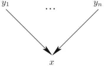
y1 yn

x

Figure 1. _{Basic attack formation in an argumentation network}

We shall use the methodology of “Logic by Translation”, which works as follows: Given a new area for which we want to study certain aspect properties AP, we translate this area to classical logic, study AP in classical logic and then translate back and evaluate what we have obtained.

Let us start by looking at interpretations of an abstract argumentation networkS, R,S=∅,R⊆S×S, into logics which already have probabilistic versions. This way we can import the probability aspect from there and it will have a meaning. We begin with translating abstract argumentation frames into classical propositional logic. In the abstract form, the elements of S are just atoms waiting to be instantiated as arguments coming from another applica-tion system.Rmay be deﬁned using the source application system or may rep-resent additional constraints. At any rate, in this abstract form,Sis just a set of atoms and all we have about it isR. In translatingS, Rinto classical propo-sitional logic, we viewS as a set of atomic propositions and we useRto gener-ate a classical theory Δ_{S, R}. Consider Fig.1, which describes the basic attack formation of all the attackersAtt(x) ={y ∈S |(y, x)∈R}={y1, . . . , yn} of

the nodexin a networkS, R.

The essential logic translation of the attack on each nodex is given by (E1) below, where x, yi are propositional symbols representing the elements

x, yi∈S:

x↔

i

¬yi (E1)

SoS, Rcorresponds to a classicalpropositionaltheory Δ_{S, R}={x↔

i¬yi|x∈S}.1 Note that in classical logic, this theory may be inconsistent and have no models. For example, if S contains a single node x and R is

{(x, x)}, i.e., the network has a single self-attacking node, then the associated theory is{x↔ ¬x}, which has no model. For this reason it is convenient to regard these theories as theories of Kleene three-valued logic, with values in

1_{If there is a logical relationship between the arguments of}_S_{that can be captured by}

formu-lae, then we can alternatively instantiatex−→ϕx, giving Δ_{S, R}={ϕx↔_i¬ϕy|x, y∈ S}.

(3)

{0,1

2,1}. In this 3-valued semantics, a valuation would satisfyx↔ ¬xif and

only if it gives the value 1₂ tox.2

If we consider theequational approach[5], then we can write

x=

i

¬yi (E2)

where (E2) is a numerical equation over the real interval [0,1], with conjunction and negation interpreted as numerical functions expressing the correspondence of the values of the two sides.

A complete extension ofS, Ris a solution to the equations of the form of (E2) when they are viewed as a set of Boolean equations in Kleene’s 3-valued logic with values0,1₂,1, where

x= 0 means that x=out(at least one attackeryi=in) (1)

x= 1 means that x=in(all attackersyi =out) (2)

x= 1

2 means that x=und (no attackeryi =in and at least (3) one attackeryj=und)

The acceptability semantics above can be re-written in terms of the semantics of Kleene’s logic as

v(x) = min{1−v(yi)} which in equational form can be simpliﬁed to

x= 1−max{yi} (E2*)

The reader should note that we actually solve the equations over the unit interval [0,1] and project onto Kleene’s 3-valued logic by letting

x= 0 meanx=out (at least one attackeryi=in) 0< x <1 meanx=und(no attackeryi=inand at least

one attackeryj=und)

x= 1 meanx=in (all attackersyi=out)

Now there are probabilistic approaches to two-valued classical logic. The simplest two methods are described in Gabbay’s bookLogic for Artificial Intel-ligence and Information Technology[4]. Our idea is to bring the probabilistic approach through the above translation into argumentation theory.

Let us start with a description of the probabilistic approaches to classical propositional logic.

Method 1: SyntacticImpose probabilityP(q) on the atomsq of the lan-guage and propagate this probability to arbitrary well-formed formulas (wﬀs). So ifϕ(q1, . . . , qm) is built up from the atomsq1, . . . , qm, we can calculateP(ϕ)

if we knowP(qi),i= 1, . . . , m.

2_{In Kleene’s logic, one can interpret}_¬_{as complement to 1;}_∧_{as min; and}_∨_{as max. Thus,}

if the values ofA, Barev(A), v(B), thenv(¬A) = 1−v(A),v(A∧B) = min(v(A), v(B)) andv(A∨B) = max(v(A), v(B)).

(4)

Method 2: SemanticImpose probability on the models of the language of

{q1, . . . , qm}. The totality of models is the spaceW of all{0,1}-vectors in 2m.

We give valuesP(ε), for anyε∈2m, with the restriction that Σ_ε_∈₂mP(ε) = 1. The probability of any wﬀϕis then

P(ϕ) = ΣεϕP(ε) (P1)

The motivation for the syntactical Method 1 is that the atoms{q1, . . . ,

qm} are all independent. So for example, the date of birth of a person (p) is independent of whether it is going to rain heavily on that person’s 21st birthday (q). However, if we want to hold a birthday partyrin the garden on the 21st birthday, then we have thatqattacksr.

If, on the other hand, we have:

a= John comes to the party

b= Mary comes to the party

thenaandbmay be dependent, especially if some relationship exists between John and Mary. We may decide that the probability of a∧b is 0, but the probabilities of¬a∧band ofa∧ ¬bare 1

4 each and the probability of¬a∧ ¬b

is 1₂. Assigning probability in this way depends on the likelihood we attach to a particular situation (model). This is the semantic approach.

Example1.1shows that these two methods are orthogonal.

Example 1.1. What can Δ_{S, R} mean in classical logic? It is a generalisation of the “Liar’s paradox”.xattacking itself is likexsaying “I am lying”:x= if and only ifx=⊥. Figure1representsyi sayingxis a lie. Δ_{S, R}represents a system of lying accusations: acommunity liar paradox.

Similarly, S can represent people possibly invited to a birthday party.

y→xmeansy saying “if I come,xcannot come”. So Fig.1 is saying “invite

xif and only if you do not invite any of the yi”.

Suppose we instantiatex−→ϕx. Then we must have

P(ϕx) =P i ¬ϕyi .

However, there may be also a connection betweenϕxand someϕyk, e.g.,

ϕxϕyk. This will impose further restrictions onP(ϕx) and P(ϕyk), and it may be the case that no such probability function exists.

Remark 1.2. The two approaches are of course, connected. If we are given a probability on eachqi, then we get probability on eachε∈2mby letting

P(ε) = Π_ε_qP(q)×Π_ε_¬_q(1−P(q)) (P2) Theqi’s are considered independent, so the probability ofi±qi is the product of the probabilities

P(_i±qi) = ΠiP(±qi)

whereP(¬qi) = 1−P(qi) and the probability ofA∨B is

(5)

when¬(A∧B), as is the case with disjuncts in a disjunctive normal form. So, for example

P((a∧b)∨(a∧ ¬b)) =P(a∧b) +P(a∧ ¬b) =P(a)P(b) +P(a)(1−P(b)) =P(a)(P(b) + 1−P(b)) =P(a).

2. The Syntactical Approach (Method 1)

Let us investigate the use of the syntactical approach.

Let S, R be an argumentation network. In the equational approach, according to the syntactical Method 1, we assign probabilities to all the atoms and are required to solve the Eq. (E3) below for eachx, whereAtt(x) ={yi} andxand allyi are numbers in [0,1]:

P(x) =P i ¬yi , (E3)

Since in Method 1, all atoms are independent, (E3) is equivalent to (E3*):

P(x) = Π_i(1−P(yi)). (E3*) Such equations always have a solution.

Let us check whether this makes sense. Let us try to identify the argument

xequationally with its probability, namely we let P(x) =x. Ifx=in, letP(x) = 1

Ifx=out, letP(x) = 0. Ifx=und, let 0< P(x)<1

to be determined by the solution to the equations.

Equation (E3*) becomes, underP(x) =x, the following:

x= Π(1−yi) forx∈S. (E4) This is the Eqinv equation in the equational approach (see [5]).

The following deﬁnition will be useful in the interpretation of values from [0,1] and their counterparts in Caminada’s labelling functions.

Definition 2.1. A valuation functionf can be mapped into a labelling function

λ(f) as follows.

f(x) = 1 → λ(f)(x) =in

f(x) = 0 → λ(f)(x) =out

f(x)∈(0,1) → λ(f)(x) =und

(6)

a b

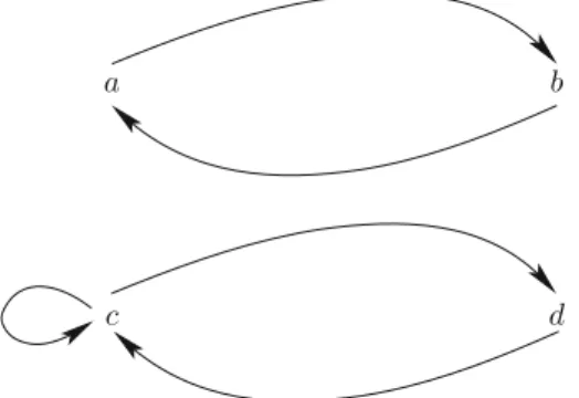
Figure 2. _{A sample argumentation network having a} com-plete extension that cannot be found via Equations (E4)

Theorem 2.2. Let fbe a solution to Eq. (E4). Then λ(f)defined according to Definition 2.1 is a legal Caminada labelling (see [1]) and leads to a complete extension.

Theorem 2.3. Letλ0be a legal Caminada labelling leading to a preferred

exten-sion. Then there exists a solutionf0, such that λ0=λ(f0).

Remark 2.4. There are (complete) extensionsλsuch that there does not exist anf withλ =λ(f).

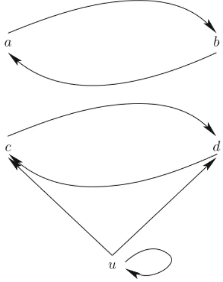
For example, in Fig.2, the extensiona=b=undcannot be obtained by anyf. Onlyb=in,a=outcan be obtained as a solution to Eq. (E4).3 Example2.5. LetS, Rbe given and letλbe a complete extension which is not preferred! The reason thatλis not preferred, is that we have by deﬁnition, a

λ1extendingλ, which gives more{in,out}values to pointsz, for whichλgives

the valueund. Therefore, we can prevent the existence of such an extensionλ1,

if we force such pointszto be undecided. This we do by attacking such points

z by a new self-attacking point u. The construction is therefore as follows. We are given S, R and a complete extension λ, which is not preferred. We now construct a newS, Rwhich is dependent onλ. ConsiderS, Rwhere

S=S∪ {u}, whereu∈S, is a new point. LetR be

R=R∪ {(u, u)} ∪ {(u, v)|v∈S andλ(v) =und}.

Then λ = λ ∪ {(u,und)} is a preferred extension of S, R and can therefore be obtained from a functionf using the Eq. (E4).

Let us see what the construction above does to our example in Fig. 2, and let us look at the extensionλ(a) =λ(b) =und.

Consider the network in Fig.3. Its Eq. (E4) are: 1. u= 1−u

2. a= (1−u)(1−a)(1−b) 3. b= (1−u)(1−a) From (1) we getu=1

2. So we have:

3_{The equations are}

1. a= (1−a)×(1−b) 2. b= 1−a.

From the above two equations we get 3. a= (1−a)×a

(7)

u

a b

Figure 3. _{The network of Fig.} ₂ _{with an extra undecided} nodeuattacking all nodes

2. a=1 2(1−a)(1−b) 3. b= 1₂(1−a) 1−b= 1−1 2(1−a) = 2−1+₂ a = 1+a 2

therefore substituting in (1) we get

a= 1₂(1−a)(1+₂a) = 1 4(1−a2) 4a+a2₋_{1 = 0} (a+ 2)2₋₄₋_{1 = 0} (a+ 2)2_{= 5} a=√5−2≈0.236 b= 1₂(1−a) = 1 2(1− √ 5 + 2) = 3−₂√5 ≈0.382.

The extension of the network isa=b=und.

Summary of the results so far for the syntactical probabilistic method. Given an argumentation network S, R, we can ﬁnd all Method 1 complete probabilistic extensions for it by solving all Eq_inv equations. Such complete probabilistic extensions will also be complete extensions in the traditional sense (i.e., Dung’s), which will also include all preferred extensions (Theorems 2.2 and2.3).4

4_{Note that in traditional Dung semantics a preferred extension}_E _{is maximal in the sense}

that there is no extensionE such that

1. Ifxis consideredin(resp.out) byEthenxis also consideredin(resp.out) byE. 2. There exists at least one node consideredin(resp.out) byEand consideredundbyE. The above deﬁnition holds for numerical or probabilistic semantics, where the value 1 (resp. 0) is understood asin(resp.out) and values in (0,1) are understood asund.

(8)

However, not all complete extensions can be obtained in this manner (i.e., by Method 1, see Remark2.4and compare with Example3.6).

We can, nevertheless, for any complete extension E which cannot be obtained by Method 1, obtain it from the solutions of the equations generated for a larger networkS, Ras shown in Example2.5.

We shall say more about this in a later section.

Remark 2.6. Evaluation of the results so far for the syntactical probabilistic method.

1. We discovered a formal mathematical connection between the syntactical probabilistic approach (Method 1) and the Equational Eqinv approach.

Is this just a formal similarity or is there also a conceptual connection? The traditional view of an abstract argumentation frameS, R, is that the arguments are abstract, some of them abstractly attack each other. We do not know the reason, but we seek complete extensions of arguments that can co-exist (i.e., being attack-free), and that protect themselves. The equational approach is an equational way of ﬁnding such extensions. Each solutionfto the equations give rise to a complete exten-sion. The numbers we get from such solutionsfof the equational approach can be interpreted as giving the degree of being in the complete extension (associated withf) or being out of it.

Due to the mathematical similarity with the probability approach, these numbers are now interpreted as probabilities.

To what extent is this justiﬁed? Can we do this at all?

Let us recall the syntactical probabilistic method. We start with an abstract argumentation frameworkS, R and add the probabilityP(x) for each x ∈ S. We can interpret P(x) as the probability that x “is a player” to be considered (this is a vague statement which could mean anything but is suﬃcient for our purpose). The problem is how do we take into account the attack relation? Our choice was to require Eq. (E3). It is this choice that allowed the connection between the syntactical prob-abilistic approach and the Equational approach with Eq_inv.

So our syntactical probabilistic approach should work as follows. Let P be the independent probability on each x ∈ S. This is an arbitrary number in [0,1]. Such aP cannot be used for calculating exten-sions because it does not take into consideration the attack relationR. So modifyP to aP which does respectRvia Eq. (E3).

How do we modifyP to ﬁnd P?

Well, we can use a numerical iteration method. The details are not important here, the importance is in the idea, which can be applied to the traditional notion of extensions as well. Given S, R and an arbi-trary desired assignment E of elements that are in (and consequently also determining elements that areout) for S, thisE may not be legit-imate in taking into accountR, so we need to modify it to get the best proper extensionE nearest toE(cf. [2,6]).

(9)

So our syntactical probabilistic approach yielding a P satisfying Eq. (E3) can be interpreted as Eq_inv extensions obtained from initial values which are probabilities (as opposed to, say, initial values being a result of voting) corrected via iteration procedures usingR.

Alternatively, we can look at the Eqinvequations as a mathematical

means of ﬁnding all those syntactical probabilitiesP which respect the attack relationR [via Eq. (E3)].

Or we can see the solutions of the Eqinv as giving probabilities for

being included or excluded in the complete extension deﬁned by these solutions (as opposed to the interpretation of the degree of being in or

out).

2. The discussion in item 1. above hinged upon the choice we made to take account of R by respecting Eq. (E3). There are other alternatives for takingR into account. We can give direct, well-motivated deﬁnitions of how to propagate probabilities along attack arrows. This is similar to the well-known problem of how to propagate probabilities along proofs (provability support arrows, or modus ponens, etc). Such an analysis is required anyway for instantiated networks, for example in ASPIC+ style [10]). We shall deal with this in a subsequent paper.

3. The Semantical Approach (Method 2)

Let us now check what can be obtained if we use Method 2, i.e., giving probabil-ity to the models of the language. In this case the equation (for{yi}=Att(x)) (E3) P(x) = P(_i¬yi) still holds, but the ¬yi are not independent. So we cannot write Eq. (E3*) for them and get Eqinv. Instead we need to use the

schemaP(A∨B) =P(A) +P(B)−P(A∧B). We begin with a key lemma, which will enable us to compare later with the work of M. Thimm, see [13].

Lemma 3.1. LetS, Rbe a network and let P be a probability measure on the spaceW of all models of the language whose set of atoms is S. Forx∈S, let the following hold

P(x) =P _n i=1 ¬yi whereAtt(x) ={y1, . . . , yn}. Then we have 1. P(x)≤P(¬yi),1≤i≤n 2. P(x)≥1−Σn_i₌₁P(yi) Proof. By induction onn.

1. Ifx=¬y thenP(x) = 1−P(y) and the above holds.

2. Assume the above holds form, show form+1. Letz=_im₌₁yi, y=ym+1.

Thenx=¬z∧ ¬y.

We have by the induction hypothesis

(10)

• P(¬z)≥1−Σm_i₌₁P(yi) Consider now: P(¬z∧ ¬y) = 1−P(y∨z) = 1−(P(y) +P(z)−P(y∧z)) = 1−P(y)−P(z) +P(y∧z) = 1−P(y)−(P(z)−P(y∧z)) ButP(A∧B)≤P(B) is always true.

So

P(¬z∧ ¬y)≤1−P(y) =P(¬y) On the other hand, by our assumption

1−P(z) =P(¬z)≥1−Σm_i₌₁P(yi) So P(¬z∧ ¬y) = 1−P(y)−P(z) +P(y∧z) (1−P(z))−P(y) +P(y∧z) ≥1−ΣP(yi)−P(y) +P(y∧z) ≥1−Σm_i₌₁+1P(yi) Remark 3.2. The converse of Lemma 3.1 does not hold, as we shall see in Example3.5below.

Let us look at some examples illustrating the use of Method 2.

Example 3.3. Consider the network in Fig. 4. This ﬁgure is taken from Thimm’s “A probabilistic semantics for abstract argumentation” [13, Figure 1]. We include it here for two reasons:

1. To illustrate or probabilistic semantic approach.

2. To use it later to compare our work with Thimm’s approach.

a1 a2 a3

a4

a5

Figure 4. _Figure₁_{of “A probabilistic semantics for abstract} argumentation” [13]

(11)

Let us apply Method 2 to it and assign probabilities to the models of the propositional language with the atoms{a1, a2, a3, a4, a5}. We assignP as

follows.

P(a1∧ ¬a2∧a3∧ ¬a4∧a5) = 0.3

P(a1∧ ¬a2∧ ¬a3∧a4∧ ¬a5) = 0.45

P(¬a1∧a2∧ ¬a3∧ ¬a4∧a5) = 0.1

P(¬a1∧a2∧ ¬a3∧a4∧ ¬a5) = 0.15

P(any other conjunctive model) = 0.

Let us computeP(ai), fori= 1, . . . ,5. We have P(X) = εX P(ε). We get P(a1) = 0.3 + 0.45 = 0.75 P(a2) = 0.1 + 0.15 = 0.25 P(a3) = 0.3 P(a4) = 0.45 + 0.15 = 0.6 P(a5) = 0.3 + 0.1 = 0.4.

To be a legitimate probabilistic modelP must satisfy Eq. (E3) relating to the attack relation of Fig.4. Namely we must have

P(X) =P ⎛ ⎝ Y∈Att(X) ¬Y ⎞ ⎠ (E3) Therefore P(a1) =P(¬a2) P(a2) =P(¬a1) P(a3) =P(¬a2∧ ¬a5) P(a4) =P(¬a3∧ ¬a5) P(a5) =P(¬a4)

(12)

Let us calculate theP in the right hand side of the above equations. P(¬a2) = 1−0.25 = 0.75 P(¬a1) = 1−0.75 = 0.25 P(¬a2∧ ¬a5) = 0.45 P(¬a3∧ ¬a5) = 0.45 + 0.15 = 0.6 P(¬a4) = 0.4 We see that P(a3) = 0.3=P(¬a2∧ ¬a5) = 0.45.

Therefore this distributionP is not legitimate according to our Method 2. It does not satisfy Eq. (E3) because

P(a3)=P(¬a2∧ ¬a5)

Therefore Lemma 3.1 does not apply and indeed, condition (2) of Lemma3.1does not hold fora3. We haveP(a3) = 0.3 but 1−P(a2)−P(a5) =

0.35.

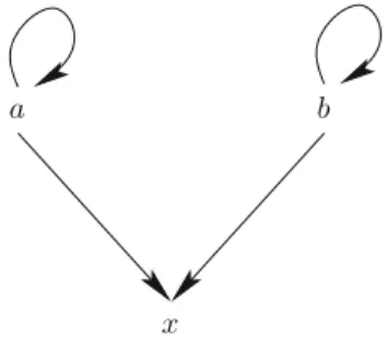
Example 3.4. Let us look at Fig. 5. This is also taken from Thimm’s paper [13, Figure 2]. It shall be used later to compare our methods with Thimm’s.

1.We use Method 2. Consider the following probability distribution on models P(a1∧ ¬a2∧ ¬a3) = 0.5 P(a1∧ ¬a2∧a3) = 0 P(a1∧a2∧ ¬a3) = 0 P(a1∧a2∧a3) = 0 P(¬a1∧a2∧a3) = 0 P(¬a1∧a2∧ ¬a3) = 0.5 a3 a2 a1

Figure 5. _Figure₂_{of “A probabilistic semantics for abstract} argumentation” [13]

(13)

P(¬a1∧ ¬a2∧a3) = 0

P(¬a1∧ ¬a2∧ ¬a3) = 0.

In this model we get

P(a1) = 0.5

P(a2) = 0.5

P(a3) = 0

Let us check whether this probability distribution satisﬁes Eq. (E3), namely P(X) =P ⎛ ⎝ Y∈Att(X) ¬Y ⎞ ⎠ (E3) We need to have P(a1) =P(¬a2) P(a2) =P(¬a1) P(a3) =P(¬a2∧ ¬a2) Indeed P(¬a1) = 1−P(a1) = 0.5 P(¬a2) = 1−P(a2) = 0.5 P(¬a1∧ ¬a2) = 0.

Thus we have a legitimate model.

2.We use Method 1. Let us use Eq_inv on this ﬁgure, namely we try and solve the equations

a1= 1−a2

a2= 1−a1

a3= (1−a1)(1−a2)

Let us use a parameter 0≤x≤1 and let

a1=x,

a2= 1−x,

(14)

The probabilities we get with parameter x as well as for x = 0.5 are given below. P(a1∧a2∧a3) =x2(1−x)2 = ₁₆1 P(a1∧a2∧ ¬a3) =x(1−x)(1−x(1−x)) = ₁₆3 P(a1∧ ¬a2∧a3) =x3(1−x) = ₁₆1 P(a1∧ ¬a2∧ ¬a3) =x2(1−x(1−x)) = ₁₆3 P(¬a1∧a2∧a3) =x(1−x)3 = ₁₆1 P(¬a1∧a2∧ ¬a3) = (1−x)2(1−x(1−x)) = ₁₆3 P(¬a1∧ ¬a2∧a3) =x2(1−x)2 = 161 P(¬a1∧ ¬a2∧ ¬a3) =x(1−x)(1−x(1−x)) = ₁₆3

If we choosex= 0.5 we get P(a1) =P(a2) = 0.5 andP(a3) = 1₄.

Example 3.5. This example shows that the converse of Lemma 3.1 does not hold. Consider the network in Fig.6.

Any legitimate probability assigned to models would be required to satisfy the following

P(a) =P(¬a∧ ¬b)

P(b) =P(¬a∧ ¬b) Case 1.Try the following probabilityP1.

P1(a∧b) =P1(a∧ ¬b) =P1(¬a∧b) =P1(¬a∧ ¬b) = 0.25.

Therefore

P1(a) = 0.5

P1(b) = 0.5

Note that we also have

P1(a) = 1 2 ≤1−P1(b) = 1 2 P1(a) = 1 2 ≤1−P1(a) = 1 2. Similarly forP1(b) by symmetry.

a b

(15)

Also P1(a) = 1 2 ≥1−P1(a)−P1(b) = 1− 1 2 − 1 2 = 0.

Thus the conditions of the conclusions of Lemma3.1 hold. However the assumptions of Lemma3.1do not hold, because

P1(a) =

1

2 =P1(¬a∧ ¬b) = 1 4.

Case 2.Let us check whether we can ﬁnd a probabilityP2which is indeed

acceptable to Method 2. Let us try with variables y, z and create equations and solve them:

P2(a∧b) =y

P2(¬a∧b) =z.

ThereforeP2(b) =y+z.

P2(¬a∧ ¬b) =y+z

and what is left is

P2(a∧ ¬b) = 1−2y−2z

but we must also have

P2(a) =P2(¬a∧ ¬b)

and hence we must have

P2(a) = 1−2y−2z+y=P2(¬a∧ ¬b) =y+z.

So we get the equation

1−2y−3z= 0 2y+ 3z= 1

y= (1−₂3z)

Since 0≤y, z≤1 soz must be less than 1₃. Let us choosez= 0.2 and soy= 0.2. We get, for example

P2(a∧b) = 0.2

P2(¬a∧b) = 0.2

P2(¬a∧ ¬b) = 0.4

(16)

We could also have chosenz= 1

3 andy= 0. This would giveP3, where

P3(a∧b) = 0 P3(¬a∧b) = 1 3 P3(¬a∧ ¬b) = 1 3 P3(a∧ ¬b) = 1 3 So we get P3(b) =P(a) = 1₃ P3(¬a∧ ¬b) =1₃.

Example 3.6. Consider the network of Fig.2. Let us try to ﬁnd a probabilistic semantics for it according to Method 2. Assume we have

P(a∧b) =x1 P(a∧ ¬b) =x2 P(¬a∧b) =x3 P(¬a∧ ¬b) = 1−x1−x2−x3. We need to satisfy P(a) =P(¬a∧ ¬b) P(b) =P(¬a)

This means we need to solve the following equations. 1. x1+x2= 1−x1−x2−x3

2. x1+x3= 1−x1−x2.

By addingx1+x2 to both sides (1) can be written as

2(x1+x2) = 1−x3,

and by swappingx3to the right and−x1−x2to the left (2) can be written as

2x1+x2= 1−x3.

Thus we get

3. 2x1+x2= 2x1+ 2x2.

Thereforex2= 0.

There remains, therefore 4. 2x1= 1−x3.

We can choose values forx3.

Sample choice 1.x3= 1, sox1= 0.

(17)

This yieldsP(a) = 0, P(b) = 1. This is also the Eq_inv solution to

b= 1−a

a= (1−a)(1−b)

Sample choice 2.x3= 1₂. Sox1= 1₄ and the probabilities are

P2(a∧b) = 1 4 P2(a∧ ¬b) = 0 P2(¬a∧b) = 1 2 P2(¬a∧ ¬b) = 1 4.

P2 is a Method 2 probability, which cannot be given by Method 1.

Sample choice 3.x3= 0. Thenx1=1₂. We get

P3(a∧b) = 1 2 P3(a∧ ¬b) = 0 P3(¬a∧b) = 0 P3(¬a∧ ¬b) = 1 2. ThereforeP3(a) =P3(b) =1₂.

Lemma 3.7. Let S, R be a network and let P be a semantic probability (Method 2) for S, R. Let x∈S and let{yi}=Att(x). Then

1. If for some yi, P(yi) = 1 thenP(x) = 0. 2. If for allyi, P(yi) = 0 thenP(x) = 1. Proof. Let us use Fig.1where {yi}=Att(x).

Case 1. Assume that P(y1) = 1. We need to show that P(x) = 0. We

have: P(x) =P i ¬yi (E3) We also have P(A) = εA P(ε) (P1) Therefore P(x) = ε_i¬yi P(ε) P(x) = ε¬y1∧nj=1¬yj P(ε) (i)

(18)

but P(y1) = εy1 P(ε) = 1 Therefore we have ε¬y1 P(ε) = 0 (ii)

From (i) and (ii) we get thatP(x) = 0.

Case 2.We assume that for all i, P(yi) = 0 and we need to show that

P(x) = 1. We have P(x) =P¬yi P(x) = 1−Pyi (iii) We also have Pyi = Σ_ε_yiP(ε) (iv)

Suppose for someε such thatε yiwe haveP(ε)>0. Butε yi impliesε yi, for somei.

Say i= 1. Thus we haveε y1 and P(y1) = 0 andP(ε)>0. This is

impossible since

P(y1) =

εy1

P(ε) (v)

Therefore for allεsuch that εyi we have thatP(ε) = 0. Therefore by (iii) and (iv) we get

P(x) = 1.

Remark 3.8. LetS, Rbe a network and letP be a semantic probability for

S, R(Method 2).

Letλbe deﬁned as follows, forx∈S.

λ(x) = ⎧ ⎪ ⎨ ⎪ ⎩ in, ifP(x) = 1 out, ifP(x) = 0 und, if 0< P(x)<1

The perceptive reader might expect us to say thatλis a legitimate Cam-inada labelling, especially in view of Lemma3.7. This is not the case as Exam-ple3.9shows.

Example 3.9. This example shows that in the probabilistic semantics it is possible to haveP(x) = 0, while for all attackersyofxwe have 0< P(y)<1. Thus the nature of the probabilistic attack is diﬀerent from the traditional Dung one. If Att(x) is the set of all attackers of xand P(_y_∈_Att₍_x₎y) = 1, then, and only thenP(x) = 0.

(19)

a b

x

Figure 7. _{A network with Method 1 and Method 2 probabilities}

Thus the attackers ofxcan attack with joint probability. The example we give is the network of Fig.7.

This has a Method 1 probability ofP1(a) = 1₂, P1(b) =1₄ andP1(x) = 1₄.

Thus for any modelm=±a∧ ±b∧xwe have

P1(m) = 1 2 × 1 2 × 1 4 = 1 16 and for any model

m₌_±_a_{∧ ± ∧ ¬}_x we have P1(m) = 1 2 × 1 2 × 3 4 = 3 16.

Figure7also has a Method 2 probability model. We can have

P2(a) =P2(b) =

1 2

P2(x) = 0.

Let us check what values to give to the models. The models are:

m1=x∧a∧b m2=x∧a∧ ¬b m3=x∧ ¬a∧b m4=x∧ ¬a∧ ¬b m5=¬x∧a∧b m6=¬x∧a∧ ¬b m7=¬x∧ ¬a∧b m8=¬x∧ ¬a∧ ¬b.

(20)

1. P2(x) = 0. This means we need to let

P2(mi) = 0, i= 1, . . . ,4. 2. P2(a) =1₂. This means we need to let

P2(m5) +P2(m6) =1₂

P2(m7) +P2(m8) =1₂.

3. P2(b) = 12, yields the equations

P2(m5) +P2(m7) =12

P2(m6) +P2(m8) =1₂.

4. We also need to have the equation

0 =P2(x) =P2(¬a∧ ¬b)

ThereforeP2(m8) = 0.

We thus have the following equations left (a) P2(m5) +P2(m6) =1₂

(b) P2(m7) =1₂

(c) P2(m5) +P2(m7) =12

(d) P2(m6) =1₂.

From (b) and (c) we getP2(m5) = 0. This makesP2(m6) = 1₂. Thus

we get the following solution:

P2(mi) = 0, fori= 1,2,3,4,5,8

P2(m6) =P2(m7) = 1₂.

Note that the Eq. (E3) hold forP1 andP2:

P(a) = 1−P(a)

P(b) = 1−P(b)

hold of bothP1 andP2. As forP(x) =P(¬a∧ ¬b) we check 1 4 =P1(x) =P1(¬a∧ ¬b) =P1(¬a)×P1(¬b) = 1₄. ForP2 we have 0 =P2(x) =P2(¬a∧ ¬b) P2(¬(a∨b) = 1−P2(a∨b) P2(a∨b) =P2(m1) +P2(m2) +P2(m3) +P2(m5) +P2(m6) +P2(m7) = 0 + 0 + 0 +1₂+1₂ = 1. ThusP2(¬a∧ ¬b) = 0.

So P1 and P2 are legitimate probabilities on Fig. 7. P1 is a Method 1

(21)

Definition 3.10. We now deﬁne the Gabbay–Rodrigues Probabilistic Labelling Π on a networkS, R. Π is a{in,out,und}-labelling satisfying the following. There exists a semantic probabilityP onS, Rsuch that for allx∈S

1. Π(x) =in, ifP(Att(x)) = 0 2. Π(x) =out, ifP(Att(x)) = 1 3. Π(x) =und, if 0< P(Att(x))<1

Example 3.11. This example is due to M. Thimm, oral communication, 24th October 2014. Consider Fig.8.

This ﬁgure contains Fig.7 and its mirror image. We saw that in Fig.7 (as well as in this Fig.8) any probability on the ﬁgures must yield

P(a) =P(b) = 1 2.

Figure7allowed for two possibilities forx.P1(x) =14 andP2(x) = 0. Let

us tryP for our Fig.8 with

P(x1) =

1

4 andP(x2) = 0. This is not possible because we must have

P(xi) =P(¬a∧ ¬b). SoP(x1) must be equal toP(x2).

This example will show in the comparison with the literature section that our probability semantics is diﬀerent from that of M. Thimm in [13].

4. Approximating the Semantic Probability by Syntactic

Probability

We have seen in Theorem3.12that the Method 2 probabilistic semantics can give us all the traditional Dung complete extensions. This result, together with the probabilistic semanticsP2 of Example3.9 would show that Method

2 semantics is stronger than traditional Dung complete extensions semantics. This section examines how far we can stretch the applicability of the syn-tactical probability approach (Method 1). We know from the “all-undecided” extension for the network in Fig.2that there are cases where we cannot give Method 1 probability. We ask in this section, can we approximate such exten-sions by Method 1 probabilities?

We ﬁnd that the answer is yes.

LetS, Rbe a network. Letλbe a legitimate Caminada labelling giving rise to a complete extensionE=Eλ. If the extension is a preferred extension, then there exists a solution f to the Eqinv equations which yieldλ and f is

actually a Method 1 (and here also a Method 2) probabilistic semantics for

S, R. The question remains as to what happens in the case whereλis not a preferred extension. In this case we are not sure whetherλcan be realised by a solutionf of the

(24)

Eq_invequations. In fact there are examples of networks where no suchf exists. We know from Theorem 3.12that there exists a probability function Pλ on models that would yield λ according to Deﬁnition 3.10. We seek an Eq_inv function which approximates this probability.

We shall use the ideas of Example2.5.

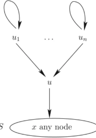
Remark 4.1. We need to use some special networks. 1. Consider Fig.9, which we shall callUn.n= 1,2,3, . . ..

The Eq_invequations solve for this ﬁgure as ui =1₂, i= 1, . . . , n.

u= 1

2n

Thus ifuattacks any nodex, its “impact” onxis the multiplicative value 1−₂1n. Fornvery large, the attack is almost negligible.

2. LetS, R be any network. Let ube a node not in S. If we add uto S

and let it attack all elements ofS, we can assume in view of (1) above that the Eqinv value ofuis ₂1n. Figure10depicts this scenario.

We suppress{u1, . . . , un} and just record thatu= 21n.

u

u1 un

Figure 9. _{Multiple attacks by undecided nodes}

S

u1 . . . un

u

xany node

(25)

Construction 4.2. Let S, R be given and let λ be a legitimate Caminada labelling giving rise to a non-preferred extension.

Let u ∈ S be a new point and assume in view of Remark 4.1 that the value ofuis very very small. Let

S=S∪ {u}

and let

R=R∪ {(u, v)|λ(v) =und}.

Let λ =λ∪ {(u,und)}.

Let Att(x)be the set of all attackers ofxin S, Rand let Att(x)be the set of all attackers ofxinS, R.

We have ifλ(x)∈ {in,out}, thenu∈ Att(x). Ifλ(x) =und, then y∈ Att(u).

Consider the following set of equations on S, R.

x= 1, ifλ(x) =in (EQ1)

x= 0, if λ(x) =out (EQ0)

x= Π(1−y)_y_∈_Att₍_x₎_in_S_{, R}, if λ(x) =und (EQU) This set of equations has a solutionf.

We claim the following 1. λ(f)is a complete extension 2. λ(f) =λ

It is clear that λ(f)(x) = λ(x), for λ(x) ∈ {in,out}. Does λ(f) agree withλ on undecided points of λ? The answer is that it must be so, becauseλ

is a preferred extension. Soλ(f)cannot be an extension with more zeros and ones thanλ.

Remark 4.3. The perceptive reader might ask why do we use those particular equations in Construction4.2(page 24)? The answer can be seen from Fig.11.

Considerλ(a) =in,λ(b) =out,λ(c) =λ(d) =und. We create Fig.12.

We take the equation

a= 1, b= 0

c= (1−d)(1−u)

d= (1−c)(1−u)

(26)

d

a b

c

Figure 11. _{A network with two cycles}

u

a b

c d

Figure 12. _{A self-attacking node attacking one of the cycles} in the network of Fig.11

The solution for the equations forc, danduare

u= 1 2

c=d=1 3

We have to insist ona= 1, b= 0. If we do not insist and write the usual equations

a= 1−b b= 1−a,

we might get a diﬀerent solution, e.g.

(27)

This not the originalλ.

Remark 4.4. This remark motivates and proves the next Theorem 4.5. We need some notation. LetQbe a set of atoms. By the models of Q(based on

Q) we mean all conjunction normal forms of atoms fromQor their negations. So, for example, ifQ={a, b, c}, we get 8 models, namely

m1=a∧b∧c .. . m8=¬a∧ ¬b∧ ¬c. If we have atoms Q1={ai}, Q2={bj}, Q3={ck}

whereQi are pairwise disjoint we can write the models ofQ1∪Q2∪Q3in the

form

α∧β∧γ

whereαis a model ofQ1, β ofQ2andγ ofQ3.

For example

α1∧β1∧γ1= (a1∧a2∧ · · ·)∧(¬b1∧b2∧ · · ·)∧(c2∧ · · ·).

Now letS, R and λ be as in Construction 4.2. Remember we assume that the value ofuis very very small, and so the attack value (1−u) is very close to 1. Considerλ and f and λ(f) again as in Construction 4.2. f is a solution of Eq_inv Eqs. (EQ1), (EQ0) and (EQU). Therefore any model ofS, say α=±s1∧ ±s2∧ ±. . .∧ ±sk∧ ±u where S ={s1, . . . , sk} will have its

probability semantics as

Pf(α= Πk_i₌₁f(±sk)))×f(±u) (*) where

f(+s) =f(s)

f(−s) = 1−f(s).

In particular, we have the following: 1. LetE+ ₌_{_e+

1, . . .} be the subset of S such thatλ(e+i ) =in. Let E− = {e−_j} be the subset ofS such thatλ(e_j−) =out. LetEund={bk}be the

set of all nodes inS such thatλ(bk) =und.

We therefore have that any modelδofS has the form

δ=_i±e+_i ∧_i±e−_j ∧_k±bk∧ ±u =α∧β±u

whereαis a model ofE+∪E− andβ is a model ofEund.

Letα1,0be the particular conjunction

α1,0= i e+_i ∧ j ¬e−_j.

(28)

Letβ be any model ofEund. ConsiderPf(δ), δ=α∧β∧ ±u. Then

by (*) we have that

Pf(δ) = 0, ifα=α1,0. (**)

SincePf is a probability, we have for anys∈S

Pf(s) =Pf

y∈Att₍_s₎¬y

.

Note that for s ∈S, s =usuch that λ(s)∈ {in,out}, u does not attacks, and so we have

Pf(s) =P(f)_y_∈_Att₍_s₎¬y

= Π_y_∈_Att₍_s₎(1−f(y)) (1) Foruwe have thatuis very small and so Pf(u) =₂1n.

Fors∈S such thatλ(s) =und, we have thatuattackssand so

Pf(s) =Pf_y_∈_Att₍_s₎¬y =Π_y_∈_Att₍_s₎(1−f(y)×1−₂1n (2) The (1− 1 2n) is the attack ofu.

We ask what are the attackers of s ∈ Eund? They cannot be nodes x

such thatλ(x) = in, because then swould be out. So the value of f(y), (for

y∈Att(s)) is either 0 or a value in (0,1). So we can continue and write

Pf(s) = 1− 1 2n Π_y_∈_Att₍_s₎ λ(y) =und (1−f(y)) (3) Note that 0< Pf(s)< 1, because all the f(y), for λ(y) = und, satisfy 0< f(y)<1.

We also have

all modelsm

Pf(m) = 1. (4)

Since (**) holds, we need consider only modelsmof the formα1,0∧β∧±u.

We can write

1 = β∧±u

Pf(α1,0∧β∧ ±u) (5)

whereβ is a model ofEund. Let us analyse (5) a bit more.

Assumeβ =_k±bk. So

Pf(α0,1∧β∧u) +Pf(α0,1∧β∧ ¬u) = Πkf(±bk). (6) We thus get that:

β

(29)

(7) says something very interesting. It says that f restricted to Eund

gives a proper probability distribution on the models ofEund.

This combined with (3) gives us the following result.

Consider (Eund, Rund) whereRund=REund. Thenf Eundis a proper

probability distribution on (Eund, Rund).

Does it satisfy the proper equations? Lets∈Eund. Do we have

Pund(s)=? Pund _y_∈_E und yRx ¬y Let us check.

The real equation is

Pund(s) =Pund _y_∈_E und [1ex]yRx ¬y ×(1−u) (8) Sinceuis very small, we have a very good approximation.5

We can now deﬁne a probabilityP onS, R. Letm=α∧β be a model, whereαis a model forE+_∪_E− _and_β _{is a model for}_E

und.

Then deﬁneP as follows

P(α∧β) = 0, ifα=¬α1,0

P(α∧β) =Pund(β), ifα=α1,0

We need to show that approximately

P(s) =P

y∈Att(s)¬y

Ifs∈E+∪E− this follows from ( 1). Ifs∈Eund, this follows from ( 3) and ( 8).

Note that since thef involved came from Eqinvequations,P satisﬁes the

following onS, R.

P(s) = 0, if somey∈Att(s)P(y) = 1

P(s) = 1, if for ally∈Att(s), P(y) = 0

P(s) = undecided, otherwise.

(9)

5_{The perceptive reader might ask what happens if we let} _u_{converge to 0? The answer is}

that we get a proper Eq_inv extension. However, this may be an all undecided extension (which is what we do want), or it may be a complete extension properly containing all the undecided extensions (which is not what we want!).

We may decide to do what physicists do to their equations. Write the equations in full and simply neglect any item containing higher orderu, i.e.,u2, u3, etc. This is reasonable when the value of each node is small.

(30)

Theorem 4.5.

1. Let S, R be a network and letλ be a legitimate Caminada labelling on

S. Then there exists a Method 1 probability distributionPλ, which almost satisfies Eq.(E3), namely for everyε, there exists a Method 1 probability

Pλ depending on ε, such that for every x and its attackers yi, we have |Pλ(x)−Pλ(∧¬yi)|< ε, such that

λ(x) =in, if Pλ(x) = 1

λ(x) =out, if Pλ(x) = 0

λ(x) =und, if0< Pλ(x)<1. 2. P is obtained as follows

Case 1.λis a preferred extension. Then letf be a solution of Eq_inv forS, R. LetPλ=f.

Case 2.λis not a preferred extension.

Let E_undλ ={x|λ(x) = und}. ConsiderS, R, where S =Eλ_und∪

{u}, whereuis a new point not inS with value almost 0.

R=REundλ ∪ {u} ×Eundλ .

Then S, R has only one extension (all undecided). Let f be a solution to Eq_inv on S, R. We now definePλ onS, R.

Let α1,0=

λ(x)=inx∧

λ(y)= out¬y.

Let m =α∧β be an arbitrary model of S, where αis a model of {x|λ(x)∈ {in,out}andβ is a model ofE_undλ . DefinePλ(α∧β)to be

Pλ(α∧β= 0 ifα=α1,0

Pλ(α1,0∧β) =f(β)

whereβ =_s_∈_Eλ und±s andf(β) = Π_±_s_in_βf(±s).

Proof. Follows from the considerations of Remark4.4. Example 4.6. Let us show how Theorem4.5works by doing a few examples.

1. Consider the network of Fig. 11 and the extension λ mentioned there, namelyλ(a) =in,λ(b) =out,λ(c) =λ(d) =und.

Following our algorithms we look at the{c, d, u}part of Fig.12and solve the equations. We getu=1

2, c=d=13.

The probabilityPλwill be as follows:

Pλ(α∧β) = 0 ifα=a∧ ¬b. Now look at Pλ(a∧ ¬b∧c∧d) =13×13 = 19 Pλ(a∧ ¬b∧c∧ ¬d) =1₃×2₃ = 2₉ Pλ(a∧ ¬b∧ ¬c∧d) =23×13 = 29 Pλ(a∧ ¬b∧ ¬c∧ ¬d) =23×23 =49.

(31)

2. Let us look at Fig.13.

Withλ(a) =in,λ(b) =out, λ(c) =λ(d) =und.

The{c, d}part is Fig.2. Here we solve the equations on the{c, d, u}

part associated with {c, d}, which is the same as Fig. 3. The solution is found in Example2.5, withu= 1₂.

We getu= 1

2;c= 0.36,1−c= 0.764, d= 0.382,1−d= 0.618. The

probabilityPλ of this case isPλ(α∧β) = 0, ifα=a∧ ¬b.

Pλ(a∧ ¬b∧c∧d) = 0.236×0.382 = 0.09 Pλ(a∧ ¬b∧c∧ ¬d) = 0.236×0618 = 0.146 Pλ(a∧ ¬b∧ ¬c∧d) = 0.764×0.382 = 0.292 Pλ(a∧ ¬b∧ ¬c∧ ¬d) = 0.764×0.618 = 0.472. Indeed 0.09 + 0.146 + 0.292 + 0.472 = 1.000.

We now discuss imposing probability on instantiated networks such as ASPIC+. We begin with simple instantiations into classical propositional logic.

Definition 4.7. 1. An abstract instantiated network (into classical propo-sitional logic) has the form A = S, R, I, where S, R is an abstract argumentation network andIis a mapping associating with each x∈S, a well-formed formulaI(x) =ϕx of classical propositional logic.

2. For anyAas in4.7, we associate the theory Δ_A={ϕx↔ ∧(y,x)∈R¬ϕy|x ∈S}.

3. A semantic probability modelP onAis a probability distribution on the models based onS such that for allx∈S, we have:

P(ϕx) =P(∧(y,x)∈R¬ϕy)

Example 4.8. Consider Fig. 14 where part (b) is an instatiation of part (a) withI(x) =a1∨a2andI(a3) =a3. The equations any probability assignment

d

a b

c

Figure 13. _{Augmented network of Fig.} ₂ _{with node} _a_as _c andbasdand an extra cycle

(32)

a1∨a2 a3 (b) x a3 (a)

Figure 14. _a_{A network and}_b_{one of its instantiations with}

x=a1∨a2

0.236 a b0.382

Figure 15. _{The Eq}_inv _{solution to the networks of Figs.}₂_and₃

needs to satisfy are

P(a1∨a2) = 1

P(a3) =P(¬(a1∨a2))

=P(¬a1∧ ¬a2)

= 0.

If we letP(a1) = x, P(a2) = 1−x, P(a3) = 0, with x∈ [0,1], thenP

satisﬁes the equations. Compare with Example3.4.

5. Comparison with the Literature

There are several probabilistic argumentation papers around. This is a hot topic in 2014. We highlight two main points of view. The external and the internal views.

LetS, Rbe a network and let fbe a function from S to [0,1]. We can regardfas giving a probability number to eachx∈S. The internal probability is where the above numbers signify the value of the argument. Its truth, its reliability, its probability of being eﬀective, etc., or whatever measure we attach to it as an argument. Figure15represents in this case the Eqinv solution (and

hence probability) of the network of Figs.2and3. The external view is to think of f(x) as the probability of the predicate “x∈ S”. That is, the probability that the argumentxis present in S. Consider again Fig.15.

The probability thatais in the network is 0.236 and the probability thatb

(33)

both{a, b}is 0.236×0.388 = 0.09. The probability that the network contains onlyais 0.236×(1−0.382) = 0.1458. The probability that the network contains onlyb is 0.382×(1−0.236) = 0.292 and the probability that the network is empty is (1−0.236)×(1−0.382) = 0.472. It is clear why we are calling this view an external probability view. It imposes probability externally expressing uncertainty on what the network graph is. This is done either by giving the probability to points or more generally by giving probability directly to subsets

GofS, expressing the probability that the graph is really that subset ofSwith

Rrestricted to G. This external view has value in dialogue argumentation or negotiation when we try to estimate what network our opponent is reasoning with. The problem with this external view is how to connect with the attack relation. Note that mathematically in the external view we have probabilities on points inS or probabilities on subsets of S, which are the same options as in our internal view, but the understanding of them is diﬀerent. We in the internal view considered the subset as a classical model, while the external view considers it as a subnetwork. When we use the internal view, we can connect it with the attack relation via the equational approach [Eq. (E3)], but how would the external view connect with the attack relation? We can ask, for example, how to get a value for a single point to be “in” an extension? Intuitively, looking back at Fig.15, we can say the point a for example is “in” in case the network is

{a}and is also “in” in one of the three extensions in case the network is{a, b}. So we might take the “in” value to be 0.1458+0.09/3 = 0.1458+0.03 = 0.1758. The connection with the attack relation can be done perhaps through the probabilities for admissible sets, since being admissible is connected with the attack relation. There are problems, however, with this approach.

Hunter [7] was trying to lay some foundations for this view, following the papers [3,9]. See also a good summary in Hunter [8]. Hunter was trying to ﬁnd a connection between the external probability view and some reasonable values we can give to admissible subsets. He proposes restrictions on the probability function onS. We are not going to discuss or reproduce Hunter’s arguments here. It suﬃces to say that possibly a subsequent paper of ours will critically examine the external view and compare with the internal view.

Let us now compare our work with that of Thimm, [13], whose approach is also internal. We quote from [13]:

In this paper we use another interpretation for probability, that ofsubjective probability [11]. There, a probability P(X) for someX ∈ X denotes thedegree of belief we put into X. Then a probability function P can be seen as an epistemic state of some agent that has uncertain beliefs with respect to X. In probabilistic reasoning [11,12], this interpretation of probability is widely used to model uncertain knowledge representation and reasoning.

In the following, we consider probability functions on sets of arguments of an abstract argumentation frameworks. Let AF = (Arg,→) be some ﬁxed abstract argumentation