University of Zurich
Zurich Open Repository and Archive
Winterthurerstr. 190 CH-8057 Zurich http://www.zora.uzh.ch
Year: 2008
Control of the false discovery rate under dependence using the
bootstrap and subsampling
Romano, J P; Shaikh, A M; Wolf, M
Romano, J P; Shaikh, A M; Wolf, M (2008). Control of the false discovery rate under dependence using the bootstrap and subsampling. Test, 17(3):417-442.
Postprint available at: http://www.zora.uzh.ch
Posted at the Zurich Open Repository and Archive, University of Zurich. http://www.zora.uzh.ch
Originally published at: Test 2008, 17(3):417-442.
Romano, J P; Shaikh, A M; Wolf, M (2008). Control of the false discovery rate under dependence using the bootstrap and subsampling. Test, 17(3):417-442.
Postprint available at: http://www.zora.uzh.ch
Posted at the Zurich Open Repository and Archive, University of Zurich. http://www.zora.uzh.ch
Control of the false discovery rate under dependence using the
bootstrap and subsampling
Abstract
This paper considers the problem of testing s null hypotheses simultaneously while controlling the false discovery rate (FDR). Benjamini and Hochberg (1995) provide a method for controlling the FDR based on p-values for each of the null hypotheses under the assumption that the p-values are independent. Subsequent research has since shown that this procedure is valid under weaker assumptions on the joint distribution of the p-values. Related procedures that are valid under no assumptions on the joint distribution of the p-values have also been developed. None of these procedures, however, incorporate information about the dependence structure of the test statistics. This paper develops methods for control of the FDR under weak assumptions that incorporate such information and, by doing so, are better able to detect false null hypotheses. We illustrate this property via a simulation study and two empirical applications. In particular, the bootstrap method is competitive with methods that require independence if independence holds, but it outperforms these methods under dependence.
Control of the False Discovery Rate under Dependence using the
Bootstrap and Subsampling
Joseph P. Romano
Departments of Econmics and Statistics Stanford University [email protected] Azeem M. Shaikh Department of Economics University of Chicago [email protected] Michael Wolf∗
Institute for Empirical Research in Economics University of Zurich
[email protected] October 2008
Abstract
This paper considers the problem of testingsnull hypotheses simultaneously while con-trolling thefalse discovery rate(FDR). Benjamini and Hochberg (1995) provide a method for controlling the FDR based on p-values for each of the null hypotheses under the as-sumption that the p-values are independent. Subsequent research has since shown that this procedure is valid under weaker assumptions on the joint distribution of thep-values. Related procedures that are valid under no assumptions on the joint distribution of the
p-values have also been developed. None of these procedures, however, incorporate infor-mation about the dependence structure of the test statistics. This paper develops methods for control of the FDR under weak assumptions that incorporate such information and, by doing so, are better able to detect false null hypotheses. We illustrate this property via a simulation study and two empirical applications. In particular, the bootstrap method is competitive with methods that require independence if independence holds, but it outper-forms these methods under dependence.
∗Corresponding Author. Address for correspondence: Michael Wolf, Institute for Empirical Research in Economics, University of Zurich, Bluemlisalpstrasse 10, CH-8006 Zurich, Switzerland, Email: [email protected], Phone: +41-44 634 5096, Fax: +41-44 634 4907.
KEY WORDS: Bootstrap, Subsampling, False Discovery Rate, Multiple Testing, Stepdown Procedure.
MSC Codes: 62G09, 62G10, 62G20, 62H15.
ACKNOWLEDGMENTS: We are grateful to Harry Joe for providing Rroutines to generate random correlation matrices. The research of the first author has been supported by the National Science Foundation grant DMS-0707085. The research of the third author has been supported by the University Research Priority Program “Finance and Financial Markets”, University of Zurich, and by the Spanish Ministry of Science and Technology and FEDER, grant MTM2006-05650.
1
Introduction
Consider the problem of testing s null hypotheses simultaneously. A classical approach to dealing with the multiplicity problem is to restrict attention to procedures that control the probability of one or more false rejections, which is called the familywise error rate(FWER). When s is large, however, the ability of such procedures to detect false null hypotheses is limited. For this reason it is often preferred in such situations to relax control of the FWER in exchange for improved ability to detect false null hypotheses.
To this end, several ways of relaxing the FWER have been proposed. Hommel and Hoffman (1988) and Lehmann and Romano (2005a) consider control of the probability of k or more false rejections for some integer k ≥1, which is termed the k-FWER. Obviously, controlling the 1-FWER is the same as controlling the usual FWER. Lehmann and Romano (2005a) also consider control of thefalse discovery proportion(FDP), defined to be the fraction of rejections that are false rejections (with the fraction understood to be 0 in the case of no rejections). Given a user-specified value of γ, control of the FDP means control of the probability that the FDP is greater than γ. Note that when γ = 0 control of the FDP reduces to control of the usual FWER. Methods for control of thek-FWER and the FDP based onp-values for each null hypothesis are discussed in Lehmann and Romano (2005a), Romano and Shaikh (2006a), and Romano and Shaikh (2006b). These methods are valid under weak or no assumptions on the dependence structure of thep-values, but they do not attempt to incorporate information about the dependence structure of the test statistics. Methods that incorporate such information and
are thus better able to detect false null hypotheses are described in van der Laan et al. (2004), Romano and Wolf (2007), and Romano et al. (2008).
A popular third alternative to control of the FWER is control of the false discovery rate
(FDR), defined to be the expected value of the FDP. Control of the FDR has been suggested in a wide area of applications, such as educational evaluation (Williams et al., 1999), clinical trials (Mehrotra and Heyse, 2004), analysis of microarray data (Drigalenko and Elston, 1997; and Reiner et al., 2003), model selection (Abramovich and Benjamini, 1996; and Abramovich et al., 2006), and plant breeding (Basford and Tukey, 1997). Benjamini and Hochberg (1995) provide a method for controlling the FDR based onp-values for each null hypothesis under the assumption that the p-values are independent. Subsequent research has since shown that this procedure remains valid under weaker assumptions on the joint distribution of the p-values. Related procedures that are valid under no assumptions on the joint distribution of thep-values have also been developed; see Benjamini and Yekutieli (2001). Yet procedures for control of the FDR under weak assumptions that incorporate information about the dependence structure of the test statistics remain unavailable. This paper seeks to develop methods for control of the FDR that incorporate such information and, by doing so, are better able to detect false null hypotheses.
The remainder of the paper is organized as follows. In Section 2 we describe our notation and setup. Section 3 summarizes previous research on methods for control of the FDR. In Sec-tion 4 we provide some motivaSec-tion for our methods for control of the FDR. A bootstrap-based method is then developed in Section 5. The asymptotic validity of this approach relies upon an exchangeability assumption, but in Section 6 we develop a subsampling-based approach whose asymptotic validity does not depend on such an assumption. Section 7 sheds some light on the finite-sample performance of our methods and some previous proposals via simulations. We also provide two empirical applications in Section 8 to further compare the various methods. Section 9 concludes.
2
Setup and Notation
A formal description of our setup is as follows. Suppose data X = (X1, . . . , Xn) is available
from some probability distributionP ∈Ω. Note that we make no rigid requirements for Ω; it may be a parametric, semiparametric or a nonparametric model. A general hypothesisH may be viewed as a subset ω of Ω. In this paper we consider the problem of simultaneously testing null hypotheses Hi : P ∈ ωi, i = 1, . . . , s on the basis of X. The alternative hypotheses are
understood to beH′
i :P 6∈ωi, i= 1, . . . , s.
We assume that test statistics Tn,i, i = 1, . . . , s are available for testing Hi, i = 1, . . . , s.
Large values of Tn,i are understood to indicate evidence against Hi. Note that we may take Tn,i=−pˆn,i, where ˆpn,i is a p-value for Hi. Ap-value for Hi may be exact, in which case ˆpn,i
satisfies
P{pˆn,i≤u} ≤u for anyu∈(0,1) andP ∈ωi (1)
or asymptotic, in which case lim sup
n→∞ P{pˆn,i≤u} ≤u for anyu∈(0,1) andP ∈ωi . (2)
In this article, we consider stepdownmultiple testing procedures. Let
Tn,(1) ≤ · · · ≤Tn,(s)
denote the ordered test statistics (from smallest to largest) and let
H(1), . . . , H(s)
denote the corresponding null hypotheses. Stepdown multiple testing procedures first compare the most significant test statistic, Tn,(s), with a suitable critical valuecs. IfTn,(s) < cs, then
the procedure rejects no null hypotheses; otherwise, the procedure rejects H(s) and then ‘steps
down’ to the second most significant null hypothesis H(s−1). If Tn,(s−1) < cs−1, then the
procedure rejects no further null hypotheses; otherwise, the procedure rejectsH(s−1) and then ‘steps down’ to the third most significant null hypothesis H(s−2). The procedure continues in this fashion until either one rejects H(1) or one does not reject the null hypothesis under consideration. More succinctly, a stepdown multiple testing procedure rejects
H(s), . . . , H(s−j∗) ,
where j∗ is the largest integer j that satisfies
Tn,(s)≥cs, . . . , Tn,(s−j)≥cs−j ;
if no such j exits, the procedure does not reject any null hypotheses.
We will construct stepdown multiple testing procedures that control the false discovery rate (FDR), which is defined to be the expected value of thefalse discovery proportion (FDP). Denote by I(P) the set of indices corresponding to true null hypotheses; that is,
For a given multiple testing procedure, let F denote the number of false rejections and letR
denote the total number of rejections; that is,
F = |{1≤i≤s:Hi rejected andi∈I(P)}| R = |{1≤i≤s:Hi rejected}|.
Then, the false discovery proportion (FDP) is defined as follows: FDP = F
max{R,1} .
Using this notation, the FDR is simplyE[FDP]. A multiple testing procedure is said to control the FDR at level α if
FDRP =EP[FDP]≤α for allP ∈Ω.
A multiple testing procedure is said to control the FDR asymptotically at level α if lim sup
n→∞ FDRP ≤α for all P ∈Ω. (4)
We will say that a procedure is asymptotically valid if it satisfies (4). Methods that control the FDR can typically only be derived in special circumstances. In this paper, we will instead pursue procedures that are asymptotically valid under weak assumptions.
3
Previous Methods for Control of the FDR
In this section, we summarize the existing literature on methods for control of the FDR. The first known method proposed for control of the FDR is the stepwise procedure of Benjamini and Hochberg (1995) based on p-values for each null hypothesis. Let
ˆ
pn,(1) ≤ · · · ≤pˆn,(s) denote the ordered values of the p-values and let
H(1), . . . , H(s)
denote the corresponding null hypotheses. Note that in this case the null hypotheses are ordered from most significant to least significant, since small values of ˆpn,iare taken to indicate evidence
against Hi. For 1≤j≤s, let
αj = j
sα . (5)
Then, the method of Benjamini and Hochberg (1995) rejects null hypotheses H(1), . . . , H(j∗),
where j∗ is the largestj such that
ˆ
Of course, if no such j exists, then the procedure rejects no null hypotheses.
Benjamini and Hochberg (1995) prove that their method controls the FDR at level α
if the p-values satisfy (1) and are independent. Benjamini and Yekutieli (2001) show that independence can be replaced by a weaker condition known as positive regression dependency; see their paper for the exact definition. It can also be shown that the method of Benjamini and Hochberg (1995) provides asymptotic control of the FDR at level α if thep-values satisfy (2) instead of (1) and this weaker dependence condition holds.
On the other hand, the method of Benjamini and Hochberg (1995) fails to control the FDR at levelαwhen thep-values only satisfy (1). Benjamini and Yekutieli (2001) show that control of the FDR can be achieved under only (1) if αj defined in (5) are replaced by
αj = j s α Cs ,
where Ck =Pkr=1r1. Note thatCs ≈log(s) + 0.5, so this method can have much less power
than the method of Benjamini and Hochberg (1995). For example, when s = 1,000, then
Cs = 7.49. As before, it can be shown that this procedure provides asymptotic control of the FDR at level α if the p-values satisfy (2) instead of (1).
Even when sufficient conditions for the method of Benjamini and Hochberg (1995) to control the FDR hold, it is conservative in the following sense. It can be shown that
FDRP ≤ s0
sα ,
where s0 = |I(P)|. So, unless s0 = s, the power of the procedure could be improved by
replacing the αj defined in (5) by
αj = j s0
α .
Of course, s0 is unknown in practice, but there exist several approaches in the literature to
estimate s0. For example, Storey et al. (2004) suggest the following estimator:
ˆ
s0 =
#{pˆn,j > λ}+ 1
1−λ , (6)
where λ ∈ (0,1) is a user-specified parameter. The reasoning behind this estimator is the following. As long as each test has reasonable power, then most of the “large”p-values should correspond to true null hypotheses. Therefore, one would expect abouts0(1−λ) of thep-values
to lie in the interval (λ,1], assuming that thep-values corresponding to the true null hypotheses have approximately a uniform [0,1] distribution. Adding one in the numerator of (6) is a small-sample adjustment to make the procedure slightly more conservative and to avoid an estimator
of zero fors0. Having estimateds0, one then applies the procedure of Benjamini and Hochberg
(1995) with the αj defined in (5) replaced by
ˆ
αj = j ˆ
s0
α .
Storey et al. (2004) prove that this adaptive procedure controls the FDR asymptotically when-ever the p-values satisfy (2) and a weak dependence condition holds. This condition includes independence, dependence within blocks, and mixing-type situations, but, unlike Benjamini and Yekutieli (2001), it does not allow for arbitrary dependence among the p-values. It ex-cludes, for example, the case in which there is a constant correlation across allp-values. Related work is found in Genovese and Wasserman (2004) and Benjamini and Hochberg (2000).
The adaptive procedure of Storey et al. (2004) can be quite liberal under positive depen-dence, such as in a scenario with constant positive correlation. For this reason, Benjamini et al. (2006) develop an alternative procedure, which works as follows:
Algorithm 3.1 (BKY Algorithm)
1. Apply the procedure of Benjamini and Hochberg (1995) at nominal levelα∗ =α/(1 +α). Let r be the number of rejected hypotheses. If r = 0, then do not reject any hypothesis and stop; ifr =s, then reject all shypotheses and stop; otherwise continue.
2. Apply the procedure of Benjamini and Hochberg (1995) with the αj defined in (5) re-placed by ˆαj = ˆsj0α
∗, where ˆs
0 =s−r.
Benjamini et al. (2006) prove that this procedure controls the FDR whenever the p-values satisfy (2) and are independent of each other. They also provide simulations which suggest that this procedure continues to control the FDR under positive dependence.
Benjamini and Liu (1999) provide a stepdown method for control of the FDR based on
p-values for each null hypothesis that satisfy (1) and are independent. Sarkar (2002) extends the results of Benjamini and Hochberg (1995), Benjamini and Liu (1999), and Benjamini and Yekutieli (2001) to generalized stepup-stepdown procedures, yet the methods he considers, like those described above, do not incorporate the information about the dependence structure of the test statistics. In the following sections, we develop multiple testing procedures for asymptotic control of the FDR under weak assumptions that incorporate such information, and, by doing so, are better able to detect false hypotheses. Our procedures build upon the work of Troendle (2000), who suggests a procedure for asymptotic control of the FDR that
incorporates information about the dependence structure of the test statistics, but relies upon the restrictive parametric assumption that the joint distribution of the test statistics is given by a symmetric multivariatet-distribution. Yekutieli and Benjamini (1999) also provide a method for asymptotic control of the FDR that exploits information about the dependence structure of the test statistics to improve the ability to detect false null hypotheses, but their analysis requires subset pivotality and that the test statistics corresponding to true null hypotheses are independent of those corresponding to false null hypotheses. Although our analysis will require neither of these restrictive assumptions, the asymptotic validity of our bootstrap approach will rely upon an exchangeability assumption. The subsampling approach we will develop subsequently, however, will not even require this restriction.
4
Motivation for Methods
In order to motivate our procedures, first note that for any stepdown procedure based on critical values c1, . . . cs we have that
FDRP = EP[ F max{R,1}] = X 1≤r≤s 1 rEP[F|R =r]P{R=r} = X 1≤r≤s 1 rE[F|R=r]P{Tn,(s) ≥cs, . . . , Tn,(s−r+1)≥cs−r+1, Tn,(s−r)< cs−r} ,
where the event Tn,s−r < cs−r is understood to be vacuously true when r = s. As before,
let s0 = |I(P)| and assume without loss of generality that I(P) = {1, . . . , s0}. Under weak
assumptions, we will show that all false hypotheses will be rejected with probability tending to one. For the time being, assume that this is the case. Let Tn,r:t denote the rth largest of
the ttest statistics Tn,1, . . . , Tn,t; in particular, when t=s0,Tn,r:s0 denotes the rth largest of
the test statistics corresponding to the true hypotheses. Then, with probability approaching one, we have that
FDRP = X s−s0+1≤r≤s r−s+s0 r P{Tn,s0:s0 ≥cs0, . . . , Tn,s−r+1:s0 ≥cs−r+1, Tn,s−r:s0 < cs−r}, (7) where the event Tn,s−r:s0 < cs−r is again understood to be vacuously true whenr=s.
Our goal is to ensure that (7) is bounded above by α for any P, at least asymptotically. To this end, first consider any P such thats0=|I(P)|= 1. Then, (7) is simply
FDRP =
1
A suitable choice ofc1 is thus the smallest value for which (8) is bounded above byα; that is,
c1= inf{x∈R:
1
sP{Tn,1:1 ≥x} ≤α}.
Note that ifsα≥1, then c1 so defined is equal to −∞.
Having determinedc1, now consider any P such that s0= 2. Then, (7) is simply
1
s−1P{Tn,2:2≥c2, Tn,1:2< c1}+ 2
sP{Tn,2:2≥c2, Tn,1:2≥c1}. (9)
A suitable choice ofc2 is therefore the smallest value for which (9) is bounded above byα.
In general, having determined c1, . . . , cj−1, the jth critical value may be determined by
considering P such that s0 =j. In this case, (7) is simply
FDRP =
X
s−j+1≤r≤s
r−s+j
r P{Tn,j:j ≥cj, . . . , Tn,s−r+1:j ≥cs−r+1, Tn,s−r:j < cs−r}. (10)
An appropriate choice of cj is thus the smallest value for which (10) is bounded above by α.
Note that when j=s, (10) simplifies to
P{Tn,s:s≥cs},
so equivalently
cs= inf{x∈R:P{Tn,s:s≥x} ≤α} .
Of course, the above choice of critical values is infeasible since it depends on the unknownP
through the distribution of the test statistics. We therefore focus on feasible constructions of the critical values based on the bootstrap and subsampling.
5
A Bootstrap Approach
In this section, we specialize our framework to the case in which interest focuses on a parameter vector
θ(P) = (θ1(P), . . . , θs(P)).
The null hypotheses may be one-sided, in which case
Hj :θj ≤θ0,j vs. Hj′ :θj > θ0,j (11)
or the null hypotheses may be two-sided, in which case
In the next section, however, we will return to more general null hypotheses. Test statistics will be based on an estimate ˆθn= (ˆθn,1, . . . ,θˆn,s) of θ(P) computed using the dataX. We will
consider ‘studentized’ test statistics
Tn,j =√n(ˆθn,j−θ0,j)/σˆn,j (13)
for the one-sided case (11) or
Tn,j =√n|θˆn,j−θ0,j|/σˆn,j (14)
for the two-sided case (12). Note that ˆσn,j may either be identically equal to 1 or an estimate
of the standard deviation of √n(ˆθn,j −θ0,j). This is done to keep the notation compact; the
latter is preferable from our point of view but may not always be available in practice. Recall that the construction of critical values in the preceding section was infeasible because of its dependence on the unknown P. For the bootstrap construction, we therefore simply replace the unknown P with a suitable estimate ˆPn. To this end, let X∗ = (X1∗, . . . , Xn∗) be
distributed according to ˆPnand denote byTn,j∗ , j= 1, . . . , s test statistics computed from X∗.
For example, if Tn,j is defined by (13) or (14), then
Tn,j∗ =√n(ˆθ∗n,j−θj( ˆPn))/σˆn,j∗ (15)
or
Tn,j∗ =√n|θˆ∗n,j−θj( ˆPn)|/σˆn,j∗ , (16) respectively, where ˆθ∗
n,j is an estimate of θj computed from X∗ and ˆσ∗n,j is either identically
equal to 1 or an estimate of the standard deviation of √n(ˆθn,j∗ −θj( ˆPn)) computed from X∗.
For the validity of this approach, we require that the distribution of T∗
n,j provides a good
approximation to the distribution of Tn,j whenever the corresponding null hypothesis Hj is
true, but, unlike Westfall and Young (1993), we do not require subset pivotality. The exact choice of ˆPn will, of course, depend on the nature of the data. If the data X = (X1, . . . , Xn)
are i.i.d., then a suitable choice of ˆPn is the empirical distribution, as in Efron (1979). If, on
the other hand, the data constitute a time series, then ˆPn should be estimated using a suitable
time series bootstrap method; see Lahiri (2003) for details.
Given a choice of ˆPn, define the critical values recursively as follows: having determined
ˆ
cn,1, . . . ,ˆcn,j−1, compute ˆcn,j according to the rule
ˆ cn,j = inf{c∈R: X s−j+1≤r≤s r−s+j r Pˆn{T ∗ n,j:j ≥c, . . . , Tn,s∗ −r+1:j ≥cn,sˆ −r+1, Tn,s∗ −r:j <cn,sˆ −r} ≤α}. (17)
Remark 5.1 It is important to be clear about the meaning of the notationT∗
n,r:t, withr≤t,
in (17). By analogy to the “real” world, it should denote the rth smallest of the observations corresponding to the first t true null hypotheses. However, the ordering of the true null hypotheses in the bootstrap world is not 1,2, . . . , s, but it is instead determined by the ordering
H(1), . . . , H(s) from the real world. So if the permutation {k1, . . . , ks} of {1, . . . , s} is defined
such that Hk1 = H(1), . . . , Hks = H(s), then T ∗
n,r:t is the rth smallest of the observations Tn,k∗ 1, . . . , Tn,k∗ t.
Remark 5.2 Note that typically it will not be possible to compute closed form expressions for the probabilities under ˆPn required in (17). In such cases, the required probabilities may instead be computed using simulation to any desired degree of accuracy.
We now provide conditions under which the stepdown procedure with critical values defined by (17) satisfies (4). The following result applies to the case of two-sided null hypotheses, but the one-sided case can be handled using a similar argument. In order to state the result, we will require some further notation. ForK ⊆ {1, . . . , s}, letJn,K(P) denote the joint distribution of
(√n(ˆθn,j −θj(P))/σˆn,j :j∈K) .
It will also be useful to define the quantile function corresponding to a c.d.f. G(·) on R as
G−1(α) = inf{x∈R:G(x)≥α}.
Theorem 5.1 Consider the problem of testing the null hypotheses Hi, i = 1, . . . , s given
by (12) using test statistics Tn,i, i = 1, . . . , s defined by (14). Suppose that Jn,{1,...,s}(P)
con-verges weakly to a limit law J{1,...,s}(P), so that Jn,I(P)(P) converges weakly to a limit law
JI(P)(P). Suppose further that JI(P)(P)
(i) has continuous one-dimensinal marginal distributions;
(ii) has connected support, which is denoted by supp(JI(P)(P));
(iii) is exchangeable. Also, assume
ˆ
σn,j →P σj(P) ,
where σj(P)>0 is nonrandom. Let Pˆn be an estimate ofP such that
where ρ is any metric metrizing weak convergence in Rs.
Then, for the stepdown method with critical values defined by (17)
lim sup
n→∞
FDRP ≤α .
We will make use of the following lemma in our proof of the preceding theorem:
Lemma 5.1 Let X be a random vector on Rs with distribution P. Define f :Rs→R by the
rule f(x) =x(k) for some fixed 1≤k≤s, where
x(1)≤ · · · ≤x(s) .
Suppose that (i) the one-dimensional marginal distributions of P have continuous c.d.f.s and
(ii) supp(X) is connected. Then, f(X) has a continuous and strictly increasing c.d.f.
Proof: To see that the c.d.f. of f(X) is continuous, simply note that
P{f(X) =x} ≤ X
1≤i≤s
P{Xi =x}= 0,
where the final equality follows from assumption (i). To see that the c.d.f. of f(X) is strictly increasing, suppose by way of contradiction that there exists a < b such that P{f(X) ∈ (a, b)} = 0, but P{f(X) ≤ a} > 0 and P{f(X) ≥ b} > 0. Thus, there exists x ∈ supp(X) such that f(x)≤a andx′∈supp(X) such thatf(x′)≥b. Consider the set
Aa,b={x∈supp(X) :a < f(x)< b} .
By continuity of f(x) and assumption (ii), Aa,b is non-empty. Moreover, again by continuity
of f(x),Aa,b must contain an open subset of supp(X) (relative to the topology on supp(X)).
It therefore follows by the definition of supp(X) that
P{X∈Aa,b}=P{f(X)∈(a, b)}>0 ,
which yields the desired contradiction.
Remark 5.3 An important special case of Lemma 5.1 is the case in which X is distributed as a multivariate normal random vector with mean µ and covariance matrix Σ. In this case, assumptions (i) - (ii) of the lemma are implied by the very mild restriction that Σi,i >0 for
Remark 5.4 Note that even in the case in whichs= 1, sof(x) =x, both assumptions (i) and (ii) in Lemma 5.1 are necessary to conclude that the distribution of f(X) is continuous and strictly increasing. Therefore, the assumptions used in Lemma 5.1 seem as weak as possible.
Proof of Theorem 5.1Without loss of generality, suppose thatH1, . . . , Hs0 are all true and
the remainder false.
In order to illustrate better the main ideas of the proof, we first consider the case in which
P is such that the number of true hypotheses is s0 = 1. The initial step in our argument is to
show that all false null hypotheses are rejected with probability tending to 1. Sinceθj(P)6=θ0,j
forj ≥2, it follows that
Tn,j =n1/2|θn,jˆ −θ0,j|/σn,jˆ → ∞P
forj ≥2. On the other hand, for j= 1, we have that
Tn,j =OP(1).
Therefore, to show all false hypotheses are rejected with probability tending to one, it suffices to show that the critical values ˆcn,j are all uniformly bounded above in probability for j≥2.
Recall that ˆcn,j is defined as follows: having determined ˆcn,1, . . . ,ˆcn,j−1, ˆcn,j is the infimum
over all c∈Rfor which
X s−j+1≤r≤s r−s+j r Pˆn{T ∗ n,j:j ≥c, . . . , Tn,s∗ −r+1:j ≥ˆcn,s−r+1, Tn,s∗ −r:j <ˆcn,s−r} (19)
is bounded above by α. Note that (19) can be bounded above by
jPˆn{Tn,j∗ :j ≥c} ,
which can in turn be bounded above by
sPˆn{Tn,s∗ :s≥c} . (20)
It follows that the set of c∈Rfor which (20) is bounded above by α is a subset of the set of
c∈R for which (19) is bounded above byα. Therefore, ˆcn,j is bounded above by the 1−α/s
quantile of the (centered) bootstrap distribution of the maximum of all s variables. In order to describe the asymptotic behavior of this bootstrap quantity, let
Mn(x, P) =P{max
1≤j≤s{n
1/2
|θn,jˆ −θj|/ˆσn,j} ≤x} ,
and let ˆMn(x) denote the corresponding bootstrap c.d.f. given by
ˆ
Pn{max
1≤j≤s{n
1/2|θˆ∗
In this notation, the previously derived bound for ˆcn,j may be restated as ˆ cn,j ≤Mˆn−1 1− α s .
By the Continuous Mapping Theorem,Mn(·, P) converges in distribution to a limit distribution
M(·, P), and the assumptions imply this limiting distribution is continuous. Choose 0< ǫ < αs
so that M(·, P) is strictly increasing at M−1(1−αs +ǫ, P). For such anǫ, ˆ Mn−11−α s +ǫ P →M−11− α s +ǫ, P .
Therefore, ˆcn,j is with probability tending to one less thanM−1 1−αs +ǫ, P
. The claim that ˆ
cn,j is bounded above in probability is thus verified.
It now follows that, in the cases0 = 1,
FDRP =
1
sP{Tn,1≥cˆn,1}+oP(1).
The critical value ˆcn,1 is the 1−αsquantile of the distribution ofTn,∗1 under ˆPn. If 1−αs≤0,
then ˆcn,1 is defined to be−∞, in which case,
FDRP = 1
s +oP(1)≤α+oP(1) .
The desired conclusion thus holds. If, on the other hand, 1−αs >0, then we argue as follows. Note that by assumption (18) and the triangle inequality, we have that
ρ(J{1}(P), Jn,{1}( ˆPn))→P 0 .
Note further that by Lemma 5.1, J{1}(·, P) is strictly increasing at J{−11}(1−sα, P). Thus, ˆ
cn,1 →P J{−11}(1−sα, P) .
To establish the desired result, it now suffices to use Slutsky’s Theorem.
We now proceed to the general case. First, the same argument as in the case s0 = 1 shows
that hypotheses Hs0+1, . . . , Hs are rejected with probability tending to one. It follows that
with probability tending to one, the FDRP is equal to X
s−s0+1≤r≤s
r−s+s0
r P{Tn,s0:s0 ≥cˆn,s0, . . . , Tn,s−r+1:s0 ≥ˆcn,s−r+1, Tn,s−r:j <ˆcn,s−r} ,
where the event Tn,s−r:j <cˆn,s−r is understood to be vacuously true whenr =s.
In the definition of the critical values given by (17), recall thatT∗
n,r:tis defined to be therth
test statistics. DefineT′
n,r:tto be therth smallest of the bootstrap test statistics among those
corresponding to the firstt original test statisitcs. Definec′n,j to be the critical values defined in the same way as ˆcn,j exceptTn,r∗ :tin (17) is replaced withTn,r′ :t. Recall that we have assumed
that null hypotheses H1, . . . Hs0 are true and the remainder false. Since the indices of the set
of s0 true hypotheses is identical to the indices corresponding to the smallests0 test statistics
with probability tending to one, ˆcn,j equals c′n,i with probability tending to 1 for j ≤s0. It
follows that with probability tending to one, the FDRP is equal to X s−s0+1≤r≤s r−s+s0 r P{Tn,s0:s0 ≥c ′ n,s0, . . . , Tn,s−r+1:s0 ≥c ′ n,s−r+1, Tn,s−r:j < c′n,s−r} ,
where, as before, the event Tn,s−r:j < c′n,s−r is understood to be vacuously true when r=s.
In order to describe the asymptotic behavior of these critical values, let (T1, . . . , Ts0) be a
random vector with distribution JI(P)(P) and define Tr:t to be therth smallest ofT1, . . . , Tt.
Define c1, . . . , cs0 recursively as follows: having determinedc1, . . . , cj−1, computecj according
to the rule cj = inf{c∈R: X 1≤k≤j k s−j+kP{Tj:s0 ≥c, · · · , Tj−k+1:s0 ≥cj−k+1, Tj−k:s0 < cj−k} ≤α} ,
where, as before, the eventTj−k:s0 < cj−k is understood to be vacuously true when k=j. We
claim for 1≤j≤s0 that
c′n,j →P cj . (21)
To see this, we argue inductively as follows. Suppose the result is true for c′n,1, . . . , c′n,j−1. Using assumption (18) and the triangle inequality, we have that
ρ(J{1,...,j}(P), Jn,{1,...,j}( ˆPn))→P 0.
Importantly, by the assumption of exchangeability, we have that J{1,...,j}(P) =JK(P) for any K ⊆ {1, . . . , s0}such that |K|=j. Next note that
X
1≤k≤j
P{Tj:s0 ≥c,· · · , Tj−k+1:s0 ≥cj−k+1, Tj−k:s0 < cj−k}=P{Tj:s0 ≥c} . (22)
The righthand side of (22) is strictly increasing in c by Lemma 5.1. As a result, at least one of the terms on the lefthand side of (22) is strictly increasing at c=cj. It follows that
X
1≤k≤j k
s−j+kP{Tj:s0 ≥c,· · · , Tj−k+1:s0 ≥cj−k+1, Tj−k:s0 < cj−k}
is strictly increasing at c = cj. The conclusion (21) thus follows. To complete the proof, it
Remark 5.5 In the definitions of T∗
n,j given by (15) or (16) used in our bootstrap method
to generate the critical values, one can typically replace θj( ˆPn) by ˆθn,j. Of course, the two
are the same under the following conditions: (1) ˆθn,j is a linear statistic; (2) θj(P) = E(ˆθn,j);
and (3) ˆPn is based on Efron’s bootstrap, the circular blocks bootstrap, or the stationary bootstrap in Politis and Romano (1994). Even if conditions (1) and (2) are met, the estimators
ˆ
θn,j and θj( ˆPn) are not the same if ˆPn is based on the moving blocks bootstrap due to “edge effects”. On the other hand, the substitution of ˆθn,j for θj( ˆPn) does not in general affect the
asymptotic validity of the bootstrap approximation and Theorem 5.1 continues to hold. Lahiri (1992) discusses this point for the special case of time series data and the sample mean. Still another possible substitute is E[ˆθ∗n,j|Pˆn], but generally these are all first-order asymptotically
equivalent. In the simulations of Section 7 and the empirical application of Section 8, conditions (1)–(3) always hold and so we can simply use ˆθn,j for the centering throughout.
6
A Subsampling Approach
In this section, we describe a subsampling-based construction of critical values for use in a stepdown procedure that provides asymptotic control of the FDR. Here, we will no longer be assuming that interest focuses on null hypotheses about a parameter vector θ(P), but we will instead return to considering more general null hypotheses. Moreover, we will no longer require that the limiting joint distribution of the test statistics corresponding to true null hypotheses be exchangeable. Finally, as is usual with arguments based on subsampling, we only require a limiting distribution under the true distribution of the observed data, unlike the bootstrap, which requires (18).
In order to describe our approach, we will use the following notation. For b < n, let
Nn= nb and let Tn,b,i,j denote the statistic Tn,j evaluated at the ith subset of data of sizeb.
Let Tn,b,i,r:t denote the tth largest of the test statistics Tn,b,i,1, . . . , Tn,b,i,t .
Finally, define critical values ˆcn,1, . . . ,ˆcn,srecursively as follows: having determined ˆcn,1, . . . ,ˆcn,j−1,
compute ˆcn,j according to the rule
ˆ cn,j = inf{c∈R: 1 Nn X 1≤i≤Nn X 1≤k≤j k s−j+kI{Tn,b,i,j:s≥c, . . . , Tn,b,i,j−k+1:s≥ˆcn,j−k+1, Tn,b,i,j−k:s<ˆcn,j−k} ≤α}, (23)
where the event Tn,b,i,j−k:s<cˆn,j−k is understood to be vacuously true when k=j. We now
provide conditions under which the the stepdown procedure with this choice of critical values is asymptotically valid.
Theorem 6.1 Suppose the data X = (X1, . . . Xn) is an i.i.d. sequence of random variables
with distribution P. Consider testing null hypotheses Hj : P ∈ ωj, j = 1, . . . , s with test
statistics Tn,j, j = 1, . . . , s. Suppose Jn,I(P)(P), the joint distribution of (Tn,j : j ∈ I(P)),
converges weakly to a limit law JI(P)(P) for which
(i) the one-dimensional marginal distributions of JI(P)(P) have continuous c.d.f.s,
(ii) supp(JI(P)(P)) is connected,
Suppose further that Tn,j =τntn,j and tn,j →P tj(P), where tj(P)>0 if P ∈ωj and tj(P) = 0
otherwise. Let b=bn< n be a nondecreasing sequence of positive integers such that b/n→ 0
and τb/τn→0. Then, the stepdown procedure with critical values defined by (23) satisfies
lim sup
n→∞ FDRP ≤α .
Proof: We first argue that all false null hypotheses are rejected with probability tending
to one. Let s0 = |I(P)| and, without loss of generality, order the test statistics so that
Tn,1, . . . , Tn,s0 correspond to the true null hypotheses. Suppose that there is at least one false
null hypothesis, for otherwise there is nothing to show, and note that
I{Tn,b,i,j:s≥c, . . . , Tn,b,i,j−k+1:s≥ˆcn,j−k+1, Tn,b,i,j−k:s<ˆcn,j−k} ≤ I{Tn,b,i,j:s≥c} .
Since s−kj+k ≤1, it follows that ˆ cn,j ≤inf{c∈R: 1 Nn X 1≤i≤Nn jI{Tn,b,i,j:s≥c} ≤α},
which may in turn be bounded by inf{c∈R: 1 Nn X 1≤i≤Nn sI{Tn,b,i,s:s≥c} ≤α}= τbinf{c∈R: 1 Nn X 1≤i≤Nn I{tn,b,i,s:s≥c} ≤ α s} ,
wheretn,b,i,r:tis defined analogously toTn,b,i,r:t. Following the proof of Theorem 2.6.1 in Politis
et al. (1999), we have that inf{c∈R: 1 Nn X 1≤i≤Nn I{tn,b,i,s:s≥c} ≤α s} P → max 1≤j≤stj(P)>0,
where the final inequality follows from the assumption that there is at least one false null hypothesis. Now, consider any Tn,j corresponding to a false null hypothesis. Since tn,j →P tj(P)>0 and τb/τn→0, it follows that
Tn,j =τntn,j > τbinf{c∈R: 1 Nn X 1≤i≤Nn I{tn,b,i,s:s≥c} ≤ α s},
and thus exceeds all critical values, with probability approaching 1. The desired result is therefore established.
It follows that with probability approaching 1, we have that
F DRP = X 1≤k≤s0 k s−s0+k P{Tn,s0:s0 ≥ˆcn,s0, . . . , Tn,s0−k+1:s0 ≥ˆcn,s0−k+1, Tn,s0−k:s0 <ˆcn,s0−k} ,
where the event Tn,s0−k:s0 < cˆn,s0−k is again understood to be vacuously true when k = s0.
In order to describe the asymptotic behavior of this expression, let (T1, . . . , Ts0) be a random
vector with distribution JI(P)(P) and define Tr:t to be the rth largest of T1, . . . , Tt. Define c1, . . . , cs0 recursively according to the rule
cj = inf{c∈R: X 1≤k≤j k s−j+kP{Tj:s0 ≥c, · · · , Tj−k+1:s0 ≥cj−k+1, Tj−k:s0 < cj−k} ≤α} ,
where, as before, the event Tj−k:s0 < cj−k is understood to be vacuously true whenk=j. By
the same argument used in the proof of Theorem 5.1, we have by Lemma 5.1 that
X
1≤k≤j k
s−j+kP{Tj:s0 ≥c,· · · , Tj−k+1:s0 ≥cj−k+1, Tj−k:s0 < cj−k}
is continuous and strictly increasing at c =cj. We may therefore argue inductively that for 1≤j ≤s0 we have that
ˆ
cn,j →P cj .
An appeal to Slutsky’s Theorem completes the argument.
Remark 6.1 At the expense of a much more involved argument, it is in fact possible to remove the assumption that supp(JI(P)(P)) is connected. However, we know of no example where this mild assumption fails.
Remark 6.2 The above approach can be extended to dependent data as well. For example, if the dataX = (X1, . . . , Xn) form a stationary sequence, we would only consider then−b+ 1
subsamples of the form (Xi, Xi+1, . . . , Xi+b−1). Generalizations for nonstationary time series,
random fields and point processes are further discussed in Politis et al. (1999).
Remark 6.3 Interestingly, even under the exchangeability assumption and the setup of Sec-tion 5, where both the bootstrap and subsampling are asymptotically valid, the two procedures are not asymptotically equivalent. To see this, suppose that s = s0 = 2 and that the joint
limiting distribution of the test statistics is (T1, T2), where Ti ∼ N(0, σ2i), σ1 = σ2, and T1
is independent of T2. Then, the bootstrap critical value ˆcn,1 tends in probability to z1−α,
while the corresponding subsampling critical value tends in probability to the 1−α quantile of min{T1, T2}, which will be strictly less than z1−α.
If the exchangeability assumption fails, i.e., σ1 6=σ2, then the subsampling critical value
still tends in probability to the 1−α quantile of min{T1, T2}. The bootstrap critical value,
however, does not even settle down asymptotically. Indeed, in this case, it tends in probability to z1−ασ1 with probability P{T1 < T2} and to z1−ασ2 with probability P{T1≥T2}.
7
Simulations
Since the proof of the validity of our stepdown procedure relies on asymptotic arguments, it is important to shed some light on finite sample performance via some simulations. Therefore, this section presents a small simulation study in the context of testing population means.
7.1 Comparison of FDR Control and Power
We generate random vectors X1, . . . , Xn from an s-dimensional multivariate normal
distri-bution with mean vector θ = (θ1, . . . , θs), where n = 100 and s = 50. The null
hypothe-ses are Hj :θj ≤0 and the alternative hypotheses are Hj′ :θj >0. The test statistics are Tn,j =√nθˆn,j/ˆσn,j, where ˆ θn,j = 1 n n X i=1 Xi,j and ˆσn,j2 = 1 n−1 n X i=1 (Xi,j−θn,jˆ )2 ,
that is, we employ the usualt-statistics.
We consider three models for the covariance matrix Σ having (i, j) component σi,j. The
• Common correlation: σi,j =ρ, whereρ= 0,0.5, or 0.9.
• Power structure: σi,j =ρ|i−j|, whereρ= 0.95.
• Two-class structure: the variables are grouped in two classes of equal size s/2. Within each class, there is a common correlation ofρ= 0.5; and across classes, there is a common correlation of ρ=−0.5. Formulated mathematically, for i6=j,
σi,j = 0.5 if both i, j∈ {1, . . . , s/2} or both i, j∈ {s/2 + 1, . . . , s} −0.5 otherwise ,
We consider four scenarios for the mean vectorθ= (θ1, . . . , θs).
• All θj = 0.
• Every fifthθj = 0.2 and the remainingθj = 0, so there are ten θj = 0.2.
• Every other θj = 0.2 and the remainingθj = 0, so there are twenty five θj = 0.2.
• All θj = 0.2
We include the following FDR controlling procedures in the study.
• (BH) The procedure of Benjamini and Hochberg Benjamini and Hochberg (1995).
• (STS)The adaptive BH procedure by Storey et al. Storey et al. (2004). Analogously to their simulation study, we use λ= 0.5 for the estimation ofs0.
• (BKY)The adaptive BH procedure of Benjamini et al. (2006) detailed in Algorithm 3.1. Among all the adaptive procedures employed in the simulations of Benjamini et al. (2006), this is the only one that controls the FDR under positive dependence.
• (Boot) The bootstrap procedure of Section 5. Since the data are i.i.d., we use Efron’s (1979) bootstrap with B = 500 resamples.
The p-values for use in BH, STS, and BKY are computed as ˆpn,j = 1−Ψ99(Tn,j), where Ψk(·)
denotes the c.d.f. of the t-distribution with kdegrees of freedom.
We also experimented with the subsampling procedure of Section 6 but the results were not very satisfactory. Apparently, sample sizes larger thann= 100 are needed for the subsampling procedure to be employed.
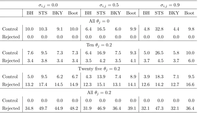
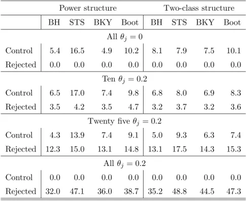
The performance criteria are (1) the empirical FDR compared to the nominal levelα= 0.1; and (2) the empirical power (measured as the average number of false hypotheses rejected). The results are presented in Table 1 (for common correlation) and Table 2 (for power structure and two-class structure). They can be summarized as follows.
• BH, BKY and Boot provide satisfactory control of the FDR in all scenarios. On the other hand, STS is liberal under positive constant correlation and for the power structure scenario.
• For the five scenarios with ten θj = 0.2, BKY is as powerful as BH, while in all other
scenarios it is more powerful. In return, for the single scenario with ten θj = 0.2 under
independence, Boot is as powerful as BKY, while in all other scenarios it is more powerful.
• In the majority of scenarios, the empirical FDR of Boot is closest to the nominal level
α= 0.1.
• STS is often more powerful than Boot but some of those comparisons are not meaningful, namely when Boot provides FDR control while STS does not.
7.2 Robustness of FDR Control against Random Correlations
In the previous subsection, we used three models for the covariance matrix: constant corre-lation, power structure, and two-class structure. In all cases, BH, BKY, and Boot provided satisfactory control of the FDR in finite samples.
The goal of this subsection is to study whether FDR control is maintained for ‘general’ covariance matrices. Since it is impossible to employ all possible covariance matrices in a simulation study, our approach is to employ a large, albeit random, ‘representative’ subset of covariance matrices. To this end, we generate 1,000 random correlation matrices uniformly from the space of positive definite correlation matrices. (Joe (2006) recently introduced a new method which accomplishes this. Computationally more efficient variants are provided by Lewandowski et al. (2007), and we use their programming code which Prof. Joe has graciously shared with us.) We then simulate the FDR for each resulting covariance matrix, taking all standard deviations to be equal to one. However, we reduce the dimension from s = 50 to
s = 4 to counter the curse of dimensionality. Note that an s-dimensional correlation matrix lives in a space of dimension (s−1)s/2. Since we can only consider a finite number of random correlation matrices, we ‘cover’ this space more thoroughly when a smaller value ofsis chosen.
As far as the mean vector is concerned, two scenarios are considered: one θj = 0.2 and one θj = 20. The latter scenario results in perfect power for all four methods.
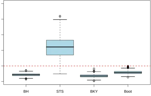
The resulting 1,000 simulated FDRs for each method and each mean scenario are displayed via boxplots in Figure 1. Again, BH, BKY, and Boot provide satisfactory control of the FDR throughout, while STS is generally liberal. In addition, Boot tends to provide FDR control closest to the nominal level α= 0.1, followed by BKY and BH.
We also experimented with a larger value ofsand different fractions of false null hypothe-ses. The results (not reported) were qualitatively similar. In particular, we could not find a constellation where any of BH, BKY, or Boot were liberal.
8
Empirical Applications
8.1 Hedge Fund Evaluation
We revisit the data set of Romano et al. (2008) concerning the evaluation of hedge funds. There are s = 209 hedge funds with a return history of n = 120 months compared to the risk-free rate as a common benchmark. The parameters of interest areθj =µj−µB, whereµj
is the expected return of the jth hedge fund andµB is the expected return of the benchmark.
Since the goal is to identify the funds that outperform the benchmark, we are in the one-sided case (11) with θ0,j = 0, forj= 1, . . . , s.
Naturally, the estimator ofθj is given by
ˆ θn,j = 1 n n X i=1 Xi,j− 1 n n X i=1 Xi,B ,
that is, by the difference of the corresponding sample averages. It is well known that hedge fund returns, unlike mutual fund returns, tend to exhibit non-negligible serial correlations; see, for example, Lo (2002) and Kat (2003). Accordingly, one has to account for this time series nature in order to obtain valid inference. The standard errors for the original data, ˆσn,j, use a
kernel variance estimator based on the prewhitened QS kernel and the corresponding automatic choice of bandwidth of Andrews and Monahan (1992). The bootstrap data are generated using the circular block bootstrap of Politis and Romano (1992), based on B = 5,000 repetitions. The standard errors in the bootstrap world, ˆσ∗n,j, use the corresponding ‘natural’ variance estimator; for details, see G¨otze and K¨unsch (1996) or Romano and Wolf (2006). The choice of the block sizes for the circular bootstrap is detailed in Romano et al. (2008).
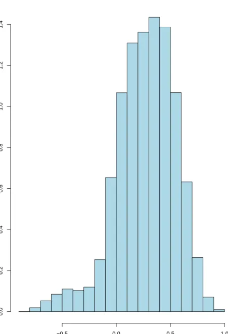
The number of outperforming funds identified by various procedures and for two nominal levels α are presented in Table 3. Both BKY and Boot results in more rejections than BH, with the comparison between BKY and Boot depending on the level. The numbers for STS appear unreasonably high. Apparently, this is due to the fact that the weak dependence (across test statistics) assumption for the application of this method is clearly violated. The median absolute correlation across funds is 0.32; also see Figure 2.
8.2 Pairwise Fitness Correlations
We consider Example 6.5 of Westfall and Young (1993) where the pairwise correlations of seven numeric ‘fitness’ variables, collected from n= 31 individuals, are analyzed. Denote the
s= 72
= 21 pairwise population correlations, ordered in any fashion, byθj, for j = 1, . . . , s, and let ˆθn,j, for j = 1, . . . , s, denote the corresponding Pearson’s sample correlations. Since
the goal is to identify the non-zero population correlations, we are in the two-sided case (12) with θ0,j= 0, for j= 1, . . . , s.
Westfall and Young (1993) provide two sets of individual p-values: asymptotic p-values based on the assumption of a bivariate normal distribution and bootstrapp-values. As can be seen from their Figure 6.4, the two are always very close to each other. However, as pointed out by Westfall and Young (1993, page 194), both sets ofp-values are actually for the stronger null hypotheses of independence rather than zero correlation. Obviously, independence and zero correlation are the same thing for multivariate normal data, but we do not wish to make this parametric assumption.
Instead, we use Efron’s bootstrap to both compute individual p-values and to carry out our bootstrap FDR procedure. (Of course, the same set of bootstrap resamples is used for both purposes.) The details are as follows. The standard errors for the original data, ˆσn,j,
are obtained using the delta method because, again, we do not want to assume multivariate normality; see Example 11.2.10 of Lehmann and Romano (2005b). This results in test statistics
Tn,j =|θn,jˆ |/σn,jˆ . The bootstrap data are generated using Efron’s (1979) bootstrap, based on
B = 5,000 repetitions. The standard errors for the bootstrap data, ˆσ∗
n,j, are computed in
exactly the same fashion as for the original data. This results in bootstrap statistics Tn,j∗ =
|θˆ∗n,j−θˆn,j|/σˆ∗n,j. The individualp-values are then derived according to (4.11) of Davison and
Hinkley (1997): ˆ pn,j = 1 + #{T ∗ n,j ≥Tn,j} B+ 1 . (24)
levels α are presented in Table 4. BKY results in the same number of rejections as BH for both nominal levels. Boot results in the same number of rejections for α = 0.05, but yields three additional rejection forα= 0.1. The numbers for STS again appear unreasonably high.
An alternative way of testingHj :θj = 0 is to reparametrize θj by ϑj = arctanh(θj) = 1 2log 1 +θj 1−θj .
This transformation is known as Fisher’s z-transformation, which under normality is variance stabilizing; see Example 11.2.10 of Lehmann and Romano (2005b). Obviously, θj = 0 if and
only if ϑj = 0. The natural estimator of ϑj is given by ˆϑn,j = arctanh(ˆθn,j). Using the fact
that arctanh′(x) = 1/(1 −x2), the delta method implies the corresponding standard error
˜
σn,j = ˆσn,j/(1−θˆn,j2 ). This results in test statistics Tn,j = |ϑˆn,j|/σ˜n,j. Some motivation for
bootstrapping the z-transformed sample correlation rather than the ‘raw’ sample correlation is given in Efron and Tibshirani (1993, Section 12.6). Again, the bootstrap data are obtained using Efron’s (1979) bootstrap, based on B = 5,000 repetitions. The standard errors for the bootstrap data, ˜σ∗n,j, are computed as ˜σ∗n,j = ˆσn,j∗ /(1−θˆn,j∗ )2. This results in bootstrap statistics Tn,j∗ =|ϑˆ∗n,j −ϑˆn,j|/σ˜n,j∗ . The individual p-values are derived as in (24) again.
The number of non-zero correlations identified by various procedures and for two nominal levels α are also presented in Table 4. While making inference for the ϑj does not necessarily
lead to the same results as making inference for the θj, in particular when the sample sizenis
not large, for this particular data set none of the numbers of rejections change.
9
Conclusion
In this article, we have developed two methods which provide asymptotic control of the false discovery rate. The first method is based on the bootstrap and the second is based on sub-sampling. Asymptotic validity of the bootstrap holds under fairly weak assumptions, but we require an exchangeability assumption for the joint limiting distribution of the test statistics corresponding to true null hypotheses. The method based on subsampling can be justified with-out such an assumption. However, simulations support the use of the bootstrap method under a wide range of dependence. Even under independence, our bootstrap method is competitive with that of Benjamini et al. (2006), and outperforms it under dependence.
The bootstrap method succeeds in generalizing Troendle (2000) to allow for non-normality. However, it would be useful to also consider an asymptotic framework where the number of hypotheses is large relative to the sample size. Future work will address this.
References
Abramovich, F. and Benjamini, Y. (1996). Adaptive thresholding of wavelet coefficients.
Com-putational Statistics & Data Analysis, 22:351–361.
Abramovich, F., Benjamini, Y., Donoho, D. L., and Johnstone, I. M. (2006). Adapting to unknown sparsity by controlling the false discovery rate. Annals of Statistics, 34(2):584– 653.
Andrews, D. W. K. and Monahan, J. C. (1992). An improved heteroskedasticity and autocor-relation consistent covariance matrix estimator. Econometrica, 60:953–966.
Basford, K. E. and Tukey, J. W. (1997). Graphical profiles as an aid to understanding plant breeding experiments. Journal of Statistical Planning and Inference, 57:93–107.
Benjamini, Y. and Hochberg, Y. (1995). Controlling the false discovery rate: A practical and powerful approach to multiple testing. Journal of the Royal Statistical Society, Series B, 57(1):289–300.
Benjamini, Y. and Hochberg, Y. (2000). On the adaptive control of the false discovery rate in multiple testing with independent statistics. Journal of Educational and Behavioral Statis-tics, 25(1):60–83.
Benjamini, Y., Krieger, A. M., and Yekutieli, D. (2006). Adaptive linear step-up procedures that control the false discovery rate. Biometrika, 93(3):491–507.
Benjamini, Y. and Liu, W. (1999). A stepdown multiple hypotheses testing procedure that controls the false discovery rate under independence. Journal of Statistical Planning and
Inference, 82:163–170.
Benjamini, Y. and Yekutieli, D. (2001). The control of the false discovery rate in multiple testing under dependency. Annals of Statistics, 29(4):1165–1188.
Davison, A. C. and Hinkley, D. V. (1997). Bootstrap Methods and their Application. Cambridge University Press, Cambridge.
Drigalenko, E. I. and Elston, R. C. (1997). False discoveries in genome scanning. Genet
Epidemiol, 15:779–784.
Efron, B. (1979). Bootstrap methods: Another look at the jackknife. Annals of Statistics, 7:1–26.
Efron, B. and Tibshirani, R. J. (1993). An Introduction to the Bootstrap. Chapman & Hall, New York.
Genovese, C. R. and Wasserman, L. (2004). A stochastic process approach to false discovery control. Annals of Statistics, 32(3):1035–1061.
G¨otze, F. and K¨unsch, H. R. (1996). Second order correctness of the blockwise bootstrap for stationary observations. Annals of Statistics, 24:1914–1933.
Hommel, G. and Hoffman, T. (1988). Controlled uncertainty. In Bauer, P., Hommel, G., and Sonnemann, E., editors, Multiple Hypthesis Testing, pages 154–161. Springer, Heidelberg. Joe, H. (2006). Generating random correlation matrices based on partial correlations. Journal
of Multivariate Analysis, 97:2177–2189.
Kat, H. M. (2003). 10 things investors should know about hedge funds. AIRC Working Paper 0015, Cass Business School, City University. Available at http://www.cass.city.ac.uk/airc/papers.html.
Lahiri, S. N. (1992). Edgeworth correction by ‘moving block’ bootstrap for stationary and nonstationary data. In LePage, R. and Billard, L., editors,Exploring the Limits of Bootstrap, pages 183–214. John Wiley, New York.
Lahiri, S. N. (2003). Resampling Methods for Dependent Data. Springer, New York.
Lehmann, E. L. and Romano, J. P. (2005a). Generalizations of the familywise error rate.
Annals of Statistics, 33(3):1138–1154.
Lehmann, E. L. and Romano, J. P. (2005b). Testing Statistical Hypotheses. Springer, New York, third edition.
Lewandowski, D., Kurowicka, D., and Joe, H. (2007). Generating random correlation ma-trices based on vines and extended Onion method. Preprint, Dept. of Mathematics, Delft University of Technology.
Lo, A. W. (2002). The statistics of Sharpe ratios. Financial Analysts Journal, 58(4):36–52. Mehrotra, D. V. and Heyse, J. F. (2004). Use of the false discovery rate for evaluating clinical
safety data. Statistical Methods in Medical Research, 13:227–238.
Politis, D. N. and Romano, J. P. (1992). A circular block-resampling procedure for stationary data. In LePage, R. and Billard, L., editors,Exploring the Limits of Bootstrap, pages 263– 270. John Wiley, New York.
Politis, D. N. and Romano, J. P. (1994). The stationary bootstrap. Journal of the American
Statistical Association, 89:1303–1313.
Politis, D. N., Romano, J. P., and Wolf, M. (1999). Subsampling. Springer, New York. Reiner, A., Yekutieli, D., and Benjamini, Y. (2003). Identifying differentially expressed genes
using false discovery rate controlling procedures. Bioinformatics, 19:368–375.
Romano, J. P. and Shaikh, A. M. (2006a). On stepdown control of the false discovery propor-tion. In Rojo, J., editor,IMS Lecture Notes—Monograph Series, 2nd Lehmann Symposium—
Optimality, pages 33–50.
Romano, J. P. and Shaikh, A. M. (2006b). Stepup procedures for control of generalizations of the familywise error rate. Annals of Statistics, 34(4):1850–1873.
Romano, J. P., Shaikh, A. M., and Wolf, M. (2008). Formalized data snooping based on generalized error rates. Econometric Theory, 24(2):404–447.
Romano, J. P. and Wolf, M. (2006). Improved nonparametric confidence intervals in time series regressions. Journal of Nonparametric Statistics, 18(2):199–214.
Romano, J. P. and Wolf, M. (2007). Control of generalized error rates in multiple testing.
Annals of Statistics, 35(4):1378–1408.
Sarkar, S. K. (2002). Some results on false discovery rate in stepwise multiple testing proce-dures. Annals of Statistics, 30(1):239–257.
Storey, J. D., Taylor, J. E., and Siegmund, D. (2004). Strong control, conservative point estimation and simultaneous conservative consistency of false discovery rates: A unified approach. Journal of the Royal Statistical Society, Series B, 66(1):187–205.
Troendle, J. F. (2000). Stepwise normal theory test procedures controlling the false discovery rate. Journal of Statistical Planning and Inference, 84(1):139–158.
van der Laan, M. J., Dudoit, S., and Pollard, K. S. (2004). Augmentation procedures for control of the generalized family-wise error rate and tail probabilities for the proportion of false positives. Statistical Applications in Genetics and Molecular Biology, 3(1):Article 15. Available at http://www.bepress.com/sagmb/vol3/iss1/art15/.
Westfall, P. H. and Young, S. S. (1993). Resampling-Based Multiple Testing: Examples and
Williams, V. S. L., Jones, L. V., and Tukey, J. W. (1999). Controlling error in multiple com-parisons, with examples from state-to-state differences in educational achievement. Journal
of Educational and Behavioral Statistics, 24(1):42–69.
Yekutieli, D. and Benjamini, Y. (1999). Resampling-based false discovery rate controlling multiple test procedures for correlated test statistics. Journal of Statistical Planning and
Table 1: Empirical FDRs expressed as percentages (in the rows “Control”) and average number of false hypotheses rejected (in the rows “Rejected”) for various methods, with n = 100 and
s = 50. The nominal level is α = 10%. The number of repetitions is 5,000 per scenario and the number of bootstrap resamples is B = 500.
σi,j = 0.0 σi,j = 0.5 σi,j = 0.9
BH STS BKY Boot BH STS BKY Boot BH STS BKY Boot Allθj = 0 Control 10.0 10.3 9.1 10.0 6.4 16.5 6.0 9.9 4.8 32.8 4.4 9.8 Rejected 0.0 0.0 0.0 0.0 0.0 0.0 0.0 0.0 0.0 0.0 0.0 0.0 Tenθj = 0.2 Control 7.6 9.5 7.3 7.3 6.4 16.9 7.5 9.3 5.0 26.5 5.8 10.0 Rejected 3.4 3.8 3.4 3.4 3.5 4.2 3.5 4.1 3.7 4.5 3.7 6.0 Twenty fiveθj = 0.2 Control 5.0 9.5 6.2 6.7 4.3 13.9 7.4 8.9 3.9 18.3 7.1 9.5 Rejected 13.2 17.4 14.5 14.9 12.3 15.1 13.1 14.1 12.6 14.2 12.7 16.6 All θj = 0.2 Control 0.0 0.0 0.0 0.0 0.0 0.0 0.0 0.0 0.0 0.0 0.0 0.0 Rejected 34.8 49.7 44.9 48.2 31.9 46.9 36.4 39.1 32.1 47.3 32.1 36.4
Table 2: Empirical FDRs expressed as percentages (in the rows “Control”) and average number of false hypotheses rejected (in the rows “Rejected”) for various methods, with n = 100 and
s = 50. The nominal level is α = 10%. The number of repetitions is 5,000 per scenario and the number of bootstrap resamples is B = 500.
Power structure Two-class structure BH STS BKY Boot BH STS BKY Boot
All θj = 0 Control 5.4 16.5 4.9 10.2 8.1 7.9 7.5 10.1 Rejected 0.0 0.0 0.0 0.0 0.0 0.0 0.0 0.0 Ten θj = 0.2 Control 6.5 17.0 7.4 9.8 6.8 8.0 6.9 8.3 Rejected 3.5 4.2 3.5 4.7 3.2 3.7 3.2 3.6 Twenty fiveθj = 0.2 Control 4.3 13.9 7.4 9.1 5.0 9.3 6.3 7.4 Rejected 12.3 15.0 13.1 14.8 13.1 17.5 14.3 15.3 All θj = 0.2 Control 0.0 0.0 0.0 0.0 0.0 0.0 0.0 0.0 Rejected 32.0 47.1 36.0 38.7 35.2 48.8 44.5 47.3
Table 3: Number of outperforming funds identified. Procedure α= 0.05 α= 0.1
BH 58 101
STS 173 203
BKY 72 142
Boot 81 129
Table 4: Number of non-zero correlations identified. Procedure α= 0.05 α= 0.1
BH 2 4
STS 10 20
BYK 2 4
BH STS BKY Boot 0.05 0.10 0.15 0.20 0.25 0.30
Realized FDRs: one theta = 0.2
BH STS BKY Boot 0.05 0.10 0.15 0.20 0.25 0.30
Realized FDRs: one theta = 20
Figure 1: Boxplots of the simulated FDRs described in Subsection 7.2. The horizontal dashed lines indicate the nominal level α= 0.1.
Histogram of cross correlations Cross correlation Density −0.5 0.0 0.5 1.0 0.0 0.2 0.4 0.6 0.8 1.0 1.2 1.4
Figure 2: Histogram of the 208·209/2 = 21,736 cross correlations between the excess returns of the 209 hedge funds. Since it is not true that the majority of these correlations are close to zero, the weak dependence assumption of Storey et al. (2004) is clearly violated.