Authorship Identification and Writeprint Visualization

(1)

AUTHORSHIP IDENTIFICATION AND WRITEPRINT

VISUALIZATION

STEVENH. H. DING

A THESIS IN

THE CONCORDIAINSTITUTE FORINFORMATIONSYSTEMSENGINEERING

PRESENTED INPARTIALFULFILLMENT OF THEREQUIREMENTS

FOR THEDEGREE OF MASTER OFAPPLIED SCIENCE ININFORMATIONSYSTEMS SECURITY

CONCORDIA UNIVERSITY MONTRÉAL, QUÉBEC, CANADA

APRIL2014

(2)

C

ONCORDIA

UNIVERSITY

School of Graduate Studies

This is to certify that the thesis prepared

By: Steven H. H. Ding

Entitled: Authorship Identification and Writeprint Visualization

and submitted in partial fulfillment of the requirements for the degree of

Master of Applied Science in Information Systems Security

complies with the regulations of this University and meets the accepted standards with re-spect to originality and quality.

Signed by the final examining committee:

Dr. Chadi Assi Chair

Dr. Amr Youssef CIISE Examiner Dr. Peter Grogono External Examiner Dr. Benjamin C. M. Fung Supervisor

Dr. Mourad Debbabi Supervisor Approved by

Chair of Department or Graduate Program Director 20

(3)

Abstract

Authorship Identification and Writeprint Visualization

Steven H. H. Ding

The Internet provides an ideal anonymous channel for concealing computer-mediated malicious activities, as the network-based origins of critical electronic textual evidence (e.g., emails, blogs, forum posts, chat log etc.) can be easily repudiated. Authorship at-tribution is the study of identifying the actual author of the given anonymous documents based on the text itself, and, for decades, many linguistic stylometry and computational techniques have been extensively studied for this purpose. However, most of the previous research emphasizes promoting the authorship attribution accuracy and few works have been done for the purpose of constructing and visualizing the evidential traits; also, these sophisticated techniques are difficult for cyber investigators or linguistic experts to inter-pret. In this thesis, based on the EEDI (End-to-End Digital Investigation) Framework we propose a visualizable evidence-driven approach, namely VEA, which aims at facilitating the work of cyber investigation. Our comprehensive controlled experiment and stratified experiment on the real-life Enron email data set both demonstrate that our approach can achieve even higher accuracy than traditional methods; meanwhile, its output can be easily visualized and interpreted as evidential traits. In addition to identifying the most plausible

(4)

author of a given text, our approach also estimates the confidence for the predicted result based on a given identification context and presents visualizable linguistic evidence for each candidate.

(5)

Acknowledgments

I would like to express my deepest gratitude to my supervisor, Dr. Benjamin C. M. Fung, for his experienced guidance, constructive criticism, and persistent support on me through-out the research. He has been a tremendous mentor for me. His encouragement and advices on both my research and career, which enables me to grow as a researcher, have been price-less.

I also would like to express my sincere appreciation to my supervisor, Dr. Mourad Deb-babi, for his patience, confidence, and continuous support on me to complete this research and thesis. He provides a great source of opportunities and encouragement. I am deeply grateful to him.

My sincere appreciation also goes to all the faculty members and staff of Concordia Institute for Information Systems Engineering. In addition, I am very grateful toConcordia Universityfor giving me this opportunity to study and work.

Last but not least, I would like to express my boundless appreciation from the button of my heart to my warm family for their irreplaceable and unconditional love. Moreover, special thanks to my fiancée, Lynne, for accompanying me, also for her firm support and heartfelt understanding.

(6)

“The painter has the Universe in his mind and hands.” - Leonardo da

(7)

To my parents and

(8)

List of Figures

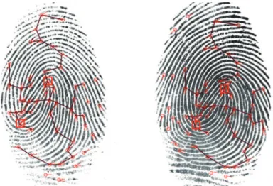
1 A sample fingerprint minutiae matching diagram generated by using fin-gerprint software and data fromNEUROtechnology1. . . 6 2 Examples of spectrum-based information-gain-inspired writeprint

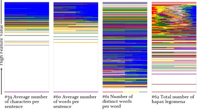
visual-ization scheme. Different color represents writing style of different candi-date author. Spectrum value represents ascending feature value. . . 22 3 Examples of box-plot-based writeprint visualization scheme. Different

colour (series on the diagram) stands for different candidate authors’ pre-vious writing sampleM_i. . . 23 4 Overview of VEA in EEDI framework. . . 26 5 A sample 3-gram space. . . 32 6 Evidentiary chain visualization: hypothesis representations and the

visual-ized evidence units. . . 40 7 Cumulative evidence unit scoring diagram: the serial that achieves the

highest score at the end of x-axis is for the most plausible candidate. . . 46 8 The architect design of the forensic software for authorship analysis. . . 48

(11)

10 Dataset analysis. . . 53 11 Performance comparison between isolated events. For all the diagrams, the

upper surface is lexicaln-gram event, the intermediate surface is character n-gram event and the lowest surface is POSn-gram event. . . 56 12 Performance comparison between approaches. For all the diagrams, the

upper surface is VEA, the intermediate surface is the stylometric J48 and the intermediate surface is the stylometric SVM. . . 58 13 Performance comparison between VEA, voting ensemble, and lexical

n-gram event. X axis indicates different scenario, for example2-120stands for a 2 candidates scenario with 120 writing samples for each of them. Y axis indicates the identification accuracy. . . 61 14 Performance of VEA on unbalanced-class problem. . . 63

(12)

List of Tables

1 Static features summarized from [IBFD10]. . . 18

2 Identification accuracy using different models. . . 20

3 Employed lingusitic features. . . 28

4 Features for confidence estimation (identification context) . . . 35

5 Confidence estimation. . . 47

6 Employed stylometric features. . . 60

(13)

Chapter 1 Introduction

Research in authorship attribution on anonymous documents is experiencing a continu-ing exponential growth in recent years because a reliable authorship attribution technology is useful and valuable in many fields: literary science, sociolinguistic research, Psycholin-guistics, social psychology, forensics, and medical diagnosis, etc. [Dae13] Especially under the globalized and decentralized nature of the Internet, the communications of malicious activities (e.g., illegal material distribution, ransom, and harassment, etc. [AC08, IBFD13]) can be easily hidden or repudiated. Authorship analysis techniques are capable of delving into the information from different linguistic levels and of identifying the textual identity trace, which potentially greatly facilitates the work of cyber forensic investigators and sus-tains the social accountability. Stylometry even has been employed as evidence in a law court [BAG12].

(14)

The study of authorship attribution has a long-standing history [MW64] and many lin-guistic stylometry and computational techniques have been developed for solving this prob-lem. These methods have demonstrated outstanding effectiveness in identifying the actual authors; however, those techniques that achieve the highest accuracy always involve sophis-ticated, obscure computational models [Sta09]. These models as black-box approaches can hardly be interpreted by an investigator and their output is too simple to use as evidence in a court of law.

These issues handicap traditional methods from being widely applied to the real-life lawsuits as convincing evidence. Practically, computational stylometry is calling for ‘more explanation as opposed to purely quantitative measure’ [Dae13]. A better approach should provide explainable and presentable convincing traces as evidence.

Most of the previous research did not measure the degradation of their methods’ perfor-mance as the quantity/quality of the available information degraded simultaneously, which is also noted by [Sol13]. These models are mostly evaluated only on formal writings, which are relatively long, informative, well-structured, and free from grammatical errors. On the contrary, short snippets are relatively casual, and their stylometric features have larger variation. As shown in recent research [KSA11, LD11, NPG+12], authorship attri-bution accuracy is greatly and directly affected by many objective factors (e.g., text length, number of known author samples, etc.) due to the unstructured nature of the text itself. It is critical for authorship analysis researchers to conduct attribution evaluation experiments in varying attribution scenarios in order to ‘exclude a bogus conclusion based on inadequate

(15)

In this thesis, we present a visualizable evidence-driven approach, namely VEA, for the purpose of facilitating the work of cyber investigation and the decision-making pro-cess in a law court. Our approach is driven by evidence and based on the lazy learning scheme [NPG+12]. Basically, our method searches inside the anonymous document for all the writing styles of different linguistic modalities as evidence and matches them to the pre-built candidate profiles. Evidence from different linguistic modalities are combined by using confidence estimation. Finally, it visualizes all the evidence on the given hypotheses, and it is able to present a visual discrimination between hypotheses. Besides, it also pro-vides an estimated confidence value based on the quality of the evidence and the amount of available information in a given attribution scenario. More importantly, we modeled the attribution scenario and conducted our experiments in varying situations (i.e., varying length of text, varying candidate size, etc.) to fully evaluate our method.

1.1 The problem

In the authorship attribution problem, a set of candidate authors, along with their corre-sponding individual writing samples, are available, and the task is to identify the most plausible author among these candidates based on the given anonymous document [MW64, Hol98, IBFD13]. In most of the previous studies, the candidate sets involved in their sce-narios are mostly of size ranging from 2 to 20. Although the size of a real-life candidate set may scale up to more than ten thousand, it is more appropriate to first employ scalable methods from [KSA11] or [NPG+12] to determine a potential candidate subset, and then

(16)

use other relatively more accurate techniques to figure out the most plausible conclusion. An open-set authorship attribution problem is a variant of the original authorship attri-bution problem [KSA11]. In this research problem, the solution is allowed to output an alternative “unknown” option to indicate that the actual author could not be found or deter-mined from the given candidate set based on presented available information. In fact, any solutions that are capable of outputting a monotonous probability indicating the confidence of a predicted result can be applied to this problem by setting an appropriate threshold on this output probability value.

We formally define the authorship identification problem with a probability confidence value output, as mentioned above. To be consistent in terminology, in this thesis “can-didates” or “candidate authors” refer to the potential authors of the anonymous message, and “author” or “actual author” refer to the true author of the anonymous message. Let C = {C1, C2, . . . , CN} be a set ofN candidate authors andM = {M1, M2, ..., MN} be

a set of their corresponding writing samples whereMi denotes the set of known samples

authored byCi. The task is to identify the actual author of given anonymous snippetωfrom

the candidate setC based on the information available inM. Furthermore, the algorithm should be able to output a probability valuep∈ [0,1], which denotes the algorithm’s con-fidence in its predicted result on the given problem context:p= 0indicates an completely uncertain result, whilep= 1indicates a very confident result.

(17)

1.2 Challenges and Contributions

The authorship attribution problem is similar to the text classification problem. The plain text classification task is tough inherently due to unstructured nature of textual data. By unifying the feature vector and extracting the vector for each sample text, the textual data can be transformed into structured samples, which is the typical and traditional authorship attribution solution [Hol94, Sta09]. However, the deviation of each element inside the vec-tor is still strongly affected by the length of available text. Online texts are mostly very short and, therefore, contain limited information about the writing style [IBFD13], which causes a larger fluctuation around the mean value in the unified feature vector. This introduces difficulties in achieving higher accuracy due to the presence of more outliers.

In order to retain reasonable accuracy in the identification task, we try to maximize the information gained from the given anonymous document and combine both statistical similarity and data mining techniques to develop a hybrid model using the lazy learning mechanism. Specifically, our contributions are summarized as follows:

• To the best of our knowledge, this is the first trial to design an authorship attribu-tion approach with the goal of promoting not only the accuracy measure, but also the interpretability and the visualizability of the predicted result. From the very be-ginning this approach is designed from the perspective of collecting evidence. We systematically outlined our approach by employing the EEDI (End-to-End Digital Investigation) framework [BKW12], one of the recognized forensic processes used

(18)

Figure 1: A sample fingerprint minutiae matching diagram generated by using fingerprint software and data fromNEUROtechnology1_.

in digital forensics investigations. By doing this, we are able to construct a cumula-tive evidentiary effect supporting the final output result, and the construction process can be easily explained using the EEDI framework.

• Our approach is concise in design, and its output is visualizable. Inspired by the visualization of fingerprint matching1in Figure 1, where the correlations among fin-gerprint minutiae can be visually compared, rather than presenting a simple numeric result we devise an approach visualizing all the supporting evidence on top of our visual representation of hypotheses. We are able to present a visual discrimination among these hypotheses and present detailed supporting evidence. More importantly, we systematically conducted our experiments under varying authorship attribution scenarios in order to fully evaluate our approach. Our experiments demonstrate that our approach achieves the state-of-the-art attribution accuracy, while the output evi-dence is visualizable, presentable, and explainable.

(19)

• Based on the specific context of the given authorship attribution problem, our ap-proach is also able to estimate a confidence value and, thus, can be applied to the authorship open-set problem. Based on those scenario-related features that we iden-tified, our method can accurately model and predict the final classification accuracy. Moreover, to our best knowledge and differing from previously employed voting-based ensemble methods such as [KSA11], it is the first trial to combine multiple classifiers by normalizing their scoring vector using individually estimated confi-dence values on given classification contexts. We consider classifiers built on fea-tures of different linguistic modalities separately. We explain the necessity of this step by arguing that stylistic features from different linguistic modalities have differ-ing capacity in determindiffer-ing the actual author and varydiffer-ing sensitivity to the objective conditions in a given scenario. This is due to the unpredictable coherence of writing style among known authors’ sample writings, and it is in accordance with our ob-servations in the experiments. In addition, our approach is extensible, where other features from different linguistic modalities or non-linguistic features can be further added as additional events.

1.3 Thesis Organization

The rest of this thesis is organized as follows: Chapter 2 reviews and discusses recent development and issues in authorship analysis. Chapter 3 presents our analysis on static stylometry. Chapter 4 elaborates ourVisualizable Evidence-driven Approachof authorship

(20)

attribution in detail. Chapter 5 evaluates our proposed methodVEAon the Enron real-life dataset. Chapter 6 concludes this thesis.

(21)

Chapter 2 Related Works

The history of authorship attribution backed up by computational and statistical methods can be dated from the 19th century [Sta09]. Contributions to this area can be broadly cat-egorized from three aspects: the involved stylometric features, the employed attribution techniques, and the attacks against authorship attribution techniques. Previous research mainly focuses on promoting quantitative evaluation and few have been done for visual-ization or explanation. Most explanations for the choice of features and algorithmic pa-rameters are simply driven by the classification accuracy. In this chapter we are going to discuss several recent related works and research trends in authorship analysis research. An inclusive survey on the complete history is beyond the scope of this work. Broader comprehensive surveys can be referred to [Hol94, Juo06, Sta09].

(22)

2.1 Stylometric Features

Stylometry is the solution of authorship recognition by investigating the linguistic char-acteristics inside the given text document, and stylometric features are those linguistic marks that could qualify or quantify these linguistic characteristics [Sta09, BAG12]. Sty-lometric features can be categorized into different linguistic levels [Dae13, Sta09], or, more precisely, linguistic modalities [SSMyR13, SPRMy11]. Various features of differ-ent modalities have demonstrated their effectiveness in distinguishing human writing pat-terns. These modalities include lexical [KSA06, Hal07, Sav12], character-based [KSA11, KSAW12, ESMy11], syntactic [KKW+11, SVS+13, RKM10], semantic [HS11, SZB11, SBZ12] and application-specific modality [CRS+12].

Among all these stylometric features, the charactern-gram modelin character-based linguistic modality performs the best, and it is comparatively more robust against the oth-ers [LD11, KSA11]. The character n-gram model actually captures information cross-ing different modalities [HS06]; for example, a frequent ‘ed’ bigram in a character-based modality may also carry the frequent usage of past tense in a syntactic modality. However, as pointed out in [NPG+12], solutions using these features also take the risk of capturing the context rather than the authors’ writing style. Regarding the relationship between sty-lometric modalities, [SSMyR13] employed the word “orthogonal” to assimilate them as independent components. In fact, this word appears to be over-dramatic because correla-tions among modalities do exist. For example, some functional words in lexical modality have exactly one corresponding Part-of-Speech tag in the syntactic modality (e.g., ‘to’ to

(23)

POS tag ‘TO’). We argue that correlations may exist among linguistic modalities, but they have differing capacity in attributing the correct author based on the given problem context. Stylometric feature sets involved in previous studies can also be divided into two groups: the unified feature set and the distinct feature set. Under the unified feature set, which is employed by most previous solutions, every candidate is modeled using the same set of fea-tures; however, under the distinct feature set, candidates are given different feature sets. As shown by [AC08] and [IBFD13], the distinct algorithmic feature set can better distinguish among candidates’ writing styles and achieve higher performance.

2.2 Attribution Techniques

After the selection of the specific feature scheme, attribution techniques are employed to predict the actual author of a given snippet. Attribution techniques can be divided into a similarity-based approach [PSWK03, Hal07, KSA11] and a machine-learning-based ap-proach [SG06, LV09]. The similarity-based apap-proach employs distance functions [Sav12] to quantify the similarity between a candidate profile and a given anonymous document, while the machine-learning-based approach builds complicated models to classify the given document. Those solutions that have the best performance on benchmark data sets are mostly machine-learning related.1 _{Among the machine-learning-based approaches, the} SVM-based approach [AC08] and the association-rule-based approach [IBFD13] achieve higher accuracy due to the fact that they both consider the combination of feature values among the high-dimensional space. Other machine-learning techniques are also employed,

(24)

involving decision tree, Artificial Intelligence [TSH96], and clustering [LWD13]. Typ-ically, one-versus-all SVM is chosen as the standard method when comparing different stylometric features because it has a better multi-class classification capacity [DK05].

Even though a machine-learning-related approach can achieve a higher quantitative per-formance, most involve a complicated computational model, and it is difficult to interpret its decision-making process. The similarity-based approach is much easier to visualize and interpret because it retains a monotonous linear relationship between evidence and conclu-sion: the smaller the distance between author profile and the targeted document, the more similar writing styles they possess.

2.3 Ensemble Method

Recent studies in authorship analysis demonstrate a trend of employing ensemble meth-ods to combine several separately trained classifiers due to the fact that multiple classifiers can better fit into sample data and boost the attribution accuracy. In [KSA11], multiple classifiers are built based on different feature sets that are randomly selected from all avail-able space-free character 4-grams, and the final output depends on their votes. In [KS11], a co-training approach is employed by using two classifiers. Also, in [RKM10], higher performance is achieved by employing the votes from classifiers built on different feature sets.

(25)

classification contexts (e.g., the length of an anonymous snippet, candidate score distribu-tion, training size, etc.), classifiers built by using features of varying linguistic modalities will have varying capacity to attribute the author correctly. It is more rational to weight them accordingly: under the specific classification context, the one that can better discrim-inate writing style should be weighted more. In our approach, each classifier is built based on features from different linguistic modalities, and it is weighted based on its demonstrated consistency among prior written samples.

2.4 Adversary Stylometry

From the perspective of the adversary, several studies are trying to circumvent authorship attribution techniques [KG06, JV10, BAG12]. The most influential study is by [BAG12]. They conducted an experiment on the effectiveness of stylometry obfuscation and imitation. By recruiting volunteers and using the Amazon Mechanical Turk2 platform, they asked participants to submit their prior written samples and then write an imitation passage and an obfuscation passage (no guideline was given to participants on how to obfuscate or imitate). Their results demonstrate that there is a significant drop in identification accuracy when it comes to these attacks. Also the accuracy drops when it comes to one-step, two-step translation attacks.

However, their experimental setup may not truly reflect the effectiveness of their obfus-cating approach. First, the decrease in identification accuracy is mostly caused by the mis-match of context between the obfuscated passages and the training passages. Obfuscated

(26)

passages are about the description of participants’ neighbours while pre-existing writing samples are mostly “scholarly”, and thus more formal. Second, their experiment also com-bined and split passages to generate known author writing samples, which may also lead to a high contextual correlation among samples. As we know, word-level tokens are good at capturing contextual and thematic correlation [FWE03]. We ran our model based on pure lexicaln-gram on their data set and it showed a high correlation of word-leveln-gram among training samples (86.01% identification accuracy for 45 authors; around 500 tokens per sample), with a low correlation between obfuscated texts and training texts. Also in the study of [Juo12], a method for detecting the obfuscated texts is proposed using charac-ter 3-grams and word 3-grams. Their experiments also demonstrated a large difference in gram usage between pre-existing samples and obfuscated samples. The difference in the gram usage pattern implies the contextual and thematic variations, which naturally leads to the unsatisfactory result when it comes to authorship attribution techniques that employ character bigrams and trigrams.

2.5 Attribution Result and Result Visualization

Most of the aforementioned studies simply display the most plausible candidate as their output result. Some recent research is able to add an estimated value indicating the attri-bution confidence [KSA11, NPG+12]. However, due to the fact that authorship analysis techniques are not reliable enough to be widely recognized, this kind of simple output will

(27)

still raise doubts when applied in real-life cases. Instead, visualized evidence corroborat-ing why this candidate author is selected to be the most plausible one will be more help-ful. The only work that we found on formally visualizing attribution output is by [AC06]. Nonetheless, their coordinate graph-based visual representation of the output result is still too abstract from the intuitive linguistic characteristics.

(28)

Chapter 3 Analysis of Static Stylometry

In this chapter, we present our study of the static stylometric features regarding its effec-tiveness when employed with the similarity-based models for authorship attribution. Firstly we discuss the schemes for data representation and analyze the distance functions, which quantify the proximity among individual candidate writing styles in the similarity-based solutions for authorship identification. After that we present two visualization methods for analyzing the variation of writing styles among candidate authors. In the end we discuss their capacities and limitations.

As shown by the following discussion, the similarity-based approaches with static sty-lometric feature set cannot achieve higher identification accuracy than the state-of-the-art identification techniques such as [IBFD13]. Moreover, diagram-based visualization scheme for static stylometric features can be easily interpreted and it is useful for the pur-pose of feature analysis. However, to visualize the writeprint for authorship identification, it fails to consider the combination of different stylometric features and in each case the

(29)

number of diagrams for user to inspect is overwhelming.

3.1 Static Stylometry and Data Representation

As mentioned in Chapter 2, stylometric features can be categorized based on their linguistic properties, more precisely, linguistic modalities. However, based on their representations, these features can also be divided intostatic featuresanddynamic features[LWD12]. Static features are chosen before the training phase, and they are independent to the dataset, while dynamic features are chosen as part of the training process [LWD12]. For example, the av-erage length of sentences is a static feature, and the frequency value of the most frequent noun in the training corpus is a dynamic feature. To solve the problem defined in Sec-tion 1.1, initially we consider employing the static stylometric features which have been predominantly adopted in previous studies [AC08, Sta09, NPG+12, BAG12, IBFD13] until very recently [KSA11, LWD12].

In the literature of stylometry, lots of features have been developed for the purpose of modeling writing styles [Juo06, ZLCH06, Sta09]. We summarize the static stylometric features in [IBFD10] and list them in Table 1. These features cover character level modality, lexical level modality and syntactic modality. As shown in Table 1, all of these static features are of type numeric and are calculated using the frequency value or ratio value. They model the preference and behavior of an individual on using specific vocabulary and grammatic structures in his/her writings. These features have demonstrated accurate authorship identification in varying settings [AC08, BAG12, IBFD13].

(30)

Table 1: Static features summarized from [IBFD10]. Features type Features

Character features 1. Character count (P) (character-based) 2. Ratio of digits to P

3. Ratio of letters to P

4. Ratio of uppercase letters to P 5. Ratio of spaces to P

6. Ratio of tabs to P

7. Occurrences of alphabets (A-Z) (26 features)

8. Occurrences of special characters: <>%|{}. . .(21 features) Lexical features 1. Token count(T)

(word-based) 2. Average sentence length in terms of characters 3. Average token length

4. Ratio of characters in words to P

5. Ratio of short words (1-3 characters) to T

6. Ratio of word length frequency distribution to T (20 features) 7. Ratio of types to T

8. Vocabulary richness (Yule’s K measure) 9. Hapax legomena

10. Hapax dislegomena

Syntactic features 1. Occurrences of punctuations and function words (311 features).

To represent a snippet as a numeric vector using these predefined features, there are two major approaches. The first approach is to treat each snippet as a standalone sample, and the vector for this sample is calculated independently using predefined features. In this case, there are|M_i|samples for candidate authorC_i.

The second approach treats all the snippets written by one specific author as a text corpus, and only one vector vectorCi _{is calculated for each author. In this case, there}

is no need to combine vectors of written snippets for deriving a final representation for writing style. We analyze both of these two approaches and discuss their performance in the following section.

(31)

3.2 Similarity-based Approach and Distance Functions

As mentioned in Chapter 2, attribution techniques are employed to predict the most plau-sible author after representing text snippets as numeric vectors. In this section, we analyze similarity-based approach which employs distance functions to quantify the similarity be-tween anonymous snippet and candidate authors’ writing style, due to the fact that data mining related techniques, such as SVM, introduce complicated computational models and thus they can be hardly visualized.

For the first approach of data representation, each candidate author has|M_i|vectors. To derive a final vector for candidate authorCi, the typical mean center vector is employed:

vectorCi ₌ 1

|Mi|

PMi

docvectordoc. For the second data representation approach, this step is

unnecessary since each candidate already has one dedicated vectorvectorCi_.

Assuming that we have SF static features in total, to quantify the proximity between vectorCi _and _vectorω _{for anonymous snippet} _{ω, we consider following typical distance}

functions: • Euclidean distance: dist(vectorCi_{, vector}ω_{) =} v u u t SF X k=1 (vectorCi k −vectorkω)2 • Cosine distance:

dist(vectorCi_{, vector}ω_{) =} vectorCi·vectorω |vectorCi_{| × |}_vectorω_| • Pearson distance: dist(vectorCi_{, vector}ω_{) = 1}₋ 1 SF SF X k=1 (vector Ci k −vectorCi σ_vectorCi )(vector ω k −vectorω σvectorω )

(32)

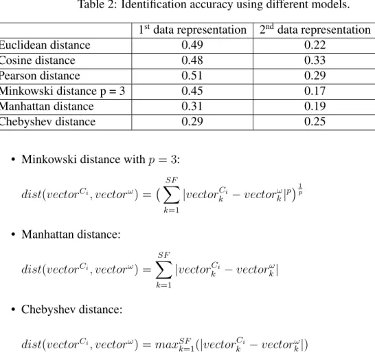
Table 2: Identification accuracy using different models. 1st_{data representation} ₂nd_{data representation}

Euclidean distance 0.49 0.22 Cosine distance 0.48 0.33 Pearson distance 0.51 0.29 Minkowski distance p = 3 0.45 0.17 Manhattan distance 0.31 0.19 Chebyshev distance 0.29 0.25

• Minkowski distance withp= 3: dist(vectorCi_{, vector}ω_{) =} SF X k=1 |vectorCi k −vector ω k|p 1_p • Manhattan distance: dist(vectorCi_{, vector}ω_{) =} SF X k=1 |vectorCi k −vector ω k| • Chebyshev distance:

dist(vectorCi_{, vector}ω_{) =}_maxSF

k=1(|vector

Ci

k −vectorωk|)

To analyze the effectiveness of aforementioned data representations and distance func-tions for the task authorship identification, we randomly sampled three scenarios where 10 candidates are involved from the Enron email dataset. We tested the combination of aforementioned data representations and distance function using 10-fold cross validation, and used the identification accuracy (ratio of samples that are correctly identified) as our evalution measure. The test result is listed in Table 2.

This small analytical test is by no mean inclusive and comprehensive, but it turns out that the second data representation, which considers each writing snippet as independent sample, outperforms the first representation. Also theP earson distanceappears to at best

(33)

model the writing styles. However,51% identification accuracy still is incomparable with other state-of-the-art identification approaches such as [IBFD13].

3.3 Analysis through Visualization

In this section, we present two visualization schemes for static stylometric analysis. The first scheme is spectrum based approach, which is inspired from theinformation gain the-ory. Four examples are shown in Figure 2, respectively based on the static feature described below the diagram. In this visual representation scheme, the spectrum stands for the as-cending feature value, and different colour stands for writing style for different candidate author. For example, in the first diagram on the left, colour blue mostly gathers in the upper area on spectrum, and this indicates that the candidate author corresponding to colour blue demonstrates high number of characters per sentence in his previous writing samples. Each horizontal line on the spectrum stands for the demonstrated usage on this specific value. If the colour of this line is purely only one specific colour, it means that this specific value on this feature is only revealed on the writing samples of the candidate author corresponding to this colour. For example, if a horizontal line is separated into two parts of equal length with different colour, it means that this specific value on this feature is demonstrated equally in the writing samples of these two candidate authors.

To calculate each line, we apply Equation 1 for each candidate author. f stands for feature type,f vstands for the given specific feature value,Lstands for the spectrum width andcoli stands for the colour for candidatei. By combing theseLengthvalues calculated

(34)

Figure 2: Examples of spectrum-based information-gain-inspired writeprint visualization scheme. Different color represents writing style of different candidate author. Spectrum value represents ascending feature value.

for all the candidate authors, a horizontal line for featuref can be obtained.

Length(f, f v, col_i) =L× |{m|m ∈ Mi&m reveals f v on f}|/|Mi| N

X

k=1

|{m|m ∈ Mk&m reveals f v on f}|/_|_M_k_|

(1)

This approach visualizes the variation of writing styles on one specific feature among all candidate authors. It also visualizes the discriminant power of one feature for the problem of authorship identification. The horizontal lines in the spectrum directly stands for the feature values revealed in previous writing samples, and in this way, it is easily interpretable for the user. However, this scheme only considers one feature in one spectrum, and it is hard to identify possible outliers for each candidate.

(35)

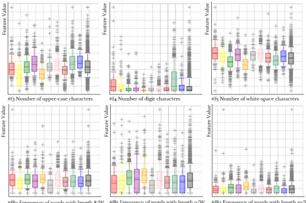
Figure 3: Examples of box-plot-based writeprint visualization scheme. Different colour (series on the diagram) stands for different candidate authors’ previous writing sampleMi.

Examples of the second visualization scheme for feature analysis are shown in Figure 3. This scheme is based on the feature value distribution and it employs the box plot to scatter the demonstrated values on specific feature for each candidate author. In this scheme, different colour stands for different candidate author, and the box plot with corresponding colouring represents how previous writing samples of this candidate author distribute on this feature.

This scheme is able to demonstrate the variation writing styles among all the candidate authors on a specific stylometric feature. Differing to the first spectrum-based scheme, all the outliers as well as the mean value and the distributional variance for each author can be easily identified. However, similar to the spectrum-based scheme, this scheme also fails to

(36)

consider the combination of feature values.

These two schemes are suitable for feature analysis and individual visualization. How-ever, for the task of authorship identification, they are impractical since they fail to combine all the features together, which assumes that the user has to inspect them one by one in each case. This assumption is unpractical since the number of features could be even more over-whelming. Also, these two types of scheme fail to answer which candidate author is more similar to the anonymous snippetω, and thus fail to visualize the solution for the authorship identification problem.

In the next chapter, we present our evidence-driven approach, which depends on dy-namic features. By combining similarity based identification approach and data mining approach, it achieves state-of-the-art identification result, at the same time its output can be visualized and interpreted. Unlike previous two types of visualization scheme, this ap-proach aims at visualizing the identification result, and it fits all the features in one diagram in an interpretable way. Based on cumulative visual effect on the diagram, the most plausi-ble author can be determined.

(37)

Chapter 4 A Visualizable Evidence-driven

Approach for Authorship Identification

In this chapter, we present our visualizable evidence-driven approach for the authorship attribution problem, addressing the issues and problems mentioned in Chapter 1. For this approach we employ the dynamic stylometric feature set, which is different to the static feature set that applied in previous chapter. In Chapter 5, we will present the experiments that compare their performance in varying identification context.

For the purpose of promoting its interpretability and explainability, our approach is designed according to the nine processes defined by the End-to-End Digital Investigation framework (EEDI) [BKW12]. Considering that every digital crime fundamentally con-sists of a source point and a destination point, the EEDI framework is a structured flow of processes to establish an evidence chain connecting these two points. EEDI is a popular framework employed by digital investigators due to its capacity of structurally organizing

(38)

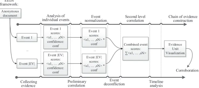
Figure 4: Overview of VEA in EEDI framework. multiple evidence sources to test the conclusion.

We design our approach by adopting the EEDI framework, based on the fact that the authorship attribution problem can also be fundamentally regarded as consisting of two points: hypothesis and conclusion. By elaborating the linguistic evidences to establish an evidentiary chain, we can connect these two points together and thus enable our approach to present the completed chain as visualized evidence. Also, the process of chain construc-tion can be easily explained by employing the EEDI framework. The briefs of procedures employed are outlined in Figure 4.

To begin with, we formally define the term authorship hypothesis (see Definition 1). Basically an authorship hypothesis is a statement that claims a candidate to be the author of a given anonymous snippetω. According to the problem defined in Sectioin 1.1, whereN candidate authors are involved, N hypotheses are thus formulated, respectively targeting on each candidate inC.

(39)

candidateC_i, a hypothesis in the authorship attribution problem is the statement that

can-didateCiauthored snippetω.

4.1 Collecting Evidence

The first phase in the original EEDI framework is Collecting Evidence [BKW12]. This phase is to detect and collect potential evidence from all available sources of information. The type of evidence may vary, for example, to identify an intrusion; evidentiary types could be logs of system access, logs of network packages, and firewall logs, etc. They required different collection and preprocessing methods. Under the EEDI framework, evi-dence of different types are grouped together and initiated into independent events, which will be passed to the next process of EEDI.

Accordingly, based on the given anonymous snippet ω, during this phase our task is to identify all the linguistic evidence. Likewise, linguistic characteristics reflected on the given snippet ω are of varying types based on their particular linguistic modalities (e.g., syntactic, lexical, and character-based, etc.), and linguistic characteristics of certain modal-ity require specific techniques for feature extraction [Sta09]. Thus, we group evidence into independent events based on their linguistic modalities, and construct them respectively.

We start this phase by defining the term evidence unit. Let F(ω) = {f1, f2, . . . , fu}

denote the universe of writing style features extracted from the anonymous snippetω. Ba-sically, an evidence unit is defined as one specific writing style feature element with its associated scoring vector (see Definition 2). Evidence unit is the minimum scoring unit

(40)

Modality Characteristics Details Examples Lexical Word Level N-gram Length:1-8 ‘It is noticed’,

‘is noticed and appreciated’ Character Character Level N-gram Length:1-8 no, not,

notic, tice, notice, a, an, and

Syntactic POS N-gram Length:1-8 PRP VBZ VBN,

CC VBN, TO DT NN Table 3: Employed lingusitic features.

and minimum visualization unit, which will be further discussed in Section 4.2.

Definition 2. (evidence unit) Evidence uniteum is formulated as set{feum, ~veum}: given

a certain linguistic featuref_eu_m,~v_eu_m ∈_RN _{is a numeric vector}_(v

1, ..., vi, ..., vN), where

N indicates the number of candidates inC, and valueviindicates the score describing the

correlation between candidateCiand the linguistic featurefeum.

The linguistic writing characteristics employed in this thesis include lexical modality, character modality, and syntactic modality. Specifically they include lexical wordn-gram, character leveln-gram, and syntactic level part-of-speechn-gram [Sta09]. Refer to Table 3 for detailed information and examples. The length of these grams varies from 1-8 because we can hardly find any gram present repetitively with length more than 8. We employ n-gram technique because previous studies [KSA11, Sav12, SVS+13] show its effectiveness in capturing the writing style. Also, they are comparatively easier to visualize and present as evidence units; more details will be discussed in Section 4.5.

To preserve the explainability of our approach, unlike previous research, we do not employ any feature selection techniques such as methods in [YP97]. That means we em-ploy the full set of grams rather than an optimal top-K subset. Previous research, such

(41)

in the authorship attribution problem, but it is hard to explain why and how this parame-terK, which indicates the size of employed features, is chosen. In the previous research, the optimal K value is learned from the presented experimental results and it is assumed that this value would work accordingly against other data. To avoid any exceptional cir-cumstance, we thus employ the full set of grams to guarantee its explainability. Even though this approach introduces high runtime complexity, it is acceptable in an investiga-tion scenario to run it only once for the purpose of collecting evidence. We believe that this trade-off between explainability and runtime complexity is reasonable.

Definition 3. (event) Given an eventevndenoted by{Tevn, Confevn, ~Vevn, EUevn},Tevn is

the type of linguistic modality with which this event is associated,EUevnis a set of evidence

units such that∀euevn

m ∈EUevn,feuevnm is of typeTevn. AlsoV~evn ∈R

N _{is a numeric vector}

of sizeN that describes to what extent this eventevnsupports each predefined hypothesis,

andConfevn ∈ [0,1]is a numeric value that indicates the confidence that this event will

arrive at its conclusion based on the present classification context.

We define event as a set of evidence units of same linguistic modality and other as-sociated properties (see Definition 3). Based on the selected linguistic feature scheme, the extraction procedure is shown in Algorithm 1. The input includes the number of candidates inC, linguistic modality typeT ype, and the anonymous snippetω. In Line 2, all features of given linguistic type are extracted from the anonymous snippetω. Based on our selected features, all the grams of given length 1 to 8 are thereby extracted and then assigned to the evidence units (see Line 5).

(42)

Algorithm 1Event Construction (EC)

Inputnumber of candidatesN, linguistic typeT ype, anonymous snippetω

Outputeventev

1: Tev ←T ype .associate this event with the given type of linguistic modality

2: f eatures ←extract all linguistic characteristics of typeTevfrom snippetω

3: form = 1to|f eatures|do

4: ~veuev

m ∈R

N_{, ~}_v euev

m ← {0} .initialize as a zero vector

5: feuev

m =f eaturesm

6: EUev ←EUev ∪ {euevm}

7: end for

8: returnev

constructions, all the events will be passed into the next process, as shown in Figure 4. In our case, three events are created: a lexical event, a character event, and a syntactic event.

4.2 Analysis of Individual Event

The second phase in EEDI process flow is to analyze each event independently. The goal in this phase is to isolate each event and access the correlation between each event and the overall investigation [BKW12]. Correspondingly, during this phase in our algorithm, we are going to independently assess each event with respect to its contribution in the overall author identification problem. For each event, two analyses are conducted:

• Scoring: to score each hypothesis (i.e., to score each candidate author) based on the given event’s feature set, and determine which hypothesis is more plausible to be the correct one.

• Consistency analysis: to evaluate the feature set of a given event regarding its ca-pability of distinguishing the writing styles among different candidates based on all

(43)

Algorithm 2Event-based Scoring (ES)

Inputeventev, writing samplesM, anonymous snippetω

Outputscoring vector:~s

1: ~s ∈_RN_,_~_s_{← {}₀_} _._{create a numeric vector of size N}

2: ~a ∈_R|EUev|_,_~a← {₀}

3: form = 1to|EUev| do

4: ~a[m] =tf(feuev

m, ω) .this vector is for anonymous snippetω

5: end for

6: fori= 1toN do

7: ~c∈_R|EUev|_,_~c_{← {}₀_} _._{this vector is for candidate author}_i

8: form = 1to|EUev|do

9: ~c[m]= tf(feuev

m, Mi)×idf(feumev) .here featurefeuevm is a gram

10: ~veuev

m[i]←~c[m]×~a[m] .store intermediate result

11: end for

12: ~s[i]=~a·~c 13: end for

14: return~s

The first analysis adopts the similarity-based approach to score each hypothesis, and it is shown in Algorithm 2. To begin with, by usingtf−idfscoring scheme and regarding all the extracted grams from an event as an unified feature vector,N + 1numeric vectors are constructed: one numeric vector~afor anonymous snippet andN candidate author numeric vectors (~cin Line 7).

Although there exist other scoring functions that may achieve higher identification ac-curacy [MFJP09] [LV09], we use the tf−idf scheme [ZM98] for its simplicity. As in Equation 2 and Equation 3, the tf score captures the normalized frequency of a given gram, and theidf score gives weight to each gram by considering its discriminant power. The constantΘis used to avoid the divide-by-zero problem, and it is typically chosen as1. We setΘas0.1, and in this way it is in a smaller order of magnitude when compared with

(44)

©

PV2 PV2’ PV1’ PV1 PV Ti Ti+1 Ti+2

Figure 5: A sample 3-gram space.

them as separate events, which could be explored in future studies.

tf(gram, Mi) =

f requency(gram, Mi)

maxGramF requency(M_i) (2)

idf(gram) = log

N

θ+|AuthorsEverU sed(gram)|

(3)

After the construction of aforementionedN+ 1numeric vectors, a final score is derived for each hypothesis (candidate) by comparing the similarity between each candidate vector ~cand the vector for anonymous snippet~a. Here we adopt thedotproductdistance to derive this score, as shown in Line 10 in Algorithm 2.

Considering a sample 3-gram space in Figure 5, P V~1, P V~ 2, and P V~ , respectively,

are the style vectors of candidate1, candidate2, and the anonymous snippet ω. In

pre-vious work such as [KSA11] wheren-gram related features are employed, thecosine dis-tance [SB88] is generally used to measure the disdis-tance between vectors. It only considers the included angles between vectors: the difference between Θ1 and Θ2 in the example.

(45)

frequency of gram usage. Regarding the direction ofP V~ as the anonymous snippet’s writ-ing style, we take the projection P V~₁0 of P V~1 on P V~ and the projection P V~20 of P V~2 on

~

P V for comparison. The projection models the amount of demonstrated evidence from a given vector and shows the strength of support of the vector in this direction. The distance function is shown in Equation 4, and for the ease of computation we multiply the norms of the anonymous vector, which is independent to the values of other vectors, and finally derive thedotproductdistance function.

similarity(P~i, ~Pω) = proj_P~_ωP~i× kP~ωk

=kP~_ik ×cos(Θ_i)× kP~_ωk

=P~i·P~ω

(4)

At the end of the first analysis (see Line 13 of Algorithm 2), each evidence unit’s scor-ing vector~v is updated with the corresponding score vi that describes the correlation

be-tween candidateiand this given linguistic feature. This updated value will be used in the visualization process elaborated in Section 4.5.

Algorithm 3 shows the second analysis. As defined in Definition 3, each event is rep-resented as a set of linguistic features. The goal of this analysis is to evaluate features of a given event with respect to their demonstrated consistency and discriminant power among the known-author writing samplesM. Such properties vary for different linguistic modalities under the given identification context (e.g., anonymous snippet length, size of known-author writing, and number of candidates, etc.). Hence, we treat each event as a

(46)

Algorithm 3Event-based Identification (EI)

Inputwriting samplesM, candidate setC, eventev, anonymous snippetω

Outputeventev

1: f olds←split(M) .splitM into 10 folds for cross-validation; each fold includes nine training groups and one validation group

2: samples← ∅; .create an empty set of samples; each sample follows at-tributes in Table 4

3: for eachf oldinf oldsdo

4: precision←tests(Tev,T rainSetf old,T estSetf old) .collect precision value

5: for eachdocinT estSetf olddo

6: ev0 ←EC(N, Tev, doc)

7: scores←ES(ev0,T rainSetf old,doc)

8: sample←generateSample(scores,doc,precision) .collect other conditions 9: samples←samples∪ {sample}

10: end for

11: end for

12: M odelev ←buildModel(samples) .build a model for this eventevusing

preci-sion as target attribute

13: V~ev←ES(ev,M,ω) .collect sample from current classification context

14: Confev ←M odelev.predict(V~ev,ω) .estimate confidence

15: returnev

stand-alone similarity-based classifier. Then a confidence value is estimated for each event in an isolated manner by building linear models. The features used to model an identifica-tion context is listed in Table 4. In this way, an event is the minimum confidence estimaidentifica-tion unit.

To proceed with this analysis, a 10-fold cross validation test is conducted by partitioning all the available writing samples fromM into ten groups of roughly equal size (Line 1 in Algorithm 3). Of these ten groups, one group is selected as a validation set, then the remaining nine groups are used to build events following Algorithm 1 and to predict the author of samples from the validation set by using Algorithm 2. The candidate with the highest score output (Line 7 in Algorithm 2) will be the predicted result. The next step is to

(47)

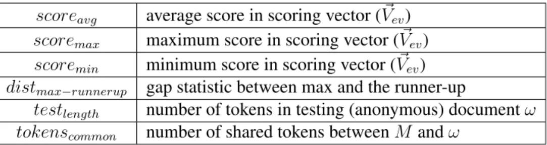
Table 4: Features for confidence estimation (identification context) scoreavg average score in scoring vector (V~ev)

score_max maximum score in scoring vector (V~_ev) scoremin minimum score in scoring vector (V~ev)

distmax−runnerup gap statistic between max and the runner-up

test_length number of tokens in testing (anonymous) documentω tokenscommon number of shared tokens betweenM andω

percentage of instances that are correctly identified) will be collected as the target attribute; other attributes shown in Table 4 will be used to construct a sample. This validation process is repeated ten times and each group is used as the validation set exactly once. Based on the collected samples, a linear regression model is built for each event (Line 12 in Algorithm 3). In Line 13, the event derives a scoring vector for given candidates based on the anony-mous snippet ω by using Algorithm 2. Based on this scoring vector, a sample is created with attributes in Table 4, and it is fed into the built model to derive the predicted precision value, which will be used as the confidence value (Line 14 in Algorithm 3).

Regarding the attributes used to model the identification context, in addition to us-ing the ‘gap statistic’ that describes the gap between max score and the runner-up in [NPG+12, KSA11, KSA06], we also include more attributes that describe the scoring dis-tribution including the maximum, the minimum, the average, and the length of testing document. Our experiment in Section 5.4 shows that these attributes are all significantly important for confidence estimation. However, we do not include the size of known-author writings, because when we conduct the 10-fold cross validation process (Line 3 to Line 12 in Algorithm 3), the intercept value in the built linear model already reflects its effect as baseline.

(48)

4.3 Event Normalization

Algorithm 4Confidence-based Normalization (CN)

Inputeventev, anonymous snippetω

Outputeventev 1: fori=1 toN do

2: V~ev[i] =V~ev[i]×Confev .normalize score for this event

3: end for

4: form = 1to|EUeu|do

5: fori= 1toN do

6: eu~ev

m[i] =eu~evm[i]×Confev .normalize the score inside each evidence unit

7: end for

8: end for

9: returnev

The event normalization process under the EEDI framework is to normalize all eviden-tiary data of the same type from different sources into the same measurement level and to further consider the possibility of combining them [BKW12]. For example, different events from different sources may have varying timing formats or different time zone settings; in order to chain them together, these formats must be normalized.

Accordingly, in our approach, after the previous process each event now has a scor-ing vector, while they have different confidence values, which means they have different performance levels on discriminating candidates. Before considering the combination of evidentiary data from these events, normalization of performance for each event must be done. Hence, we conduct our normalization step by multiplying the scoring vector with corresponding confidence value for each event (Line 2 in Algorithm 4). Also, correspond-ingly, we update the numeric vectors stored inside all evidence units of each event by multiplying the original score with the confidence value (Line 4 to 8 in Algorithm 4). After

(49)

4.4 Secondary-level Correlation

Under the EEDI framework, this process is to examine the correlation between events and to consider ways of combining the evidence into an evidentiary chain [BKW12]. In our case, accordingly, all the events from previous process are correlated and combined to derive a unidimensional score for each candidate author. The idea is to summarize the fine-grained evidence of different linguistic modalities into a single kind of evidence: the linguistic evidence.

Algorithm 5Event Combination (EC)

Inputwriting samplesM, candidate setC, set of eventEV, anonymous snippetω

Outputauthor, confidence valuep

1: f s~ ∈_RN_{, ~}_{f s}_{← {}₀_} _._{initialize final scoring vector with 0}

2: conf ∈_R|EV|_, _conf _{← {}₀_} _._{a vector of confidence values} 3: forn = 1to|EV|do

4: fori= 1toN do

5: f s[i] =~ f s[i] +~ V~evn[i]

6: end for

7: conf[n] =Confevn

8: end for

9: prediction←IndexOfMaxValue(f s)~ .determine the prediction result 10: author←C[prediction]

11: agreedConf ∈_R|EV|_, _conf _{← {}₀_} 12: forn = 1to|EV|do

13: ifevnagreespredictionthen

14: agreedConf[n] =conf[n] 15: else

16: agreedConf[n] =−1 17: end if

18: end for

19: p= max(agreedConf) .estimate the final confidence value 20: returnauthor,p

The procedure for evidence combination is shown in Algorithm 5. Since in previous process all the events have been normalized into the same identification performance level,

(50)

the final scoring vector is simply the sum of the scoring vector from each input event. In this algorithm, Line 1 to 8 combine scoring vectors from all input events, and Line 9 determines the prediction result as the candidate author that achieves the highest score.

p=maxEV evn P(predicted author| evn) =maxEV evn       

Confevn, ifevnagrees on finalpredicted author −1, otherwise

(5)

To combine multiple confidence values of different classifiers, typical approaches in-clude Product Rule, Max Rule, Min Rule, and Majority Vote Rule, etc. [KHDM98] Here we combine the Max Rule and Majority Vote Rule to derive our final estimated confidence value. As Line 12-19 in Algorithm 5 shows, the final confidence value is determined as the maximum estimated confidence value among all the events that agree on the final output candidate (also see Equation 5).

Previous research [KSA11, NPG+12] mostly combine classifiers using the ensemble method and derive the final result in a voting manner. Differently from these, we combine classifiers or, rather, events, in our case, in the scoring vector level and each scoring vector is normalized by the estimated confidence (see Equation 6). Our experiment demonstrates that this approach can achieve higher accuracy.

~ f s[k] = EV X evn ~ Vevn[k]×Confevn (6)

(51)

4.5 Chain of Evidence Construction

In this process, under the EEDI framework evidences are aligned on a timeline, and based on this timeline a coherent chain of evidence is developed [BKW12]. This chain of evi-dence is able to connect the starting point and ending point of the criminal incident. How-ever, in our solution, temporal priority among all linguistic evidence is nonexistent. Based on the employed dot-point distance, the cumulative effect of evidences is instead estab-lished from hypotheses to conclusion.

~ f s[k] = EV X evn EUevn X euevnm ~v_euevn m [k] (7)

At this point, based on the input events the cumulative effect to derive the final uni-dimensional score for each hypothesis can be expressed as Equation 7 by employing the intermediate results stored in evidence units according to Algorithm 2 and Algorithm 4.

~

f s[k]refers to the final score for candidatek in Algorithm 5, which is also the same vari-able in Equation 6 but is calculated using different intermediate results.

The task of this process is to visualize all the evidence units with respect to their dis-tance to each hypothesis. The visually cumulative effect of all evidence units should be able to reflect the difference between candidate scores f s[k]. Formally, a visual measurement~ functionvf should have the following property:

Property 4.5.1. (proportionally visualizable) Given a set of hypotheses H, we say they

are proportionally visualizable over a visual effect functionvf if they satisfy: ∀Hk ∈ H

(52)

To begin with, hypotheses are visualized. As defined in Definition 1, the hypothesis is the statement that an anonymous snippet ω is authored by one specific author. Given N candidates inC, we thus haveN hypotheses, and each hypothesis is represented by the raw tokens extracted from the anonymous snippet ω with the corresponding statement about one specific candidate.

N_VUZNKYOY IGTJOJGZK>OYZNKG[ZNUX N_VUZNKYOY IGTJOJGZK?OYZNKG[ZNUX

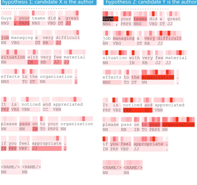
Figure 6: Evidentiary chain visualization: hypothesis representations and the visualized evidence units.

(53)

represented by the hypothetical statement on the title along with the following evidence ex-tracted from anonymous snippetω: the first row represents character level tokens, the sec-ond row represents word level tokens, and the third row represents Part-Of-Speech tokens. To make the representation simpler and clearer, in the first row we display the character tokens with a transparent font colour so that each character token can be easily matched to the lexical token beneath.

After presenting the visualizations of hypotheses we are going to visualize all evident units (defined in Definition 2) by colouring each evidence unit’s tokens in the above repre-sentations of hypotheses. The colour is determined by how affiliated an evidence unit is to the given hypothesis. An evidence unit hereby is our smallest visualization unit.

To colour the tokens the HSL colour scheme is employed because it is more intuitive than the RGB colour scheme [ÇLB12]. The HSL scheme encodes colour by using three parameters: Hue, Saturation, and Lightness. Hue represents the selected tint ranging from 0 to 360, and in most cases it is used as a qualitative representation in data visualization: the difference in kinds reflected in the difference of tint. Saturation controls its colourfulness (from 0 to 100), and Lightness measures how much light should be reflected from this colour, ranging from 0 (appears as black) to 100 (appears as white); 50 isnormal[ÇLB12]. Lightness is visually suitable as a quantitative/sequential data representation. Dark equals moreis a standard cartographic convention [HB03] and the difference of lightness can still be perceived by people with red-green colour vision impairments [HB03]. Thus we adopt the lightness value representing the scores of evidence units.

Based on our observation, given an evidence unit euevn

(54)

in most cases the range of this vectorrange(~v_euevn

m )is only a small fraction of the overall

score range. Simply picking up the lightness value of the given evidence unit euevn m , for

hypothesis k based on its score ~v_euevn

m [k], will naturally lead to the imperceptible visual

discrimination among hypotheses. Hence, instead of visualizing the original scores, we visualizedif(euevn

m , k)in Equation 8, which represents how the original score differs from

the minimum score in that scoring vector. The constantα >1is used to magnify the range, avoiding assigning a blank background on euevn

m for hypotheses k when~veuevnm [k] equals

min(~v_euevn

m ), because if~veuevnm [k]6= 0, eu evn

m still contributes to the overlapping effect in the

colouring process, which will be discussed later. To calculate the valuedif(euevn

m , k)for each hypothesiskon each evidence uniteuevmn,

the global rangemaxRof the scaled difference is first calculated by using first three equa-tions in Equation 8. The range of the scaled difference in scoring vectors is calculated for each event and then all ranges are combined to reach maxR (globally maximum scaled difference in all scoring vectors).

range0(eum) = max(~veum)×α−min(~veum)

maxRevn =max({eu evn

m ∈EUevn |range

0_(euevn m )})

maxR=max({evn∈EV |maxRevn})

dif(euevn m , k) = ~ v_euevn m [k]×α−min(~veum) maxR (8)

(55)

same token in the hypothesis representation. Accordingly, each evidence unit is coloured in an overlapping manner. LHk tokenn(eu evn m ) =        LHk

tokenn−η×dif(eu evn

m , k), ifeuevmn stem fromtokenn

LHk

tokenn otherwise

(9)

Given a visual representation of hypothesisHk, we start by initializing all tokens’

back-grounds with a maximum lightness value (i.e., the background colour reflects 100% light and appears to be blank), and then we enumerate tokens in the hypotheses representation to apply Equation 9. Given atokenninHk, for each previously extracted evidence uniteuevmn,

iffeuevn

m stems fromtokennthen the token’s lightness value degrades by the multiplication

of degradation factorηand its normalized variant scoredif(euevn

m , k). Degradation factor

η∈(0,100]controls the contrast between hypotheses and can be designated by the user or empirically as100.0/M axM atch, whereM axM atchindicates the maximum number of evidence units that can stem from the same token. euevn

m stems fromtokennmeans that the

evidence unitseuevn

m partially or completely originates from thetokenn. For example,

evi-dence unit “your organization” can stem from token “your” in phase “to your organization” but not from the token “your” in phase “your teams”.

Since this “stem” mapping between tokens and evidence units is identical for all the hypotheses, given the same evidence unit the lightness value of a token is inversely pro-portional to the score dif(euevn

m , k) of the hypothesis. In this way, it is also inversely

proportional to the original score~v_euevn

(56)

LHk tokenn(eu evn m )∝dif(euevmn, k)−1 ∝(~v_euevn m [k]−min(~veuevnm )) −1 ∝~v_euevn m [k] (10)

Our selected visual function vfVEA(Hk) for hypothesisk is the global darkness of its

visual representation, denoted byGD(Hk), which is inversely proportional to the global

lightness GL(Hk)function. We assume that the global lightness value is contributed by

the cumulative lightness of all tokens on the representation. This assumption is reasonable when the anonymous snippet is short.GD(Hk)is formulated in Equation 11.

vfVEA(Hk) =GD(Hk) ∝GL(Hk)−1

(11)

It can be shown that this visual function satisfies Property 4.5.1 as follows: First, the global lightness function GL(Hk)for hypothesisk is formulated as the cumulative

light-ness of all tokens (see Step 1 in Equation 12). By combining Equation 10, the GL(Hk)

function is inversely proportional to the final score of hypothesisk (see Step 2-5 in Equa-tion 12).

(57)

GL(H_k) = tokens(Hk) X tokenn EV X evn EUevn X euevnm LHk tokenn(eu evn m ) ∝ tokens(Hk) X tokenn EV X evn EUevn X euevnm dif(euevn m , k) −1 ∝ tokens(Hk) X tokenn EV X evn EUevn X euevnm ~veuevnm [k] −1 ∝ EV X evn EUevn X euevnm ~v_euevn m [k] −1 ∝f s[k]~ −1 (12)

In this way, by combining Equation 11, the visual function GD(H_k) is proportional to the final score of hypothesis k (see Equation 13). Thus, our selected presentation of hypothesis and evidence unit satisfies Property 4.5.1 over visual functionGD(Hk), which

indicates that the darker the hypothesis representation’s holistic colour is, the higher final score this hypothesis possesses.

vfVEA(Hk) =GD(Hk) ∝GL(Hk)−1 ∝f s[k]~

(13)

After all the aforementioned colouring is done, one can conclude that the hypothesis with the most holistically darkest colouring representation is the most plausible one. As the example in Figure 6 demonstrates, representation of hypothesis 2is more holistically

Authorship Identification and Writeprint Visualization

AUTHORSHIP IDENTIFICATION AND WRITEPRINT

VISUALIZATION

C

ONCORDIA

UNIVERSITY

School of Graduate Studies

Abstract

Authorship Identification and Writeprint Visualization

Acknowledgments

Contents

List of Figures

List of Tables

Chapter 1

Introduction

1.1

The problem

1.2

Challenges and Contributions

1.3

Thesis Organization

Chapter 2

Related Works

2.1

Stylometric Features

2.2

Attribution Techniques

2.3

Ensemble Method

2.4

Adversary Stylometry

2.5

Attribution Result and Result Visualization

Chapter 3

Analysis of Static Stylometry

3.1

Static Stylometry and Data Representation

3.2

Similarity-based Approach and Distance Functions

3.3

Analysis through Visualization

Chapter 4

A Visualizable Evidence-driven

Approach for Authorship Identification

4.1

Collecting Evidence

4.2

Analysis of Individual Event

©

©

4.3

Event Normalization

4.4

Secondary-level Correlation

4.5

Chain of Evidence Construction