Genomic Meta-Analysis Combining Microarray Studies with Confounding Clinical Variables: Application to Depression Analysis

GENOMIC META-ANALYSIS COMBINING

MICROARRAY STUDIES WITH CONFOUNDING

CLINICAL VARIABLES: APPLICATION TO

DEPRESSION ANALYSIS

by

Xingbin Wang

MS, Shanghai Jiaotong University CHINA, 2005

Submitted to the Graduate Faculty of

the Graduate School of Public Health in partial fulfillment

of the requirements for the degree of

Doctor of Philosophy

University of Pittsburgh

2011

UNIVERSITY OF PITTSBURGH GRADUATE SCHOOL OF PUBLIC HEALTH

This dissertation was presented by

Xingbin Wang

It was defended on August 15 2011 and approved by

George C. Tseng, ScD, Associate Professor, Department of Biostatistics Graduate School of Public Health, University of Pittsburgh

Etienne Sibille, Ph.D, Associate Professor, Department of Psychiatry School of Medicine, University of Pittsburgh

Allan Sampson, Ph.D, Professor, Department of Statistics School of Arts & Sciences, University of Pittsburgh

Yan Lin, Ph.D, Assistant Professor, Department of Biostatistics Graduate School of Public Health, University of Pittsburgh

Dissertation Director: George C. Tseng, ScD, Associate Professor, Department of Biostatistics

GENOMIC META-ANALYSIS COMBINING MICROARRAY STUDIES WITH CONFOUNDING CLINICAL VARIABLES: APPLICATION TO

DEPRESSION ANALYSIS Xingbin Wang, PhD University of Pittsburgh, 2011

Major depressive disorder (MDD) is a heterogeneous psychiatric illness with mostly un-characterized pathology and is the fourth most common cause of disability according to the World Health Organization (WHO) and has a significant impact on public health in the United States. To understand the genetics of MDD, we aim to develop effective meta-analysis approaches to provide high-quality characterization of MDD related biomarkers and path-ways with proper clinical variable adjustment. First, genomic meta-analysis in MDD faces multiple unique difficulties, such as weak expression signal of MDD, substantial clinical het-erogeneity and small sample size. Given these obstacles, it is hard to identify consistent and robust biomarkers in an individual study. To achieve a more accurate and robust detection of differentially expressed (DE) genes and pathways associated with MDD, we proposed a statistical framework of meta-analysis for adjusting confounding variables (MetaACV). The result showed that more MDD related biomarkers and pathways were detected that greatly enhanced understanding of MDD neurobiology. Secondly, Meta-analysis has become popu-lar in the biomedical research because it generally can increase statistical power and provide validated conclusions. However, its result is often biased due to the heterogeneity. Meta-regression has been a useful tool for exploring the source of heterogeneity among studies in a meta-analysis. In this dissertation, we will explore the use of meta-regression in mi-croarray meta-analysis. To account for heterogeneities introduced by study-specific features such as sex, brain region and array platform in the meta-analysis of major depressive disorder

(MDD) microarray studies, we extended the random effects model (REM) for genomic meta-regression, combining eight MDD microarray studies. The result shows increased statistical power to detect gender-dependent and brain-region-dependent biomarkers that traditional meta-analysis methods cannot detect. The identified gender-dependent markers have pro-vided new biological insights as to why females are more susceptible to MDD and the result may lead to novel therapeutic targets. Finally, we present an open-source R package called Meta-analysis for Differential Expression analysis (MetaDE) which provides 12 commonly used methods of meta-analysis. It is a friendly used software such that biologists implement meta-analysis in their research.

TABLE OF CONTENTS

1.0 INTRODUCTION . . . 1

1.1 MAJOR DEPRESSIVE DISORDER . . . 2

1.2 DATA DESCRIPTION AND PROBLEMS ENCOUNTERED IN GENE EXPRESSION ANALYSIS . . . 4

1.3 EXISTING METHODS FOR DE GENE DETECTION IN SINGLE STUDY 5 1.3.1 T-TEST. . . 6

1.3.2 Paired T-TEST. . . 6

1.3.3 MODERATED T-TEST. . . 7

1.3.4 LINEAR REGRESSION MODEL . . . 7

1.4 EXISTING MICROARRAY META-ANALYSIS METHODS . . . 8

1.4.1 METHODS COMBINING P-VALUES . . . 9

1.4.1.1 Fisher’s method(Fisher) . . . 9

1.4.1.2 Tippett’s method(minP) . . . 9

1.4.1.3 Wilkinson’s Method(maxP). . . 10

1.4.1.4 Generalized ordered statistics(rOp) . . . 10

1.4.1.5 Stouffer’s Method(Stouff) . . . 10

1.4.1.6 Adaptively weighted Fisher’s Method(AW) . . . 11

1.4.2 METHODS COMBINING EFFECT SIZES . . . 11

1.4.2.1 Fixed Effects model(FEM) . . . 14

1.4.2.2 Random Effects model (REM) . . . 15

1.4.2.3 Fixed effects model versus Random effects model . . . 15

1.5.1 Fisher’s Exact Test. . . 17

1.5.2 Kolmogorov-Smirnov (KS) Test . . . 18

2.0 A SYSTEMATIC STATISTICAL APPROACH TO INTEGRATE WEAK-SIGNAL MICROARRAY STUDIES ADJUSTED FOR CONFOUND-ING VARIABLES WITH APPLICATION TO MAJOR DEPRESSIVE DISORDER . . . 20

2.1 MOTIVATIONS . . . 20

2.2 MATERIALS . . . 22

2.3 METHODS . . . 24

2.3.1 Single study analysis for DE gene detection . . . 24

2.3.2 Meta-analysis for DE gene detection . . . 28

2.3.3 Pathway analysis . . . 28

2.3.4 Post hoc analysis on the confounding variables after meta-analysis . 29 2.3.5 Evaluation and simulation . . . 30

2.4 RESULTS AND DISCUSSION . . . 31

2.4.1 Recommended statistical framework . . . 31

2.4.2 Comparison of various methods in single study analysis . . . 32

2.4.3 Comparing three meta-analysis methods in combining all five studies 34 2.4.4 Distribution of covariate inclusion in the models of detected DE genes 40 2.4.5 Simulation results . . . 42

2.5 Discussion . . . 42

3.0 META-REGRESSION MODELS TO DETECT BIOMARKERS CON-FOUNDED BY STUDY-LEVEL COVARIATES IN MAJOR DEPRES-SIVE DISORDER MICROARRAY DATA. . . 46

3.1 INTRODUCTION . . . 46

3.2 METHODS . . . 48

3.2.1 Description of motivating MDD data . . . 48

3.2.2 Data preprocessing, gene matching and gene filtering . . . 49

3.2.3 Single study analysis incorporation sample-level variables . . . 50

3.2.5 Post hoc analysis on study-level variables after meta-regression . . . 54

3.2.6 Evaluation . . . 55

3.3 RESULTS . . . 57

3.3.1 Fixed effect model and Random effect model . . . 57

3.3.2 comparing individual analysis and meta-analysis . . . 57

3.3.3 Comparing REM and MetaRG . . . 58

3.3.4 Frequencies of study-level covariates confounded with disease effect . 60 3.3.5 Result of Komogorv-Smirnow test . . . 62

3.4 DISCUSSION AND CONCLUSION. . . 63

4.0 METADE: A R PACKAGE TO PERFORM META-ANALYSIS FOR DIFFERENTIAL EXPRESSION ANALYSIS . . . 65

4.1 INTRODUCTION . . . 65

4.1.1 Meta-analysis methods with one-sided correction . . . 67

4.1.1.1 Notations. . . 67

4.1.1.2 Pearson’s method(Fisher OC) . . . 68

4.1.1.3 minP method with one-sided correction(min OC) . . . 69

4.1.1.4 maxP method with one-sided correction (maxP OC) . . . 70

4.1.1.5 roP method with one-sided correction(roP OC) . . . 70

4.2 IMPLEMENTATION. . . 71

4.2.1 Data pre-processing . . . 73

4.2.2 Perform individual analysis . . . 74

4.2.3 Perform meta-analysis . . . 75

4.2.4 Draw plots . . . 77

4.2.5 EXAMPLE . . . 77

4.3 DISCUSSION AND CONCLUSION. . . 81

5.0 CONCLUSIONS AND FUTURE WORKS . . . 83

5.0.1 CONCLUSIONS . . . 83

5.0.2 FUTURE WORKS. . . 84

APPENDIX A. ALGORITHM OF PERMUTATION ANALYSIS . . . 87

APPENDIX C. ALGORITHM OF META-REGRESSION ANALYSIS . . 90

APPENDIX D. THE PROOF OF ONE-SIDED CORRECTION METHODS 91

APPENDIX E. TABLE OF SIMULATIONS . . . 99 APPENDIX F. TEN MDD RELATED GENES . . . 101 BIBLIOGRAPHY . . . 103

LIST OF TABLES

1.1 Data description of eight MDD microarray studies . . . 4 1.2 2×2 Contingency Table for Pathway Enrichment Analysis. . . 18 2.1 Data description of five MDD microarray studies . . . 22 2.2 Pearson correlation between covariates in three MDD cohorts (collinearity evaluation) 23 2.3 The number of significant interaction terms between disease state and covariates in

FEM model and RIM. . . 27 2.4 Results of individual study analyses and meta-analysis combining p-values calculated

from RIM minP . . . 37 2.5 Frequency of covariates appearing in RIM minP models among 664 DE genes

de-tected by maxP method under p-value threshold 0.005. Rank is shown in parentheses and rank average of each covariate is calculated to indicate relative degree of fre-quency that a covariate impacts gene expressions and confounds with disease effect 41 2.6 Evaluation of t-test, FEM minP, FEM BIC and FEM ALL methods by

simula-tions.The Average of Type I errors, average of statistical powers, and average number of detected DE genes by each method are shown. . . 43 3.1 Results of individual study analyses and meta-analysis . . . 59

LIST OF FIGURES

2.1 Simulated null distributions of disease effect p-value in the best model (left: RIM minP; right: RIM BIC) from permutation analysis in the five MDD stud-ies. The result shows bias (deviation from uniform distribution) caused by variable selection. . . 26 2.2 Three correlation structures of interest among disease variables X, gene

ex-pression variable Y and covariates Z that are used in the simulation. Scenario I: gene expression depends on both disease state and covariates. Scenario II: gene expression depends only on disease state. Scenario III: gene expression depends on disease state directly and depends on covariates indirectly through disease state. . . 31 2.3 Three correlation structures of interest among disease variables X, gene

ex-pression variable Y and covariates Z that are used in the simulation. Scenario I: gene expression depends on both disease state and covariates. Scenario II: gene expression depends only on disease state. Scenario III: gene expression depends on disease state directly and depends on covariates indirectly through disease state. . . 33 2.4 Comparison of RIM minP, RIM BIC and RIM ALL in individual study

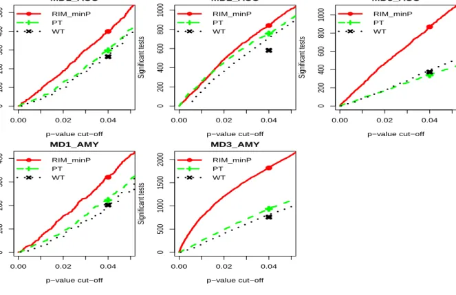
anal-yses. The result showed that RIM minP detected the largest number of DE genes among the three methods. . . 34 2.5 Comparison of RIM minP, paired t-test (PT) and Wilcoxon signed-rank test

(WT) in individual study analyses. The result showed that RIM minP detected the largest number of DE genes among the three methods.. . . 35

2.6 Comparison of RIM minP and FEM minP in individual study analyses. The result showed that RIM minP usually detected more DE genes. . . 36 2.7 Venn diagram of DE gene lists obtained from Fisher, maxP and IVW under

0.005 p-value threshold. . . 38 2.8 Heatmap of minus log10-transformed p-values obtained from all five studies

and meta-analysis for detecting DE genes. Red indicates small p-values and green indicates large p-values. (A) DE genes detected by Fisher’s method but not by maxP method; (B) DE genes detected by maxP but not by Fisher’s method; (C) DE genes detected by both Fisher and maxP method. . . 39 3.1 Gene by gene testing for the homogeneity of study effects. Overall test results

are shown by the histogram of the observed Q values and the plot of the observed versus expected Q quantiles for the 8 MDD studies . . . 58 3.2 The DE number plot of both meta-analysis and individual analyses under

various FDR thresholds.. . . 60 3.3 (a) the venn diagram of DE gene lists detected by REM and MetaRG at FDR

1%. (b) the density plot of q-values calculated from MetaRG for three cate-gorical sets of DE genes.(c) The density plot of q-values calculated from REM for three categorical sets of DE genes . . . 61 3.4 (a) the forest plot of gene SST. (b) the forest plot of gene ELP3. . . 62 3.5 The number of genes detected from both meta-analysis and individual analyses

among 156 MDD-related genes under various FDR thresholds. . . 63 4.1 Summary of 12 microarray meta-analysis methods included. . . 72 4.2 The heatmap of DE genes detected by maxP method under p-value threshold

0.001 based result of paired t-test in individual analysis. . . 78 4.3 (A)The DE number plot of paired t-test.(B) The DE number plot of MetaACV. 81 5.1 The flow chart of a hierarchical meta-analysis. . . 85 5.2 The diagram of hierarchical meta-analysis. . . 86 E1 Simulation scheme of three correlation structures in Scenario I, II and III. (X:

F1 The direction of covariates effect in RIM minP models for 10 MDD related genes from literature. . . 102

PREFACE

This thesis is based upon studies conducted during August 2006 to August 2011 at the Department of Biostatistics, Graduate School of Public Health, University of Pittsburgh. Many inspiring people have been involved in the work leading to my PhD thesis. I will like to acknowledge everyone for their contributions to the studies conducted during my time as a PhD student.

First and foremost, I would like to express my sincere gratitude to my supervisor, Dr. Chien-Cheng Tseng (George), for his excellent and inspiring supervision of my work. He has been a great mentor and a great friend, without his instruction and unique support, this thesis would never have become a reality. Further I would like to thank my co-supervisor, Dr. Etienne Sibille, for his great and invaluable co-operation and help.

I thank all the members of my committee, Dr. Allan Sampson, Dr. Yan Lin for the many discussions and their critical comments on my thesis. I also thank all the members of my learning group, Jia Li, Zhibao Mi, Kui Shen, Shuya Lu, Sunghee OH, Chi Song(Chuck), Dongwan Kang and Lun-Ching Chang, for creating a nice studying and working environment in our office and their willingly participation in many interesting discussions.

Finally, I wish to express my greatest thanks to my family, my wife, Xinmei Zhu, who has been supporting me in many ways during the past years. She has been doing biomedical research for many years. It was her who introduced biostatistics to me several years ago, in that meanwhile, I was a mathematician. She let me know how important the statistical analysis is for medical research. Thereafter, I started to like biostatistics and finally chose the PhD program of biostatistics after I got my Master degree of Science. I have truly been fortunate, and I do appreciate her support during PhD study. I also thank my daughters, Ellin Wang and Raelyn Wang, who bring lots of joy to me.

1.0 INTRODUCTION

Major depressive disorder (MDD) is a heterogeneous psychiatric illness with mostly un-characterized pathology, contributs to death by suicide, and is the fourth most common cause of disability according to the World Health Organization (WHO). To understand the genetics of MDD, gene expression analysis is a effective approach to identify the biomarkers associated with MDD. Differentially expressed (DE) gene detection is one of the most com-mon analyses in microarray data, which are generally comprised of three components: (1) the gene expression data; (2) the outcome variable, such as disease status; and (3) patient-specific covariates, including treatment history and additional clinical and demographic information. The primary aim of many gene expression studies is to identify the DE genes by character-izing the relationship between the first two of these components, the gene expression and the disease outcome. Thus, in the literature, most psychiatric disease-related microarray studies of similar design did not carefully consider how these factors (the third component) influence the relationship between the gene expression and the disease status. Usually they either ignored the clinical variables or applied simple linear regression to include all variables in the model. Our results clearly show the limits to those two approaches. To our knowledge, this is the first study that systematically considers the critical elements in the data structure in order to obtain more accurate DE gene and pathway detection. In addition, due to the very weak expression signal of MDD, a substantial clinical heterogeneity and small sample size, it is hard to identify consistent and robust biomarkers in an individual study. In this dissertation, we aim to develop effective meta-analysis approaches to fill this gap and provide high-quality characterization of MDD related biomarkers and pathways with proper clinical variable adjustment.

This dissertation is organized as follows: in Chapter 1, the concept of MDD is first described in section 1.1; then, the statistics used in individual analysis, meta-analysis and pathway analysis methods are reviewed in sections1.3,1.4and1.5, respectively. In chapter2, we describe a statistical approach for meta-analysis to tackle weak signal expression profiles that have small sample size, case-control paired design and confounding covariates in each study. In Chapter3, a meta-regression model with variable selection is described. In Chapter 4, the implementation and usage of the MetaDE package are described. Conclusions and future works are provided in Chapter 5.

1.1 MAJOR DEPRESSIVE DISORDER

Major depressive disorder (MDD) is a mental disorder characterized by an all-encompassing low mood accompanied by low self-esteem, and by loss of interest or pleasure in normally enjoyable activities. MDD is a disabling condition which adversely affects a person’s family, work or school life, sleeping and eating habits, and general health[65]. It involves a minimum two-week continuous period of at least five of the following symptoms: lowered mood for the majority of the day, diminished pleasure in daily activities, weight loss or gain, sleep disturbance, agitation or lethargy, fatigue, feelings of worthlessness or helplessness, impaired thought or memory, and recurring thoughts of self-harm or death (DSM-IV 2000). Depression is a common human psychiatric disorder and the leading cause of disability in North America, afflicting an estimated 18% of the population with an approximate lifetime incidence of 12% in men and 20% in women [55]. Around 3.4% of people with major depression commit suicide, and up to 60% of people who committed suicide had depression or another mood disorder. The symptoms of depression are the greatest contributor to the global burden of disease [46] as calculated by total days lived with the disorder. It remains the fourth leading cause of worldwide disability, after accounting for higher mortality in other diseases. This ranking is expected to rise to second place by the year 2020, as current effective treatment for other diseases become more globally accessible.

Risk factors for depression: Major risk factors for depression include the sex of an in-dividual, previous history of the illness, genetic predisposition/family history, and chronic or acute stress [30]. Some combination of these can prompt a depressive episode, but the requisite combination varies by individual. The threshold for depression is sensitive to social support, religiosity, age, and life stressors [14, 56, 57]. These environmental factors interact with the genetics of depression estimated at 33% heritance [30]. This is a lower heritability than bipolar disorder, or schizophrenia, which adds to the difficulty in teasing apart con-tributory factors. Depression itself is a risk factor for the disorder, as untreated depression is likely to reoccur [70]. This is particularly problematic as a significant percentage of pa-tients (varying from placebo levels of 30%, up to 40% depending on the study) never meet the criteria for complete remission and will commonly endure increasingly lengthy bouts of depression [36, 58].

Complexity obscure the neuropathology of depression: Depression’s continued toll on society is a function of multiple genetic and environmental susceptibilities that recruits a di-verse cadre of further genetic factors to sustain the condition [6]. To date, most experiments have examined single aspects of the disease, but the complex causal factors in depression make it resistant to highly specific approaches. One immediate question is: Why not cre-ate sub-divisions of depression that have more homogeneous symptom groups that will be amenable to a pathology classification? However, clinical evidence does not strongly support this approach. In patients with repeated depressive episodes there is no correspondence of symptoms across episodes, preventing definitive clinical subdivisions that might have more consistent pathophysiology[74]. There is some evidence to suggest that classes of antidepres-sants have distinct response rates in different DSM-IV classifications of depression (atypical, psychotic, bipolar etc) [4]. However, a meta-analysis of over 100 antidepressant drugs trials found no difference in response rates as an interaction of drug class and putative subtype[17].

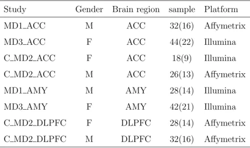
Table 1.1: Data description of eight MDD microarray studies

Study Gender Brain region sample Platform MD1 ACC M ACC 32(16) Affymetrix MD3 ACC F ACC 44(22) Illumina C MD2 ACC F ACC 18(9) Illumina C MD2 ACC M ACC 26(13) Affymetrix MD1 AMY M AMY 28(14) Illumina MD3 AMY F AMY 42(21) Illumina C MD2 DLPFC F DLPFC 28(14) Affymetrix C MD2 DLPFC M DLPFC 32(16) Affymetrix

1.2 DATA DESCRIPTION AND PROBLEMS ENCOUNTERED IN GENE

EXPRESSION ANALYSIS

Data description In this dissertation, we will focus on 8 human studies listed in Table 1.1 obtained from Dr. Sibille’s lab for meta-analysis. In most of the patient cohorts, MDD patients are matched to control patients by their demographics such as age, sex and race. MDD related clinical variables of the patients are available for most studies, including alcohol consumption (AH), history of taking anti-depressant drugs (AD), death by suicide (SC), pH level of brain tissues (pH), disease recurrence (RC) and postmortem interval (PMI). Each study has three study-level features that may need adjustment in the analysis: sex, brain region, and array platform.

Problems encountered in gene expression analysis: Detecting candidate markers in tran-scriptomic studies is often difficult in MDD studies: First, as described in section1.1, MDD is thought to be a complex and heterogeneous disease, associated with multiple genetic, genomic, post-translational, and environmental factors. Furthermore, patients might have varying disease severity, with some having psychotic features as well as exposure to a variety of medications and dosage levels to control their illness. Secondly, the genetic disease effects

are potentially confounded by many covariates, which include (1) demographical variables such as age, sex and race; (2) clinical variables such as anti-depressant drug usage, death by suicide and alcohol dependence; (3) technical variables inherent in the use of post-mortem brain samples, such as the pH level of brain tissues, brain region and post-mortem interval (PMI). If the statistical models employed to identify differentially expressed genes fail to incorporate these sources of heterogeneity, not only can this reduce the statistical power, but also it will introduce sources of spurious signals to the gene detection. Finally, sample sizes for these studies are generally small (between 9-22 pairs of MDDs and controls) due to the limited availability of suitable brain specimens and the significant costs associated with their collection. These three features in MDD studies severely hamper accurate biomarker detec-tion. In section1.3, we listed several statistical methods often used in the literature for DE gene detection in individual analysis, such as paired or unpaired t-test or the simple linear regression model. The former approach undoubtedly ignored the effects from confounding covariates; the latter approach was not efficient or not even applicable when the number of covariates is large and the number of samples in each study is small. These methods have been shown to have low statistical power in each MDD study with weak signal expression profiles, small sample size, case-control paired design and confounding covariates.

1.3 EXISTING METHODS FOR DE GENE DETECTION IN SINGLE STUDY

Gene-expression microarrays hold tremendous promise for revealing the patterns of coor-dinately regulated genes. Because of the large volume and intrinsic variation of the data obtained in each microarray experiment, statistical methods has been used as a way to sys-tematically extract biological information and to assess the associated uncertainty. SAM and LIMMA are popular methods for microarray. Methods we covered here are more naive versions.

1.3.1 T-TEST

The t test perhaps is the most popular method for detecting differentially expressed genes due to its simplicity and availability. The t statistic is defined as

Tg = ¯ YD −Y¯C S √ 1 nD + 1 nC , (1.1)

where ¯YD and ¯YC are the mean values of disease (MDD) and control groups; nD and nC are the number of replicates in disease and control groups. S is the pooled standard deviation, which is estimated by S =

√

(nD−1)S2

D+(nC−1)SC2

nD+nC−2 . Under normal assumption, Tg follows a central student’s t distribution with degree of freedom nC +nC −2 under null hypothesis if we assume that MDD and control group have the same variance and the experiment was not pair-designed.

1.3.2 Paired T-TEST

The matched groups design is another popular form in medicine research in which subjects from disease and control groups are matched on some demographic variables such as age, gender and race. In this situation, paired t-test is the conventionally used test, which is defined as, Tg = ¯ YD −Y¯C S √ 1 n , (1.2)

where S is the standard deviation of differences of each pair, which is estimated by S =

√∑n

i=1[(YDi−YCi)−( ¯YD−Y¯C)]2

(n−1) . Tg follows Student’s t distribution with degree of freedom of n−

1 under assumptions that the paired differences are independent and identically normally distributed. In general, paired test has more power than unpaired test whenever the within-pairs covariance is positive. Note that an alternative to the paired Student’s t-test when the population can not be assumed to be normally distributed is the Wilcoxon singed-rank test[102].

1.3.3 MODERATED T-TEST

The gene-specific t test is not affected by heterogeneity in variance across genes because it only uses information from one gene at a time. It may, however, have low power because the sample size is small. In addition, the variances estimated from each gene are not stable: for example, if the estimated variance for one gene is small, by chance, the Tg value can be large even when the corresponding mean difference is small. To account for gene-specific fluctuations, a moderated t statistics [27, 99] is defined as below,

Tg = ¯

YD −Y¯C

sg+s0

, (1.3)

where ¯YD and ¯YC are the mean values of expression for gene g in disease and control groups, respectively; sg is the standard deviation of repeated expression measurements:sg =

√ [(nD−1)S2 D+(nC−1)SC2][ 1 nD+ 1 nC]

nD+nC−2 ; s0 is a positive constant to minimize the variability among

sg(1 ≤g ≤ G). In SAM, a regression procedure was used to select the optimal value of s0.

For simplicity,s0 was often selected as the median ofsg. With this modification, genes with small mean differences will not be selected as significant, and this removes the problem of stability mentioned above.

1.3.4 LINEAR REGRESSION MODEL

A simple linear regression model[67, 76] has been commonly used to detect DE genes to account for additional variability resulting from many confounding variables. (e.g., in MDD studies, Age, pH, PMI and RIN). The model is described as below:

Ygi=µg+βg0X0i+ L

∑

l=1

βglXli+ϵgi, (1.4)

In the model, Ygi was the gene expression value of gene g(≤ g ≤ G) and sample i . X0i was the disease label that took value one if the sample was disease and zero if sample was a control. Xli represented values for potential confounding covariate l (1≤l≤L); 0-1 binary for categorical variables of two levels and numerical for continuous variables). Finally, ϵgi were independent random noises that followed a normal distribution with mean zero and

variance σ2

g. Under this model, βg0 was the disease effect of gene g and was the parameter

of major interest. To obtain a disease-associated biomarker candidate list in a single study analysis, likelihood ratio test (LRT) or wald test was used to assess the p-values of testing

H0 :βg0 = 0 (vs HA:βg0 ̸= 0).

1.4 EXISTING MICROARRAY META-ANALYSIS METHODS

Many high-throughput genomic technologies have advanced dramatically in the past decade. Microarray experiment is one example that evolved into relative maturity with general con-sensus experimental protocol and data analysis strategy. Its extensive application in the biomedical field has led to an explosion of gene expression profiling studies publicly avail-able. The noisy nature and small sample size in each dataset, however, often result in inconsistent biological conclusions. Consequently, meta-analysis methods for combining mi-croarray studies have been widely applied to increase statistical power and provide validated conclusions. Four major categories of statistical methods have been used to combine microar-ray studies in differentially expressed (DE) gene detection: combining p-values, combining effect sizes, combining ranks and directly merge after normalization. In this dissertation, we mainly focused on the first two categories, one is to combine statistical significance (p-value)[52, 79, 80] from each individual study, and the other is to combine the effect sizes [15, 66]from each individual study. In general, among these microarray meta-analysis meth-ods used in the literature, most methmeth-ods have their pros and cons depending on the data structure and biological goal [47, 78]. Briefly, methods based on combining p-values are free of distribution assumptions and more powerful when the studies combined are heterogeneous, but do not support inferences about magnitudes and directions. On the other hand, meth-ods based on combining effect sizes provide information about magnitudes and directions (e.g. down-regulated or up-regulated), but are more stringent on assumptions. In section 1.4.1, we described several representative methodologies for the first category. The represen-tative methodologies for the second category were described in section 1.4.2. In these two sections, we consider K independent experiments have been performed to detect a certain

effect, θgk is the parameter that characterizes the condition (e.g. disease) effect in study

k, k = 1,2,· · · , K for gene g,(1 ≤ g ≤ G). The kth experiment is concerned to test the hypothesis H0gk : θgk = 0 against an alternative H1gk : θgk ̸= 0, and the p-value associated with the above test is denoted aspgk.

1.4.1 METHODS COMBINING P-VALUES

1.4.1.1 Fisher’s method(Fisher) Fisher’s method (Fisher)[31, 32]is perhaps the most widely used combination procedure, which uses the product of p-values from tests in each study and transform it to chi-square scores using−2 log transformation.

V_gF isher =−2 K

∑

k=1

log(pgk) (1.5)

Under the null hypothesis, statistics VF isher

g follows a χ2 distribution with 2K degrees of freedom. This method aggregates statistical significance from each study and generally has good detection power. It, however, can detect genes that are extremely significant (e.g. p=1E-20) in one study but not significant in the other four studies, a set of genes normally of less biological interests. See Li and Tseng [52] for more discussion.

1.4.1.2 Tippett’s method(minP) This method is called minimum p-value (minP) method proposed by Tippett [82].

V_gminP = min

1≤k≤Kpgk (1.6)

Under the null hypothesis, V_gminP has aBetadistribution with degrees of freedom 1 and K. This method is also viewed as the union-intersection method. Say the rejection region for the test ofH0gk is{pgk ≤α}, where α is the overall significance level. Like Fisher’s method, this method is also sensitive to very small p values in partial studies, but it is less powerful than Fisher’s approach.

1.4.1.3 Wilkinson’s Method(maxP) Maximum p-value(maxP) is a special case pro-posed by Wilkinson[103].

V_gmaxP = max

1≤k≤Kpgk (1.7)

Under the null hypothesis, VmaxP

g has aBetadistribution with degrees of freedom K and 1. In contrast to Fisher’s method, maxP detects genes that have small p-values in all studies but is usually less powerful than Fisher’s method.

1.4.1.4 Generalized ordered statistics(rOp) maxP method is very conservative in that it requires all genes differentially expressed in all studies. A robust alternative is to apply the r-th ordered p-value ( rOp). Letpg(r) denote therth order statistic ofK p-values,

pg1, pg2,· · · , pgK.

V_grop=pg(r) (1.8)

Under the null hypothesis, V_grop has a Beta distribution with degrees of freedom r and

K −r+ 1. The r-th ordered p-value method (rOP) provides an alternative approach with robustness when large numbers of studies with potentially heterogeneous patient cohorts and variable quality are combined.

1.4.1.5 Stouffer’s Method(Stouff ) Stouffer’s method is also called the inverse normal method proposed by Stouffer [90]. This procedure involves transforming each p-value to the corresponding normal score. and then taking the average. More specifically, define Zk by

pk = Φ(Zk), where Φ(x) is the standard normal cumulative distribution function. Then Stouffer’s test statistic is defined as,

VStuof = ∑K k=1Φ− 1_(p k) √ K , (1.9)

Under null hypothesis, VStuof _{has the standard normal distribution. A weighted inverse} normal method was generalized by Mosteller and Bush[69] to give different weights to each study according to their power. The weighted inverse normal test statistic is defined as

VW Stuof = ∑K k=1wkΦ− 1_(p k) √∑K k=1wk2 , (1.10)

Under null hypothesis, Vw Stouf f _{also has the standard normal distribution. Whitlock [101]} suggests that the weights can be chosen to be the inverse of squared standard error. He further shows weighted method is superior to the un-weighted version.

1.4.1.6 Adaptively weighted Fisher’s Method(AW) Li and Tseng[52] elucidated two statistical hypothesis settings behind two separate biological goals in combining mul-tiple array studies and developed an adaptively-weighted (AW) method. Genes that are differentially expressed in all studies were termed as HSA type (hypothesis setting A) while genes differentially expressed in at least one study was called HSB type. The adaptively-weighted statistic is defined as:

Ug(wg) = − K ∑ k=1 wgklog(pgk), (1.11) V_gAW = min wg∈W pU(µg(wg)), (1.12) ,where wg = (wg1, wg2,· · · , wgK), and µg(w) is the observed statistic for Ug(w), and W = {w|wi ∈ {0,1}}. Because the exact distribution of AW statistic can not be derived analyti-cally, the p-value is usually calculated by permutation method. It has been shown that AW method has the power to identify DE genes considered significant in either partial or full data sets, and the resulting weight provides a natural categorization of the detected biomarkers for further biological investigation.

1.4.2 METHODS COMBINING EFFECT SIZES

The effect size (ES) reflects the magnitude of the disease effect or (more generally) the strength of association with clinical outcome and was widely used to combine information in meta-analysis. There are many different metrics that can be used to measure effect size,such as therstatistics(correlation coefficients)[81],dstatistics[20,44] and the odds ratio (OR)[35]. Here, we mainly focus on the d statistics proposed by Hegdes [44].Specifically,denote the gene expression value of geneg(1≤g ≤G) in the disease (D) and control(C) groups of pair

i(1≤i≤nk) and studyk(1≤k ≤K) byXgkid andYgkiC , respectively. We assume that these studies are independent and that each of the X_gkiD and Y_gkiC is normally distributed. More

succinctly, XD

gki∼ N(µdgk, σgk2 ) and YgkiC ∼ N(µcgk, σgk2 ), (1 ≤g ≤ G,1≤i ≤nk,1≤k ≤K). The effect size parameterδgk for gene g inkth study is defined as

δgk =

µd_gk−µc_gk σgk

, k= 1,2,· · · , K (1.13)

To estimate the population effect size, the d statistic for standardized effect size mea-sures is often used in the literature [15, 44]; however, it is a biased estimator of the pop-ulation effect size(δgk), and underestimate when the sample size is relatively small. Thus, an unbiased estimator, d′, is alternatively developed by multiplying a correction factor,

c(m) = √ Γ(m/2)

m/2Γ((m−1)/2), in [66, 26], where Γ(x) is the Gamma function and m is the degree

of freedom of d statistics. Below, we show detailed formulation to estimateσgk from studies that are unpaired or paired design.

Computing d and d′ from studies that are unpaired design: We can estimate the stan-dardized mean difference (δgk)from studies that are unpaired design with two independent samples as: d= ¯ YD−Y¯D Sp (1.14)

where ¯YD and ¯YC are the sample means in the disease and control group, respectively. In the denominator,Spis the pooled standard deviation across groups,Sp =

√

(nD−1)S_D−2 _(nC−1)S2

C

nD+nC−2 ,where,

SD and SC are the sample standard deviations in disease and control group, respectively. The estimator of the variance of d is given in [15, 44]

V ar(d) = nDnC nD +nC + d 2 2(nD+nC) (1.15)

, which is an asymptotic estimator. Then, the exact form of the variance is provided by Hedges[43] and used by Marot [66], it can be shown that

V ar(d) = m (m−2)˜n[1 + ˜nd 2 ]− d 2 c2_(m) (1.16) , where ˜n = nDnC nD+nC,and m=nD +nC−2.

Correspondingly, the d′ statistic and its variance is given by,

d′ =c(m)d (1.17)

V ar(d′) =c2_{(m)V ar(d). (1.18)}

Computing d and d′ from studies that are paired design: While the studies are paired design with matched groups, the standardized mean difference (δgk)from studies can be estimated by : d= ¯ YD−Y¯D Sp , (1.19)

where ¯YD and ¯YC are the sample means in the disease and control group, respectively. In the denominator,Spis the pooled standard deviation across groups,Sp =

√

S2

D+SC2 −2SDSCr,where,

SD and SC are the sample standard deviations in disease and control group, respectively,and

ris the sample correlation coefficient,r=

∑n

i=1(YiD−Y¯D)(YiC−Y¯C)

SDSC . The estimator of the variance of d is given in [9, 26]

V ar(d) = 2(1−r)

n +

d2

2(n−1) (1.20)

, which is an asymptotic estimator. Then, the exact form of the variance is provided by Becker [9] and corrected by Morris [68], it can be shown that

V ar(d) = 2(1−r) n ( n−1 n−3)[1 + nd2 2(1−r)]− d2 c2_(n−₁₎ (1.21)

, wheren is the sample size in each group.

Correspondingly, the d′ statistic and its variance is given by,

d′ =c(m)d (1.22)

1.4.2.1 Fixed Effects model(FEM) Fixed effects model is an often-used method of combining effect sizes when the studies to be combined are homogeneous, in which only within-study variability is considered. The assumption is that studies use identical methods, samples, and measurements; that they should produce identical results; and that differences are only due to within-study variation. The general model is given by

Ygk =µg+αgk. (1.24)

Under the fixed-effect model we assume that there is one true effect size which underlies all the studies in the analysis, and that all differences in observed effects are due to sampling error. ThusYgk ∼N(µg, σ2gk). The most efficient and unbiased estimator of 1 is the weighted average of estimates where the weight is determined by inverse of their standard errors. The estimate is ˆ µg = ∑K k=1wgkYgk ∑K k=1wgk , (1.25)

where wgk =S_gk−2 and Sgk2 s the estimated within-study variance in study k for gene g. The variance of ˆµg is then V ar(ˆµg) = 1 ∑K k=1wgk . (1.26)

So, a Z-score to test the null hypothesis that the common true effect µg is zero can be computed using

Z_gF EM = √ µˆg

V ar(ˆµg)

. (1.27)

1.4.2.2 Random Effects model (REM) REM method is a popular method for comb-ing effect sizes in meta-analysis, which makes the assumption that individual studies are estimating different treatment effects. Choi et al[15] were probably among the first authors to raise this issue of meta-analysis in the context of microarray data to find DE genes using this method, where the effect size is defined as the standardized mean difference d= Y¯D−Y¯C

Sp , where ¯YD and ¯YC represent the means of disease (MDD) and control groups, respectively, and Sp indicates an estimation the pooled variation. The corresponding model used was described as:

Ygk =µg+αgk+ηgk, (1.28) where Ygk is the observed effect size in study k for gene g; the parameters αgk and ηgk are the between-study and within-study errors, respectively. It assumeshin-study variances, respectively. Usually, the estimate of σ2

gk can be produced in each study k. The between-study variance can be estimated using a method of weighted moments (MM) estimator of

τ2

g, which can be derived from the heterogeneity statistic Qg =

∑K k=1wgk(Ygk−µˆg) 2_{, where} ˆ µg = ( ∑K k=1wgkYgk)/ ∑K

k=1wgk is the feasible weighted least-squares estimator with weights

wgk =s−gk2, ands−

2

gk is the estimate of σ2gk. Then, the weighted unbiased MM estimator ofτg2 suggested by DerSimonian and Larird (DL)[22]: ˆτ_g2 = max{0,_sQ−(K−1)

1−(s2/s1)}, where wgk = s

−2

gk, andsr=wrgk(r= 1,2), andK is the number of studies. Under the assumption that the gene expression levels were normally distributed, az-score to test for DE genes was constructed as,

ZREM g = ˆ µ(τg) √ V ar(ˆµ(τg))

, which follows a normal distribution with zero mean and unit variance. Thep-values of each gene could then be calculated and subsequent inferences could be made.

1.4.2.3 Fixed effects model versus Random effects model When we perform a meta-analysis using a fixed effects model or random effects model, one of first decisions we have to make is ”Which model is more appropriate for current data?”. The selection of a computational model should be based on our expectation about whether or not the studies share a common effect size and on our goals in performing the analysis. It makes sense to use the fixed effects model if we believe that all the studies included in the analysis are func-tionally identical. By contrast, when the data sets are accumulated from a series of studies

that had been performed by researchers operating independently, it would be unlikely that all the studies were functionally equivalent. Typically, the subjects or interventions in these studies would have differed in ways that would have impacted the results, and therefore we should not assume a common effect size. Therefore, in these cases the random effects model is more easily justified than the fixed-effect model. Therefore, a random effects model may be more general, in which both the random variation within the studies and the variation between the different studies is incorporated. However, more data are required for random effects models to achieve the same statistical power as fixed effects models. Testing how much heterogeneity there is is a way to determine whether the fixed effects model or random effects model is appropriate.Heterogeneity in meta-analysis refers to the variation in study outcomes between studies.

In practice, the question of which model is appropriate for given studies can be addressed by testing for the homogeneity of study effects. There are some general ways to assess hetero-geneity in meta-analysis, but each has a liability for interpretation. In this dissertation, we focused on the one now widely-used chi-squared test (a Q-statistic) proposed by Cochran[8]. TheQstatistic is defined asQg =

∑K k=1wgk(Ygk−µˆg)2, where ˆµg = ( ∑K k=1wgkYgk)/ ∑K k=1wgk is the feasible weighted least-squares estimator with weights wgk =s−_gk2, and s−_gk2 is the esti-mate of σ2

gk. Under the hypothesis of homogeneity, it follows a χ2K−1 distribution. A large

observed value of the statistic Q relative to this distribution indicates rejection of the hy-pothesis of homogeneity, which therefore a random effect model is more appropriate. The previous method is based on gene by gene test. To further confirm the existence of the heterogeneities, we assume that the genes can be treated as independent samplings and the homogeneity can be explored over all the genes. The histogram of the observed Q values and quantile-quantile plots (Q-Q plot) of the observed versus expected values are used confirm the existence of the heterogeneity overall.

1.5 PATHWAY ENRICHMENT ANALYSIS

In above sections, meta-analysis methods that combine gene expression information across studies were reviewed. Gene expression information can be also integrated within a study. Specifically, instead of studying each gene individually, we can also study a gene set. A gene set is a pre-defined set of genes that may have similar locations or functions or form a particular pathway. If genes in a gene set act in concert, this gene set may have important biological effects on the phenotype of concern [91]. Thus, it is important to test whether a set of genes is coherently associated with the phenotype of interest. This type of analysis is called gene set enrichment analysis or pathway enrichment analysis[73, 91, 96]. When gene sets are defined by biological pathways, the term gene set enrichment analysis and pathway enrichment analysis are interchangeable. The common gene set/pathway databases include KEGG, Biocarta, and the gene ontology (GO) databases [37,54]. The molecular signatures database (MsigDB) [91] is a collection of gene sets (including KEGG, Biocarta and GO) that has five major categories, including C1: positional gene sets; C2: curated gene sets; C3: motif gene sets; C4: computational gene sets and C5: GO gene sets. In this dissertation, pathway enrichment analysis was mainly used to evaluate the findings in in individual analyses and meta-analyses.

In the following sections, we give a brief review of two most commonly used pathway enrichment methods. Fisher’s exact test is described in Section 1.5.1, and Kolmogorov-Smirnov (KS) test is described in Section 1.5.2.

1.5.1 Fisher’s Exact Test

The Fisher’s exact test method has been widely used in pathway enrichment analysis as a result of its simplicity[12, 24, 25, 106, 108]. The purpose for Fisher’s exact test in this study was to determine whether the ratio of DE genes in a gene set was higher than the ratio outside of the pathway. If the ratio was higher than would be expected by chance, the pathway was referred to as an enriched pathway. The first step in Fisher’s exact test method was to identify DE genes, the number of DE genes both inside and outside of the pathway

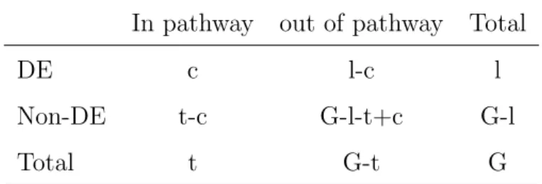
Table 1.2: 2×2 Contingency Table for Pathway Enrichment Analysis

In pathway out of pathway Total

DE c l-c l

Non-DE t-c G-l-t+c G-l

Total t G-t G

was then counted as a 2×2 contingency Table (Table 1.2). The p-value for enrichment of a pathway was calculated by testing the independence of the 2×2 contingency Table using Fisher’s exact test. The null and alternative hypothesis for the Fisher’s exact test is:

H0 : p1 =p2 and Ha : p1 > p2, where p1 and p2 are the probability of DE genes inside and

outside of the pathway. In the Fisher’s exact test, suppose a total number ofG genes in the genome were considered, among them t genes were in the pathway, l genes were contained in the biomarker list and c genes were common to the target pathway (gene set) and the biomarker list (shown in Table 1.2). The p-value of the pathway enrichment was calculated from a hypergeometric distribution by p=∑min(_x=cl,t)(_xt)(G_l−−_ct)/(G_l).

1.5.2 Kolmogorov-Smirnov (KS) Test

The Kolmogorov-Smirnov test (KS test) is a nonparametric test for the equality of contin-uous, one-dimensional probability distributions that can be used to compare a sample with a reference probability distribution (one-sample KS test), or to compare two samples (two-sample KS test). The two-(two-sample KS test is one of the most useful and general nonparametric methods for comparing two samples, as it is sensitive to differences in both location and shape of the empirical cumulative distribution functions of the two samples, so it was widely used in pathway enrichment analysis[91, 61]. Specifically, the p-values calculated from individual analyses or meta-analyises for assessing the DE genes are classified into two categories, in the pathways (P) and out of pathway (PC_{). Let p}

(1), p(2),· · · , p(n) and ˜p(1),p˜(2),· · · ,p˜(m) denote

distribution functions, ˆFP(x) and ˆFPC(x) for P and PC can be defined as: ˆ FP(x) =              0, if x < p(1) k/n, p(k)≤x < p(k+1) for k= 1,2,· · · , n−1 1, if x≥p(n) and ˆ FPC(x) =              0, if x <p˜(1) k/m, p˜(k)≤x <p˜(k+1) for k = 1,2,· · · , m−1 1, if x≥p˜(m)

LetFP andFPC denote the population distribution forP andPC, respectively. The one-sided two sample KS test can be defined based on the formula:

TKS = sup x

(FP(x)−FPC(x)) (1.29) in which the null hypothesis and the alternative hypothesis are:

H0 : FP(x) = FPC(x) for all X (1.30)

Ha : FP(x)≥FFC(x) for all x (1.31)

FP(x)> FPC(x) for some x (1.32) Under the null hypothesis, the rejection region has the form of TKS > Kα at level of α. Rejection of H0 means that P is stochastically less than PC (the CDF of P lies above and

hence to the left of that for PC). In other words, the p-values of genes in the pathway P

are stochastically less than the p-values of genes outside of pathwayPC_{. This indicates that} genes in the pathway P have a stronger association with phenotype than genes from outside of the pathway PC_{; thus, the pathway is of interest. Small p-value associated with KS test} indicates a good performance of the methods.

2.0 A SYSTEMATIC STATISTICAL APPROACH TO INTEGRATE WEAK-SIGNAL MICROARRAY STUDIES ADJUSTED FOR CONFOUNDING VARIABLES WITH APPLICATION TO MAJOR

DEPRESSIVE DISORDER

2.1 MOTIVATIONS

Microarray technology enables researchers to examine the expression of thousands of genes in parallel. Differentially expressed (DE) gene detection is one of the most common anal-yses in microarray data. In such an analysis, genes differentially expressed under multiple conditions are detected and are used for generating further biological hypotheses, developing potential diagnostic tools, or investigating therapeutic targets. The extensive applications of microarray technology have led to an explosion of gene expression profiling studies publicly available. However, the noisy nature of microarray data, together with small sample size in each study, often results in inconsistent biological conclusions [28, 92, 107]. Therefore, meta-analysis, a set of statistical techniques to combine multiple studies under related re-search hypotheses, has been widely applied to microarray analysis to increase the reliability and robustness of results from individual studies. In the literature, three major categories of meta-analysis methods have been applied to genomic meta-analysis: combining effect sizes [15, 66] , combining p-values [52, 79, 80] and combining rank statistics [21, 48]. In general, different approaches have different underlying assumptions and pros and cons in the appli-cation [78]. Major depressive disorder is a heterogeneous illness with mostly uncharacterized pathology. Despite many gene expression studies of MDD [3, 53, 85, 88, 87] published, the biological mechanisms of MDD remain mostly uncharacterized [7]. Although biomarkers and pathways have been identified in specific studies, the findings are not consistently

ob-served from study to study. This variability may be due to several factors. Firstly, MDD is thought to be a complex and heterogeneous disease [72], associated with multiple genetic, genomic, post-translational, and environmental factors. Furthermore, patients might have varying disease severity, with some having psychotic features as well as exposure to a variety of medications and dosage levels to control their illness. Secondly, the genetic disease effects are potentially confounded by many covariates, which include (1) demographical variables such as age, gender and race; (2) clinical variables such as anti-depressant drug usage, sui-cide and alcohol consumption; (3) technical variables inherent in the use of post-mortem brain samples, such as the pH level of brain tissues, brain region and postmortem interval (PMI). If the statistical models employed to identify differentially expressed genes fail to incorporate these sources of heterogeneity, not only can this reduce the statistical power, but also it will introduce sources of spurious signals to the gene detection. Finally, sample sizes for these studies are generally small (between 10-25 pairs of MDDs and controls) due to the limited availability of suitable brain specimens and the significant costs associated with their collection. In this paper, we propose a statistical framework to tackle weak signal expression profiles that have small sample size, case-control paired design and confounding covariates in each study. We use a set of five major depressive disorder (MDD) expression profiles as an illustrative example. In the literature, most analyses of similar data struc-ture either ignored the potentially confounding covariates by using paired or unpaired t-test [18, 51, 98] or applied simple linear regression model to incorporate all covariates [67, 76]. The former approach undoubtedly ignored effects from confounding covariates; the latter approach was not efficient or even not applicable when the number of covariates is large and the number of samples in each study is small. In this paper, we will propose a framework that uses a random intercept model (RIM) to account for the case-control paired design and confounding covariates in single study analysis. An improved RIM with gene-specific vari-able selection (namely RIM minP or RIM BIC to be introduced later) will be performed to accommodate the small sample size and relatively large number of covariates in individual studies. We will then apply and compare three popular meta-analysis methods: Fisher’s method [31, 32], inverse variance weighted random effects model [15, 44], and maximum p-value method [50,86, 103]. Our proposed framework is general and applicable in commonly

Table 2.1: Data description of five MDD microarray studies

Study Gender Brain region sample Platform MD1 ACC M ACC 32(16) Affymetrix MD2 ACC M ACC 20(10) Illumina MD3 ACC F ACC 50(25) Illumina MD1 AMY M AMY 28(14) Affymetrix MD3 AMY F AMY 42(21) Illumina

encountered microarray meta-analysis of complex genetic diseases. Simulations considering various correlation structures among disease state, gene expression and covariates will be performed to demonstrate the better performance of this framework. The application of combining five MDD microarray studies also show improved DE gene detection power and superior statistical significance of pathway detection using our proposed method.

2.2 MATERIALS

Description of motivating MDD data:This research is motivated from the meta-analysis of combining five MDD transcriptomic studies. Brain tissues of three patient cohorts (MD1, MD2 and MD3) obtained from different sources at different time were analyzed. For all three patient cohorts, tissues from the anterior cingulated cortex (ACC) brain region were analyzed by microarray experiments independently to generate three microarray studies: MD1 ACC, MD2 ACC and MD3 ACC. Similarly, tissues from the amygdala (AMY) brain region in MD1 and MD3 cohorts were analyzed to generate MD1 AMY and MD3 AMY. Details of the five patient cohorts and microarray studies are available in Table 2.1. In each patient cohort, MDD patients were matched to control patients by three demographic vari-ables: age, sex and race. Three additional clinical variables (alcohol consumption, history of taking anti-depressant drugs and history of committing suicide) and two technical

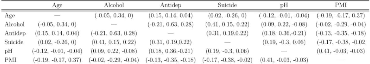
vari-Table 2.2: Pearson correlation between covariates in three MDD cohorts (collinearity evaluation) Age Alcohol Antidep Suicide pH PMI

Age — (-0.05, 0.34, 0) (0.15, 0.14, 0.04) (0.02, -0.26, 0) (-0.12, -0.01, -0.04) (-0.19, -0.17, 0.37) Alcohol (-0.05, 0.34, 0) — (-0.21, 0.63, 0.28) (0.41, 0.15, 0.22) (0.09, 0.22, -0.08) (-0.02, -0.29, -0.04) Antidep (0.15, 0.14, 0.04) (-0.21, 0.63, 0.28) — (0.31, 0.19,0.22) (0.18, 0.36,-0.21) (-0.13, -0.35, -0.18) Suicide (0.02, -0.26, 0) (0.41, 0.15, 0.22) (0.31, 0.19,0.22) — (0.19, -0.3, 0.06) (-0.17, -0.38, -0.02 pH (-0.12, -0.01, -0.04) (0.09, 0.22, -0.08) (0.18, 0.36,-0.21) (0.19, -0.3, 0.06) — (0.41, -0.03, -0.03) PMI (-0.19, -0.17, 0.37) (-0.02, -0.29, -0.04) (-0.13, -0.35, -0.18) (-0.17, -0.38, -0.02) (0.41, -0.03, -0.03) —

ables (pH level of brain tissues and post-mortem interval PMI) were also available for each patient. Among the covariates described above, six variables (age, alcohol, drug, suicide, pH and PMI) are considered potential confounders in the DE gene detection of MDD. These six covariates were not highly correlated in our analysis and thus the collinearity issue does not exist in the linear models below (see Table 2.2).

Data preprocessing, gene matching and gene filtering: Microarray images were scanned and summarized by manufacturers’ defaults. Data from Affymetrix arrays were processed by RMA method and data from Illumina are processed by manufacturer’s soft-ware for probe analysis. When samples in each study were processed in multiple batches, potential batch effects were evaluated and normalizations were performed to correct batch biases when necessary. Probes (or probe sets) were then matched to official gene symbols using Bioconductore package. When multiple probes (or probe sets) matched to an iden-tical gene symbol, the probe that generated the best disease association (by paired t-test) was selected to match to the gene symbol. This selection may cause potential bias but can increase statistical power in such weak-signal data. After genes were matched across five studies, 16,715 unique gene symbols were available across all five studies and intensities were all log-transformed (base 2). Two sequential steps of gene filtering were then performed. In the first step, we filtered out genes with very low gene expression that were identified with small average expression values across majority of studies. Specifically, mean intensities of each gene across all samples in each study were calculated and the corresponding ranks were obtained. The sum of such ranks across five studies of each gene was calculated and genes with the highest 30% rank sum were considered un-expressed genes (i.e. small expression

in-tensities) and were filtered out. Similarly, in the second step, we filtered out non-informative (small variation) genes by replacing mean intensity in the first step with standard deviation. Genes with the lowest 40% rank sum of standard deviations were filtered out. Supplement Figure 1 shows the preprocessing diagram and the number of genes remained in each pre-processing step. Finally, 7,020 matched genes (16715×0.7×0.6 = 7020) in five studies were analyzed.

2.3 METHODS

2.3.1 Single study analysis for DE gene detection

Paired t-test and Wilcoxon signed rank test:As a comparison, paired t-test and Wilcoxon signed rank test were performed. These two methods took into the MDD and control paired design into consideration but ignored the confounding covariates.

Random intercept model (RIM) and fixed effects model (FEM):To account for paired design (MDD samples paired with corresponding controls) and existence of MDD re-lated covariates, we applied a random intercept model (RIM). For a given gene g, we fit the model Ygik =µg+βg0X0ik+ L ∑ l=1 βglXlik+αk+ϵgik, (2.1)

In the model,Ygik was the gene expression value of gene g(≤g ≤G) and samplei(i= 1 for control and 2 for MDD) in pairk(1≤k ≤K). X0ik was the disease label that took value one if the sample was MDD and Zero if sample was a control. Xlik represented values for potential confounding covariate l (1≤≤6; 0-1 binary for alcohol, drug and suicide and numerical for age, pH and PMI). αk was the random intercept from a normal distribution with mean zero and variance τ_g2, which represented the deviation of averaged expression values in the kth pair from the average in the whole population. Finally,ϵgik were independent random noises that followed a normal distribution with mean zero and variance σ_g2. Under this model, βg0

was the disease effect of geneg and was the parameter of major interest. To obtain an MDD-associated biomarker candidate list in a single study analysis, likelihood ratio test (LRT) was used to assess the p-values of testing H0 : βg0 = 0 (vs HA : βg0 ̸= 0). The p-values were then be corrected by Benjamini-Hochberg procedure [8] for multiple comparison.

Fixed effects model (FEM) below ignores the paired design while still considers the covariates in the model. It can be used when diseased and control samples are not paired.

Ygik =µg+βg0X0ik+s L

∑

l=1

βglXlik+ϵgik (2.2) RIM and FEM with variable selection: Although RIM model can effectively ad-just for confounding covariates in DE gene detection, the small sample size (10-25 pairs) and relatively high number of potential confounders (6 covariates) can make the model inefficient and impractical. In this paper, we developed and evaluated two choices of variable selection procedures in the random intercept model (namely, RIM BIC and RIM minP). Specifically, all possible RIM models that included at most two (0, 1 or 2) clinical variables were computed and compared. In RIM BIC, the model with the smallest Bayesian Information Criterion (BIC) [84] value was selected. For RIM minP, we selected the model that yielded the small-est p-value associated with the likelihood ratio tsmall-est for tsmall-esting the disease effectH0 :βg0 = 0.

Conceptually, BIC selected the model with the best model fitting and prediction while minP focused on the model that gave the best statistical significance of the disease effect. This additional variable selection avoided to include more than 2 clinical variables in the model and allowed assessment of biomarkers affected by different sets of covariates in each gene (e.g. gene A is confounded by alcohol while gene B is confounded by drug), which biologi-cally gave more appealing conclusions and interpretations. Similar to RIM model, likelihood ratio test were used to generate p-values of testing H0 :βg0 = 0 in each gene for the selected

model by BIC or minP. These attached p-value numbers were, however, not the true p-values for DE gene detection since they were biased from the variable selection procedure and the type I error control was voided. As a result, we performed a permutation test that randomly permuted the disease labels within each pair to generate a null distribution for p-value as-sessment. Figure 2.1 shows the simulated null distribution from permutation analysis. The skewed distribution deviating from uniform distribution between 0 and 1 showed the need

0.0 0.2 0.4 0.6 0.8 1.0

0

1

2

3

minP: The density plot of p−values under null Density MD1_ACC MD2_ACC MD3_ACC MD1_AMY MD3_AMY Uniform 0.0 0.2 0.4 0.6 0.8 1.0 0.0 0.5 1.0 1.5 2.0

BIC: The density plot of p−values under null Density MD1_ACC MD2_ACC MD3_ACC MD1_AMY MD3_AMY Uniform

Figure 2.1: Simulated null distributions of disease effect p-value in the best model (left: RIM minP; right: RIM BIC) from permutation analysis in the five MDD studies. The result shows bias (deviation from uniform distribution) caused by variable selection.

of the permutation analysis for value correction. Subsequently, the resulting unbiased p-values after permutation correction were then corrected by Benjamini-Hochberg procedure for multiple comparison in each study for DE gene detection. Detailed algorithm of the per-mutation analysis is described in AppendixA. In contrast to RIM minP and RIM BIC, we denote by RIM ALL the RIM model that includes all covariates without variable selection.

Testing significance of interaction terms of each covariate: In the literature, age as well as other covariates has been found to be confounders of the disease effect with significant interaction term in some important biomarkers. [34,39] In other words, the disease effect on gene expression may be affected by age differently in older and in younger cohorts.

Table 2.3: The number of significant interaction terms between disease state and covariates in FEM model and RIM.

FEM RIM MD1 A CC MD2 A CC MD 3 A C C MD1 AMY MD 3 AMY MD1 A CC MD 2 A C C MD3 A CC MD 1 AMY MD3 AMY FDR=0.05 Age 0 0 0 0 0 54 1 0 0 0 pH 0 1 0 0 0 0 7 2 0 0 PMI 0 0 0 0 0 0 2 0 0 0

To evaluate the overall impact of the interaction terms in each covariate, we performed the following simple linear model

Ygik =µg+βg0X0ik+βglXlik+γglX0ikXlik+ϵgik (2.3)

, and random intercept model

Ygik =µg +βg0X0ik+βglXlik+γglX0ikXlik+αk+ϵgik, (2.4)

where the notations were the same as in FEM model and RIM model with only one covariate

l included and a corresponding interaction term involved. We performed likelihood ratio test for H0 : γgl = 0 to test the statistical significance of the interaction term of gene g and covariate l. Table 2.3 summarizes the number of significant interaction terms in the genome of each covariate. The result shows that the interaction terms between each covariate (Age, pH or PMI) and MDD were not significant in most of the genes under false discovery rate FDR = 5% (Benjamini-Hochberg correction). As a result, we did not consider the interaction terms in our RIM models hereafter.