University of South Florida
Scholar Commons
Graduate Theses and Dissertations Graduate School
2009
Mixture distributions with application to
microarray data analysis
O'Neil Lynch
University of South Florida
Follow this and additional works at:http://scholarcommons.usf.edu/etd Part of theAmerican Studies Commons
This Dissertation is brought to you for free and open access by the Graduate School at Scholar Commons. It has been accepted for inclusion in Graduate Theses and Dissertations by an authorized administrator of Scholar Commons. For more information, please contact
Scholar Commons Citation
Lynch, O'Neil, "Mixture distributions with application to microarray data analysis" (2009).Graduate Theses and Dissertations.
Mixture Distributions with Application to Microarray Data Analysis
by
O’Neil Lynch
A dissertation submitted in partial fulfillment of the requirements for the degree of
Doctor of Philosophy
Department of Mathematics and Statistics College of Arts and Sciences
University of South Florida
Co-Major Professor: Kandethody Ramachandran, Ph.D. Co-Major Professor: Wonkuk Kim, Ph.D.
Chris Tsokos, Ph.D. Tapas Das, Ph.D.
Date of Approval: September 4, 2008
Keywords: Likelihood ratio test; Modified likelihood, Penalized likelihood; Asymptotic chi-square distribution; Consistency
c
Dedication
Acknowledgements
It is a great pleasure for me to express my profound respect, gratitude, and admiration for my major supervisor Dr. K. Ramachandran and co-major supervisor Dr. W. Kim. They have given unstintingly of their time, advise, and encouragement ever since they both undertook the task to make me further understand the fields of microarray data analysis and mixture distribution.
I also would like to thank the other members of my committee namely Dr. C. Tsokos, and Dr. T. K. Das who all have given of their time and have always encouraged me to do my best. The staff at the Department of Mathematics and Statistics is deserving of my thanks for the help and advice they have given me over the years.
I owe thanks to my family and a large number of friends for the encouragement and complete understanding in my quest to excel in the field of Statistics.
Table of Contents
List of Figures iv
List of Tables vi
Abstract viii
1 Introduction 1
2 Microarray Data and Some Statistical Analysis 4
2.1 DNA Microarray Experiments . . . 4
2.1.1 Genetic Background . . . 4
2.1.2 cDNA Microarray Experiment . . . 5
2.1.3 Oligonucleotide Microarray Experiment . . . 6
2.2 Some Statistical Challenges With Analyzing Microarray Data . . . 7
2.3 Methods of Analyzing Microarray Data . . . 8
2.3.1 Cluster Analysis . . . 8
2.3.2 The T-Test . . . 10
2.3.3 Regression Model . . . 10
2.3.4 Significance Analysis of Microarrays (SAM) . . . 11
2.3.5 Mixture Model Method (MMM) . . . 13
2.3.6 A Mixture Model Approach Using P-Value . . . 15
2.4 Conclusion . . . 18
3 Finite Mixture Distribution 19 3.1 Definition and Preliminary . . . 20
3.1.2 Mean and Variance of Mixtures . . . 22
3.1.3 Comparison of Two Groups: Iris Data . . . 24
3.2 Parameter Estimation . . . 31
3.2.1 Expectation Maximization Algorithm . . . 31
3.2.2 Robust Parameter Estimation . . . 38
3.2.3 Penalized Maximum Likelihood Estimator for Normal Mixture Models . . . 41
3.3 Estimating the Number of Components g . . . 44
3.3.1 Simulation Approach . . . 45
3.3.2 Modified Likelihood Ratio Test for Homogeneity in Finite Mixture Models . . . 48
3.3.3 Regularity Conditions . . . 52
3.4 Box-Cox transformation . . . 53
3.5 Conclusion . . . 54
4 The Penalized Modified Likelihood for Normal Mixture Model 56 4.1 Penalized Modified Likelihood . . . 57
4.2 Parameter Estimation of Penalized Modified Likelihood . . . 58
4.2.1 Inverse Gamma Penalty Function forσ . . . 60
4.2.2 Inverse Chi-Square Penalty Function for σ . . . 62
4.3 Consistency and Asymptotic Normality . . . 64
4.3.1 Preliminary Results . . . 65
4.3.2 Main results . . . 73
4.4 Conclusion . . . 75
5 Penalized Modified Likelihood Approach to Microarray Data Analysis 76 5.1 Penalized Modified Mixture Model (PMMM) . . . 77
5.2 PMMM Simulated Null Distribution . . . 77
5.3 Simulating Microarray Data . . . 81
6 ModifiedP-Value Approach to Microarray Data Analysis 91
6.1 The modified P-Value Approach . . . 91
6.2 Simulated Null Distribution of the Modified P-Value Approach . . . 95
6.3 Application of Modified P-Value to Simulated Microarray Data . . . 96
6.4 Application of Modified P-Value to simulated Prostate Data . . . 98
6.5 Application of Modified P-Value to the Prostate Data . . . 99
6.6 Conclusion . . . 101
7 Summary and Concluding Remarks 102
References 105
List of Figures
3.1 Histogram of Sepal length of the two species of flowers . . . 25
3.2 Q-Q plots of Sepal lengths for versicolor flowers . . . 26
3.3 Q-Q plots of Sepal lengths for verginica flowers . . . 26
3.4 Histogram and known mixture distribution . . . 27
3.5 Histogram and estimated mixture distribution . . . 28
3.6 Histogram with known and estimated mixture distribution . . . 29
3.7 Graphical representations of two component normal with equal variance . . . 30
3.8 Histogram, heteroscedastic and homoscedastic fit for simulated data from the mixture 0.5φ(y|4,1) + 0.5φ(y|8,1) . . . 41
3.9 Histogram, heteroscedastic and homoscedastic fit for simulated data from the mixture 0.5φ(y|4,1) + 0.5φ(y|8,2) . . . 42
5.1 Histograms of z, Z and fitted models for the simulated data . . . 83
5.2 The likelihood ratio statistic as a function of Z value for the simulated data . . . 85
5.3 The values of FDR from our method and SAM for the simulated data . . . 85
5.4 Histograms of z, Z and fitted models for the rat data . . . 87
5.5 The likelihood ratio curve for the rat data . . . 89
5.6 The values of FDR from our method and SAM for the rat data . . . 89
6.1 Various Beta Distributions . . . 94 6.2 Histogram of p-value and beta mixture distributions for
6.3 Histogram of p-value and beta mixture distributions for
simulated prostate data . . . 98 6.4 Histogram of p-value and beta mixture distributions for
List of Tables
3.1 Summary statistics of data. . . 24 5.1 Mean, variance and percentiles for the penalized modified
likelihood, based on 1000 replicates for each sample for testing
the hypothesis a 1-component against 2-components. . . 79 5.2 Mean, variance and percentiles for the penalized modified
likelihood, based on 1000 replicates for each sample for testing
the hypothesis 2-components against 3-components. . . 80 5.3 Hypothesis test for the number of components for the fitted
normal mixture models of z and Z, for the simulated
microarray data. . . 82 5.4 Values of TP, FP and FDR from PMMM for the simulated data . . . 84 5.5 Values of TP, FP and FDR from SAM for the simulated data . . . 84 5.6 Hypothesis test for the number of components for the fitted
normal mixture models of z and Z, for the rat data. . . 86 5.7 Values of TP, FP and FDR from PMMM for the rat data . . . 88 5.8 Values of TP, FP and FDR from SAM for the rat data . . . 88 6.1 Mean, variance and percentiles for the likelihood ratio test for
the modified p-value, based on 1000 replicates for each sample for testing the hypothesis a uniform against a uniform and
6.2 Mean, variance and percentiles for the likelihood ratio test for the modified p-value, based on 1000 replicates for each sample for testing the hypothesis a uniform against a uniform and
two beta distributions. . . 96 6.3 Hypothesis test for the number of components for the fitted
Mixture Distributions with Application to Microarray Data Analysis
O’Neil Lee Lynch
ABSTRACT
The main goal in analyzing microarray data is to determine the genes that are dif-ferentially expressed across two types of tissue samples or samples obtained under two experimental conditions. In this dissertation we proposed two methods to determine differentially expressed genes. For the penalized normal mixture model (PMMM) to de-termine genes that are differentially expressed, we penalized both the variance and the mixing proportion parameters simultaneously. The variance parameter was penalized so that the log-likelihood will be bounded, while the mixing proportion parameter was penalized so that its estimates are not on the boundary of its parametric space. The null distribution of the likelihood ratio test statistic (LRTS) was simulated so that we could perform a hypothesis test for the number of components of the penalized normal mixture model. In addition to simulating the null distribution of the LRTS for the pe-nalized normal mixture model, we showed that the maximum likelihood estimates were asymptotically normal, which is a first step that is necessary to prove the asymptotic null distribution of the LRTS. This result is a significant contribution to field of normal mixture model.
The modified p-value approach for detecting differentially expressed genes was also discussed in this dissertation. The modified p-value approach was implemented so that a hypothesis test for the number of components can be conducted by using the modified
parametric space. The null distribution of the (LRTS) was simulated so that the num-ber of components of the uniform beta mixture model can be determined. Finally, for both modified methods, the penalized normal mixture model and the modified p-value approach were applied to simulated and real data.
1 Introduction
In recent years microarray technology has made it possible to simultaneously analyze thousands of genes. Although an enormous volume of data is being produced by microar-ray technologies (Schena et al., 1995; DeRisi et al., 1997; Hughes et al., 2001; Lockhart et al., 1996), one remaining challenge is how to analyze and interpret the large amounts of data. A major challenge is to detect genes with differentially expressed profiles under two different experimental conditions, which may refer to samples drawn from two types of tissues, tumors or cell lines, or at two time points during important biological processes. Many of the methods used for such analysis, including the method of identifying genes with fold changes are known to be unreliable because in such methods the statistical variability of the data is not properly addressed [8]. While various parametric
meth-ods and tests such as the two-sample t-test [12] and regression model have been applied
for microarray data analysis, strong parametric assumptions made in these methods as well as strong dependency on large sample sets restrict the reliability of such techniques in microarray problems where only a small number of replications are available. The non parametric statistical methods, including the Empirical Bayes (EB) method [14], the significance analysis for microarray data (SAM [39]) and mixture model method (MMM) [27, 42, 25] have been applied to microarray data analysis. It is claimed and ar-gued that the new extensions of the (MMM) are among the available methods producing biologically-meaningful results [27, 43].
In this dissertation we extended the mixture model method (MMM) by penalizing the mixing proportions and the component variances simultaneously. The mixing proportion was penalized so that a modified likelihood ratio test similar to that of Chen et al. (2001,
in the existence of the MLE’s. In a similar fashion the p-value approach (Allison et al. (2002)) for the detection of differentially expressed genes of microarray data was also
modified. For thep-value approach only the mixing proportion was modified so that the
MLE of the mixing proportion was not on the boundary of its parametric space. This modification was done so that a modified likelihood ratio test similarly to what was done by Chen et al. may be implemented so that we may test the hypothesis for the number of components.
This dissertation is organized as follows. Chapter 2 describes in some detail the genetic background of DNA and two of the leading microarray experiments, cDNA and Oligonucleotide. In Chapter 2 we also discussed some of the statistical challenges we have in analyzing microarray data and gives a description of some of the methods used to analyze microarray data. The methods that were discussed are (1) Cluster analysis (2) T-test (3) Regression analysis (4) Significant analysis of microarray (SAM) (5) Mixture
model method (MMM) and (6) A p-value approach for detecting differentially expressed
microarray data.
In Chapter 3 we present the theory of finite mixture methods and discussed how the parameters can be estimated by (1) expectation maximization algorithm (EM) and (2) the robust parameter estimation - which is of interest if the data contains outliers. One of the challenges of finite mixture distributions is to determine the number of components therefore we discussed some techniques used to determine the number of components which are namely AIC, BIC, simulation and the modified likelihood ratio test. The box-cox transformation for distinquishing skewed distributions from commingled distributions was also presented in chapter 3.
The penalized modified approach will be discussed in chapter 4. The estimators of the parameters of the penalized normal mixture model when both the variance and mixing proportion were simultaneously penalized was illustrated. The evaluation of the estimators for the two penalty functions for the variance, the inverse gamma and inverse chi-square distributions were addressed. The asymptotic property namely asymptotic normality of the normal mixture model was also proved in Chapter 4. Chapter 5 discussed the applications of the penalized/modified approach of the normal mixture model to detecting differentially expressed genes and illustrated its applications to simulated and
real data. The results of the penalized/modified normal mixture model approach were compared to that of SAM and was shown to out perform SAM.
Chapter 6 discussed the modified p-value approach for detecting differentially
ex-pressed genes. Similar to the work done in Chapter 6 we applied our method to
simu-lated and real data. The motivation for modifying the p-value approach of Allison et al.
was that the MLE of the mixing proportion was on the boundary point of its parametric space, therefore we applied the technique of Chen et al., that is, we applied a penalty function for the mixing proportion so that the MLE of the mixing proportion will not be on the boundary points of its parametric space. The conclusions of this study were summarized in Chapter 7.
2 Microarray Data and Some Statistical Analysis
2.1 DNA Microarray Experiments
2.1.1 Genetic Background
The double-stranded molecules deoxyribonucleic acid (DNA) (Watson and Crick, 1953) contains all the genetic information of living organisms. Each strand or helix of DNA is a chain of nucleotides that consists of a sugar, a phosphate and a nitrogenous base molecule. The information in DNA is stored as a code made up of four chemical bases: Adenine (A), Guanine (G), Cytosine (C) and Thymine (T). These four bases are responsible for the DNA molecule having four distinct types of nucleotides. The bases are coupled in the following manner: A with T and C with G, by a hydrogen bond which is called complementary base pairing. The nucleotides are arranged in two long strands that form a spiral called a double helix. The double helix structure of DNA is similar to a ladder, with the base pairs forming the ladder’s rungs and the sugar and phosphate molecules forming the vertical sidepieces of the ladder.
In cells, genes consist of a long strand of DNA that contains a promoter, which controls the activity of a gene. Additionally, all living cells contain chromosomes, that are, large pieces of genes containing hundreds or thousands of genes, each of which specifies the composition and structure of a protein (or several related proteins). The workhorse molecules of the cell are protein polymers of amino acids which are responsible for cellular structure, producing energy and important biomolecules like DNA and proteins, and for reproducing the cell chromosomes. The cohort of chromosomes are almost the same in every cell in an organism, and contains the same repertoire of proteins. However, cells have remarkably distinct properties, such as the difference between human eye cells, hair cells, and liver cells; these distinctions are the result of differences in the abundance,
distribution, and state of the cell proteins.
When a gene is active, the coding and non-coding sequence is copied in a process called transcription, producing messenger RNA (mRNA) which is a copy of the gene’s information. The mRNA, a small and relatively unstable nucleic acid polymers, can then direct the synthesis of proteins through the genetic code. However, mRNAs can also be used directly, for example as part of the ribosome. The resulting molecules from the gene expression, mRNA or protein are known as gene products. There is therefore a logical connection between the state of a cell and the details of its protein and mRNA composition.
Whereas it remains difficult to measure the abundance of a cell’s proteins, DNA mi-croarray makes it possible to quickly and efficiently measure the relative representation of each mRNA species in the total cellular mRNA population, or in more familiar terms, to measure gene expression levels. There are several types of microarray systems including the cDNA microarray (Schena et al., 1995; DeRisi et al., 1997: Hughes et al., 2001) and oligonucleotide array (Lockhart et al., 1996).
2.1.2 cDNA Microarray Experiment
In this experiment, the cDNA sequence corresponding to a set of genes pertinent to the biological question under investigation are obtained and printed onto a glass slide or substrate using a robotic arrayer. Second, the sample RNA is isolated, a critical step in the experiment in order to ensure that a sufficient amount of each cDNA clone is printed on the array where each clone is amplified by a technique called polymerase chain reaction (PCR). In practice the printed amount of cDNA is not the same, therefore the cDNA on the array, which is a double-stranded probe, needs to be denatured and this is achieved by heating the array so that a target cDNA can bind to it.
In the third step the cDNA is synthesized, a procedure that also involves labeling the isolated mRNA from the biological samples. Usually in the most current cDNA microarray experiments, cDNAs from the experimental and reference samples are labeled with red-fluorescent dye, Cy5 and green-fluorescent dye, Cy3 respectively, mixed and
Tagging, Direct Incorporation Labeling and Amino-Modified Nucleotide. Nguyen et al. (2002), Wong et al. (2001) and Stears et al. (2000) discuss the advantages and disadvantages of these methods.
Fourth, the labeled probe cDNA is hybridized to target the cDNA on the microarray. That is, if a particular gene is expressed in the target cell, where the cDNAs correspond-ing to this gene are found in the target cDNA pool, these cDNAs will bind with the complementary cDNA probes printed on a specific spot on the microarray. Hybridiza-tion refers to the binding ability of two complementary DNA strands by the base-pairing rule thus reforming the DNA double helix.
Finally, the hybridization results are imaged and analyzed using a fluorescent micro-scope, the log(red/green) intensities of mRNA hybridization at each site is measured. The result is tens of thousands of gene expressions, typically ranging from -4 to 4, which is a measure of the expression level of each gene in the experimental sample relative to the reference sample. Positive values indicate higher expression in the target versus the reference, and vice versa for negative values.
2.1.3 Oligonucleotide Microarray Experiment
Another widely used microarray technology is high density oligonucleotide arrays known as Affymetrix (Lockhart et al., 1996). This method is based on the fact that each gene is represented by 14 to 20 features (Lipshutz et al., 1999). for example, Affymetrix array used 20 features. Each feature is a short sequence of nucleotides, an oligonucleotide, and it is a perfect match (PM) to a segment of the gene. Paired with the 20 PM oligonu-cleotides to the gene sequence are 20 other oligonuoligonu-cleotides having the same sequence corresponding to the 20 PMs except for a single mismatch (MM) at the central base of the nucleotide. When the gene is expressed in the cell sample, high intensity is expected for the PM feature and low intensity for the MM feature. Given the 20 PM and MM feature pairs for the gene, many methods have been proposed to quantify the expression level of the gene. For example, Affymetrix originally proposed the average difference
x = avg{dk = (P Mk−MMk), k = 1,2, . . . ,20 = K} to quantify expression level of a gene in a particular array. The average is usually based only on the differences,dk, with
3 standard deviations from the mean of d(2), . . . , d(K−1), where d(k) is the kth smallest
difference, but there are various other ways to filter the outliers, Efron et al. (2001) suggested x = avg{dk = log(P Mk)−clog(MMk), k = 1,2, . . . ,20} for several different
scale factors c. Naef et al. (2001) proposed to use only the PM features. In an attempt
to obtain more sensitive measure of gene expression, Li and Wong (2001) proposed a model-based estimate of the expression level using the least square method. The method for sample labeling and image processing in the Affymetrix arrays are found in Lockart et al. (1996). Refer to ”The Chipping Forecast” (Lander et al., 1999) for more details on cDNA microarrays and oligonucleotide chips.
2.2 Some Statistical Challenges With Analyzing Microarray Data
Microarray technologies allow scientists to monitor the mRNA transcript levels of thou-sands of genes in a single experiment. However, the tremendous amount of data that is obtained from microarray studies presents challenges for data analysis. One challenge in the development of statistical methods for microarray data analysis is that sample sizes under two different experimental conditions are typically small. We can depict this situation by defining the data as follows: for each genei, i= 1,2, . . . , N, we have expres-sion levels (Yi1, . . . , Yim) from m microarrays under condition 1, and (Yi,m+1, . . . , Yi,m+n) fromn arrays under condition 2. Usually the total number of genes N is large (>1000) whereas the number of replications, m and n are small (typically< 20).
Since statisticians are primarily interested in genes that are differentially expressed across two different experimental conditions, which may refer to samples drawn from two types of tissues, tumors or cell lines, or at two time points during important biological processes, we need to make an adjustment for the type I error rate when doing simul-taneous hypothesis tests. This adjustment is done by means of the Bonferroni method,
to deal with multiple comparisons. If we use α as the significance level then the test or
gene specific significance level for a two sided test is therefore α∗ =α/2n.
Investigators may need to have the answer for the following question ”Is the difference in expression level for a particular gene statistically significant?” However, there are a
1. Is there statistically significant evidence that any of the genes under study exhibit a difference in expression across the conditions?
2. What is the best estimate of the number of genes for which there is a true difference in gene expression?
3. What is the confidence interval around that particular estimate?
4. If we set some threshold for which we expect particular genes to beinteresting and
worthy of follow-up study, what proportion of those genes are likely to be genes for which there is a real difference in expression and what proportion are likely to be false leads?
5. What proportion of those genes not declared ”interesting”are likely to be genes for which there is a real difference in expression (i.e., misses or false negatives)? In analyzing microarray data the assumptions made are (1) For each gene, the measure-ments of gene expression have a finite population mean and variance; (2) For each gene under study, there is a measure of expression level available for each sample and this measure has sufficient reliability and validity (i.e. the measurements of the expression levels are a true reflection of the true state of nature); (3) The most important assump-tion that is made is that gene expression levels across the two groups are independent - which implies that we may able to evaluate the likelihood function which will become important later in this dissertation.
2.3 Methods of Analyzing Microarray Data
2.3.1 Cluster Analysis
One method used in the analysis of microarray data is Cluster analysis. Cluster analysis groups genes or samples into ”clusters” based on similar expression profiles and provides clues to the function or regulation of genes or similarity of samples via shared cluster membership [34, 35, 18]. Several clustering methods have been usefully applied to an-alyzing genome-wide expression data and can be classified largely into three categories. The three-based approach uses distance measures between genes such as correlation
co-efficients to group genes into a hierarchical tree [15]. The second category clusters genes so that within-cluster variation is minimized and between-cluster variation is maximized [34, 35]. The third category group genes into blocks, in which the correlation is maxi-mized and between which the correlation is minimaxi-mized [3]. The power of cluster analysis in the analysis of microarray data lies in discovering gene transcripts or samples that show similar expression profiles. However, identification of ”like” groups is not necessar-ily the objective in a microarray study, because the interest is to discover genes that are differentially expressed between predefined sample groups, such as normal versus cancer-ous tissues.
Data
Let Yik be the expression level of gene i in array k (i = 1, . . . , N;k = 1, . . . , m, m+ 1, . . . , m+n). Suppose that the first m and the last n arrays are both obtained under two different conditions, that is Yi(1) = (Yi1, . . . , Yim) and Yi(2) = (Yi,m+1, . . . , Yi,m+n). Since we are interested to determine which genes are differentially express betweenYi(1)
and Yi(2), we let Yik =ai+bixk, (2.3.1) where xk = 1 for 1≤k ≤m 0 for m+ 1≤k ≤m+n.
Therefore the mean expression levels of geneiunder the two conditions are ai+bi and ai respectively. Hence to determine the genes that are differentially expressed is equivalent to testing the hypothesis
H0 : bi = 0, there is no gene with altered expression
H1 : bi 6= 0, otherwise (2.3.2)
2.3.2 The T-Test
There are several versions of the two-samplet-test, depending on whether the sample size
(i.e m and n) is large and whether it is reasonable to assume that the gene expression
levels have an equal variance under the two conditions. Bothm and nare usually small,
and there is evidence to support unequal variance (Thomas et. al. 2001), we will only
discus the t-test with two independent small Normal samples with unequal variances.
Let the sample means and variances of Yik for gene i under the two conditions be
¯ Yi(1) = Pm k=1Yik m , Y¯i(2) = Pm+n k=m+1Yik n (2.3.3) and s2 i(1) = Pm k=1(Yik−Y¯i(1))2 m−1 , s2i(2) = Pm+n k=m+1(Yik−Y¯i(2))2 n−1 . (2.3.4) The t-statistic is Zi = ¯ Yi(1)−Y¯i(2) q s2 i(1) m + s2 i(2) n , (2.3.5)
Under the normality assumption for Yik, Zi approximately has a t-distribution with
degrees of freedom dj = ³s2 i(1) m + s2 i(2) n ´2 ³ s2i(1) m ´2 m−1 + ³ s2i(2) n ´2 n−1
This t-test was proposed by Welch (1947). Its method of calculating the degrees of
freedom is similar to the idea of the Satterthwaite approximation.
2.3.3 Regression Model
The regression model estimates the values of (ai, bi) using the weighted least square
estimator. V ar(ˆbi) = ³s2 i(1) m ´³m−1 m ´ + ³s2 i(2) n ´³n−1 n ´ ,
and the estimate of ˆbi = ¯Yi(1)−Y¯i(2). Therefore the test statistics is
Z0 i = ˆbi V ar(ˆbi) = q Y¯i(1)−Y¯i(2) s2 i(1) m mm−1 + s2 i(2) n n−n1 . (2.3.6)
This test statistic compares well with that of the t-test. In the case of thet-test the test statistic is Zi = ¯ Yi(1)−Y¯i(2) q s2 i(1) m + s2 i(2) n , (2.3.7)
where ¯Yi(1),Y¯i(2), s2i(1) and s2i(2) are defined as in (2.3.3) and (2.3.4). Note that the two
tests are the same asm, n→ ∞, however in microarray data analysis bothm, nare small,
which makes the t-test better because of the unbiasedness of its variance estimator. Note that the strong parametric assumptions that needs to be made to use both the t-test and the regression approach is often times violated for microarray data analy-sis. Therefore, the Significance Analysis of Microarrays (SAM) is an important method developed for microarray data analysis that seeks to over theses strong parametric as-sumptions.
2.3.4 Significance Analysis of Microarrays (SAM)
The significance analysis of microarrays (SAM) is one statistical technique for finding significant genes in a set of micoarray experiments. It was proposed by Tusher, Tibshirani and Chu [39]. This approach was based on analysis of random fluctuations in the data. However, even for a given level of expression, the fluctuations were gene specific. To account for gene-specific fluctuations, a statistic based on the ratio of change in gene expression to standard deviation in the data for that gene was defined. The ”relative difference” d(i) in the gene expression is:
where ¯Yi(1) and ¯Yi(2) are defined as the average expression levels of the ith gene from
conditions 1 and 2, respectively. The ”gene-specific scatter”s(i) is the standard deviation of repeated expression measurements:
s(i) = v u u t1/m+ 1/n m+n−2 ³Xm k=1 (Yik−Y¯i(1))2+ mX+n k=m+1 (Yik−Y¯i(1))2 ´ (2.3.9)
where m and n are the numbers of measurements in conditions 1 and 2 respectively.
In order to compare values of d(i) across all genes, the distribution ofd(i) should be independent of the level of gene expression. At low expression levels, variance ind(i) can be high because of small values ofs(i). To ensure that the variance ofd(i) is independent
of the gene expression, a small positive constant s0 (exchangeability factor) was added
to the denominator of equation (2.3.8). The coefficient of variation ofd(i) was computed as a function ofs(i) in moving windows across the data. The value fors0 was chosen to
minimize the coefficient of variation.
To minimize the effects of potential confounders between the conditions, the data
was analyzed by taking B sets of permutations. For each permutation b the statisticd∗b
i and the corresponding order statisticsd∗b
(1) ≤d∗(2)b . . .≤d∗(Nb)was computed. The expected
relative difference, ¯di = P
bd∗ib
B , was defined as the average over the set ofB permutations.
To identify potentially significant changes in expression levels, they used a scatter plot of the observed relative differenced(i) versus the expected relative difference ¯di. For a fixed threshold ∆, starting at the origin, and moving up to the right find the firsti=i1
such thatdi−d¯i >∆. All genes passi1 are called ”significant positive”. Similarly, start
at the origin, move down to the left and find the first i =i2 such that ¯di−di >∆. All genes passi2are called ”significant negative”. For each ∆ the upper cutoff point cutup(∆) was defined as the smallestdi among the significant positive genes, and similarly defining the lower cutoff point cutlow(∆).
To determine the number of falsely significant genes generated by SAM, the total number of falsely significant genes corresponding to each permutation was computed by
counting the number of genes that exceeded the cutoffs cutup(∆) and cutlow(∆). The
estimated number of falsely significant genes was the median (or 90th percentile) of the
false positive (F P). This information will then be used to estimate the false Discovery Rate (F DR)
F DR =π0F P/T P (2.3.10)
where π0 is the true proportion of equivalent expressed (EE) genes in the data set and
T P is the number of total (true) positives discovered from the test statistic, that is,T P
is the total number of genes claimed to be differentially expressed (DE).
2.3.5 Mixture Model Method (MMM)
The mixture model method (MMM) was introduced to handle the problem when a small number of replications under two experimental conditions exist, which is exactly the case for the data in a microarray experiment. The main purpose of the MMM is to estimate the distribution of at-type test statistic and its null statistic using finite normal mixture models, which results in the method being non-parametric. Additionally, the strong parametric assumption made when analyzing microarray when the traditional statistical test is applied is often violated, hence this make the MMM statistically safer because the assumption of normality is not made.
Consider the situation where, for each gene i, i = 1,2, . . . , N, we have expres-sion levels Yi(1) = (Yi1, . . . , Yim) from m microarrays under condition 1, and Yi(2) =
(Yi,m+1, . . . , Yi,m+n) from n arrays under condition 2. Here we need to assume that both
m and n are even integers, this will become obvious later.
The goal is to identify genes such that (Yi1, . . . , Yim) and (Yi,m+1, . . . , Yi,m+n) have different means. This appears to be a two sample comparison however, in microarray data, that has smallmandn with a largeN, renders the traditional statistical tests such
as the t-test or rank-based nonparametric tests, ineffective. One alternative is to draw
statistical inference based on the distributions of quantities related to (Yi1, . . . , Yim) or (Yi,m+1, . . . , Yi,m+n), for 1≤i≤N, to take advantage of the large population size N.
where µi(1) and µi(2) are the mean expression levels for gene i under the two conditions
respectively, andεi(1) andei(2) are independent random errors with means and variances,
such that
E(εi(1)) = E(ei(2)) = 0, V ar(εi(1)) =σi2(1), V ar(ei(2)) =σi2(2),
for anyj = 1, . . . , m, m+1, . . . , m+n andi= 1, . . . , N. Note, we do not assume equality of variance of the gene expression levels, because the varianceσ2
i(c) of gene expression level
depends on the mean expression µi(c). Also, we do not assume µi(1) =µi(2).
The basis of the model is to compare two distributions of two similar statistics (after being suitably standardized) to infer whether some genes are differentially expressed. Let
m and n be even such that pi (qi) is a column vector containing random permutation
of m/2 1’s and m/2 -1’s (n/2 1’s and n/2 -1’s). Let Yi(1) = (Yi1, . . . , Yim) and Yi(2) =
(Yi,m+1, . . . , Yi,m+n) then assume that
zi =
Yqi(1)pi/m+Yi(2)qi/n
s2
i(1)/m+s2i(2)/n
∼f0, (2.3.11)
which does not depend on µi(1) and µi(2) since its mean is 0. Furthermore, suppose that
Zi = Pm k=1Yik/m− Pm+n k=m+1Yik/n q s2 i(1)/m+s2i(2)/n = q Y¯i(1)−Y¯i(2) s2 i(1)/m+s2i(2)/n ∼f1. (2.3.12)
The hypothesis is of the form
H0 : f0 =f1, there is no gene with altered expression
H1 : f0 6=f1, otherwise (2.3.13)
and is valid only if the random errors are independent and their distribution is symmetric about 0. Since m, n > 1 then we can estimate s2
i(1) and s2i(2) using the sample variances
s2 i(1) = Pm k=1(Yik−Yi¯(1))2 m−1 and s2i(2) = Pm+n k=m+1(Yik−Yi¯(2))2
Zi’s are used to estimate f0 and f1 by normal mixture model respectively, which will be
discussed in more details in chapter 3.
To test the null hypothesis H0 that Z is from f0 (which is equivalent to testing the
hypothesis (2.3.13)), we can construct a likelihood ratio test (LRT) based on the following statistic:
LR(Z) = f0(Z)
f1(Z)
. (2.3.14)
A large value ofLR(Z) gives no evidence againstH0, whereas a too small value ofLR(Z)
leads to rejecting H0. With the normal mixture model, it is possible to numerically
determine the rejection region. For any given false positive rate α, we can use the
bisection method [29] to solve
α=
Z
LR(z)<s
f0(z)dz
to obtain the suitable cut off point s. Then the rejection region is RR(α) = {Z :
LR(Z) < s}. We call the method of using the LRT in MMM as MMM-LRT. Similar to
SAM (Tusher et al. 2001), we can estimate the numbers of false positive (F P) and total
(T P) directly. In MMM-LRT, for any given s, we have:
F P(s) = 1 B B X b=1 n(i:LR(zi(b))< s), T P(s) = n(i:LR(Zi)< s)
where n(i) represents the number of genes. In estimating F P, one can also use median,
rather than mean,F P over the permuted data. Based on the estimatedF P andT P, one
can also calculate the false discovery rate as F DR=F P/T P (Benjamini and Hochberg
1995; Storey 2001; Tusher et al. 2001).
2.3.6 A Mixture Model Approach Using P-Value
In is well known that the distribution of the p-values is uniformly distributed on the
H0 there is no difference between the two experiments for theith gene,i= 1, . . . , N, then
the distribution of thep-value can be used to determine the genes that were differentially expressed. The assumption of independence of the gene expression levels across genes was made under the null hypothesis. Additionally, under the alternative hypothesis,
the distribution of p-values will tend to cluster closer to zero than to one, as opposed
to be uniformly distributed under the null hypothesis. Then, the question ”Is there statistically significant evidence that any of the genes under study exhibit a difference in expression across the two experimental conditions?” can be answered by conducting a test to determine if the observed p-values are significantly different from the uniform distribution. This is done by mixture model approach [2].
The mixture model is a g-component of beta distributions β(rj, sj) for j = 1, . . . , g with the parameters rj and sj, where the beta distribution is defined as follows
β(y|r, s) = Γ(r+s)y
r−1(1−y)s−1
Γ(r)Γ(s) .
The reason for the choice of the beta distribution is because of its great flexibility in modeling any shaped distribution on the interval [0,1]. Note that the uniform distribution is a special case of the beta distribution withr=s= 1. The likelihood for the collection
of N, p-values from a model with g components is given as
Lg = N Y i=1 " p1β(yi|1,1) g Y j=2 pjβ(yi|rj, sj) # ,
Therefore the log likelihood for the N p-values can be expressed as
lg = N X i=1 ln " p1β(yi|1,1) + g X j=2 pjβ(yi|rj, sj) # ,
where yi is the p-value for the ith test, p1 is the probability that a randomly chosen test
from the collection of tests is for a gene where there is no population difference in gene expression (i.e., a test of a true null hypothesis), andpj is the probability that a randomly chosen test from the collection of tests is for a gene where there is a population difference in gene expression (i.e., a test of a false null hypothesis). The above model now requires
the calculation of the MLE of the parameters pj, rj and sj through iterative procedure subject to the constraints Pgj=1pj = 1 and 0≤pj ≤1 for allj = 1, . . . , g.
The estimate of the number of genes for which there is a difference in gene expression is evaluated as N(1−pˆ1), where ˆp1 is the MLE of p1. Let T be some threshold below
which the results for particular genes are declared ”interesting”and worthy of follow-up
study, the proportion of those genes that are likely to be genes for which there is a real difference is P( ¯H0,i|yi ≤T) = 1−P(H0,i|yi ≤T) = 1− P(H0,i|yi ≤T) P(yi ≤T) , where P(yi ≤T) = p1T + g X j=2 pj Z T 0 Γ(rj +sj)yrj−1(1−y)sj−1 Γ(rj)Γ(sj) dy
andP( ¯H0,i∩yi ≤T) =p1T. The estimated proportion of genes declared interesting that
are likely to be false leads is simply
P(H0,i|yi ≤T) =
P(H0,i∩yi ≤T)
P(yi ≤T)
.
Similarly the proportion of those genes not declared ”interesting” that are likely to be
genes for which there is a real difference is
P( ¯H0,i|yi ≥T) = 1−P(H0,i|yi ≥T) = 1− P(H0,i|yi ≥T) P(yi ≥T) , where P(yi ≥T) = p1(1−T) + g X j=2 pj Z 1 T Γ(rj +sj)yrj−1(1−y)sj−1 Γ(rj)Γ(sj) dy and P( ¯H0,i∩yi ≥T) = p1(1−T).
2.4 Conclusion
This chapter discussed a few of the methods used to analyze microarray data. An in-troduction to cluster analysis was presented, but, cluster analysis was not an effective method to determine differentially express genes. Hence the need to make use of the
more classical statistical methods such as the t-test and regression analysis. However,
with strong parametric assumptions that will be necessary for microarray analysis, these methods has some limitations. Microarray data are many times consist of a few replica-tions for case and control groups, although the number of genes are usually greater than 1000. The assumption that the genes are independent is one assumption that is typical in the analysis of microarray data. Note that in chapters 3 and 5 the development of the modified approaches use the independence assumption, therefore we are prepared to deal with the consequences of assuming the genes are independent.
The Significance Analysis of Microarrays (SAM) and the Mixture Model Method
(MMM) presented in this chapter uses a t-type statistics to determine the number of
differentially expressed genes. However, the MMM has one advantage in that it is a non-parametric approach. The MMM determines the distributions under the null and alternative and then uses these distributions to determine the number of differentially expressed genes by means of a likelihood ratio test.
The p-value approach of Allision relies on parametric assumptions that are made to
determine the p-values. If the p-values are not valid then its distributions under the
null hypothesis may not be uniform on the interval [0,1]. In discussing the modified
p-value approach presented in chapter 6, we are aware that the t-test used to determine
the p-values must be valid for the modified p-value approach to be valid. However, for
this dissertation we assume all the assumptions are satisfied with respect to the modified
p-value approach.
In addition, to the method used to analyze microarray data, we presented the bio-logical background that the reader needs so that he may fully understand the challenges statisticians have in the analysis of microarray data.
3 Finite Mixture Distribution
In this chapter we will give a brief background on mixture distributions. Mixture models are vital in statistical practice and research because many problems in statistics have mixture structures. Furthermore they are useful in describing complex population with observed or unobserved heterogeneity. Some examples are that human heights may be modeled as a two-component mixture, one component for men and one for women. Sub-structures in galaxy may be modeled as contaminations of big initial galaxy; the evidence of substructures is important in modern galaxy formation theory (Sun, Morrison, Hard-ing and Woodroofe 2002). There are also applications in actuarial science, biological science, econometrics, medicine, agriculture, zoology, population studies and microarray data analysis.
K. Pearson (1894) was the first to study mixture of two normal distributions, where he modeled the mixing of different crab species. Mixture model has become popular because: (1) they provide a simple mechanism to incorporate extra variation and correlation in the model (2) they add model flexibility and (3) they are a natural approach for modeling data that arise in multiple stages or when populations are composed of sub populations. In addition the theory, applications, history and importance of mixture models have been discussed in journal articles, monographs and textbooks. Everitt and Hand (1981), Titterington, Smith and Makov (1985), B¨ohning (1999), and McLachlan and Peel (2000) provided models, statistical methods and references for finite mixtures problems.
3.1 Definition and Preliminary
Definition 3.1.1 A stochastic variable {Yi : 1 ≤ i ≤ n} with density function f(yi|θj)
follows a finite mixture distribution if
Yi ∼ π1fi1(yi|θ1) +π2fi2(yi|θ2) +. . .+πgfig(yi|θg) = g X j=1 πjfij(yi|θj), (3.1.1)
where fi1(yi|θ1), . . . , fig(yi|θg) are g density functions and π1, . . . , πg are called mixing
proportions, satisfying the following properties 0 ≤ πj ≤ 1 and
Pg
j=1πj = 1. The
densitiesfij(y) for j = 1, . . . , g may be continuous or discrete, or a combination of both. From Definition 3.1.1 we observe that finite mixture distribution is the marginal distribution of a random variable which follows different distributions in different
sub-populations of a general population. Therefore, if a population S is defined as
S ={S1, S2, . . . , Sg}, such thatSj∩Sk =∅, j 6=k. Then the distribution in each sub-population is given to be
• In S1 :Y|S1 ∼f1(Y|θ1)
• In S2 :Y|S2 ∼f2(Y|θ2)
• . . .
• In Sg :Y|Sg ∼fg(Y|θg)
Furthermore, let X represent the statistic in each sub-population i.e.,
X =x1, if inS1; X =x2, if inS2; . . . , . . .; X =x3, if inS3.
Then X follows a discrete distribution with support {x1, x2, . . . , xg} and correspond-ing probabilities (weights) {π1, π2, . . . , πg}, that is P(X = xj) = πj for j = 1, . . . , g.
Therefore for the finite mixture Yi ∼ g X j=1 πjfij(yi|θj), we have Yi|(X =xj)∼fij(yi|θj), j = 1,2, . . . , g
where X is denoted as follow,
X ∼ x1 x2 . . . xg π1 π2 . . . πg .
Note the random variable X is called latent because, in most applications, it is not
observed. We now present some examples of finite mixture distributions.
3.1.1 Examples of Mixture Distributions
Example 3.1.2 Normal with common variance, that is,
Y ∼
g
X
j=1
πjN(µj, σ2)
where the parameters for this mixture areθj = (µj, σ2)andπj for j = 1, . . . , g. Note that
Y|(X =µj)∼N(µj, σ2) where X∼ µ1 µ2 . . . µg π1 π2 . . . πg .
Example 3.1.3 Normal with common mean, that is,
Y ∼
g
X
j=1
where the parameters for this mixture are θj = (µ, σj2) and πj for j = 1, . . . , g. Note that Y|(X =σ2 j)∼N(µ, σj2) where X ∼ σ21 σ22 . . . σg2 π1 π2 . . . πg .
Example 3.1.4 Normal with general mean and variance, that is,
Y ∼
g
X
j=1
πjN(µj, σj2)
where the parameters for this mixture areθj = (µj, σj2)andπj for j = 1, . . . , g. Note that
Y|(X1 =µj, X2 =σj2)∼N(µj, σj2) where X = (X1, X2)∼ (µ, σ12) (µ, σ22) . . . (µ, σg2) π1 π2 . . . πg .
3.1.2 Mean and Variance of Mixtures
LetY ∼Pgj=1πijfij(yi|θj) be a random variable that has a mixture distribution. Using the latent variable definition above, the mean and variance have the following known basic probability results for any random variables.
Proposition 3.1.5 E(Y) = E(E(Y|X))
Proposition 3.1.6 V ar(Y) = V ar(E(Y|X)) +E(V ar(Y|X))
This implies that the mean and variance of Examples (3.1.2), (3.1.3) and (3.1.4) are given as: For Example (3.1.2) we have
E(Y) = E(E(Y|X)) = E(X) = g
X
j=1
and V ar(Y) = V ar(E(Y|X)) +E(V ar(Y|X)) = V ar(X) +E(V ar(X)) = g X j=1 πjµ2j − ³Xg j=1 πjµj ´2 +E(σ2) = g X j=1 πjµ2j − ³Xg j=1 πjµj ´2 +σ2. Example (3.1.3) results in E(Y) =E(E(Y|X)) =E(µ) =µ and V ar(Y) = V ar(E(Y|X)) +E(V ar(Y|X)) = V ar(µ) +E(σ2 j) = g X j=1 πjσ2j.
For Example (3.1.4) we have
E(Y) = E(E(Y|X)) =E(X1) = g X j=1 πjµj and V ar(Y) = V ar(E(Y|X)) +E(V ar(Y|X)) = V ar(X1) +E(X2) = g X j=1 πjµ2j − ³Xg j=1 πjµj ´2 +E(σ2 j) = g X πjµ2j − ³Xg πjµj ´2 + g X πjσj2.
3.1.3 Comparison of Two Groups: Iris Data
Here we will use data to illustrate the importance of mixture distribution. The iris data is found in the statistical software package R consisting of 100 sample points of two species of flowers, Versicolor and Virginica was used for this illustrative purpose. For each species the measurements of the sepal length of 50 flowers were reported. It is clear that we have a dataset that is composed of two different populations. Since mixture distribution is applicable in the case where the data has sub-populations, we use this example to illustrate the idea of fitting mixture distribution. Note that in dealing with real life problems one will not have any information as to whether the data is composed of different populations. The histograms for both samples are presented in Figure 3.1.
The summary statistics is given in Table 3.1. For this data we have no evidence that the data is not normally distributed, because the Kolmogorov-Smirnov tests for normality resulted in a p-value > 0.5 for both groups. The Q-Q plots are displayed in Figures 3.2 and 3.3. Additionally, the assumption of equal variance is satisfied because the p-value for the F-test is 0.148.
Table 3.1: Summary statistics of data. Species Sepal Means Sepal Std. Dev.
Versicolor 5.94 0.516
Virginica 6.59 0.636
The known normal mixture distribution using the summary statistics displayed in Table 3.1 is
0.5N(5.94,0.5162) + 0.5N(6.59,0.6362)
and represented graphically in Figure 3.4. However, when a two-component mixture of normals with equal variance was fitted to the data, the following fitted distribution was obtained (Figure 3.5)
0.83N(6.08,0.5262) + 0.17N(7.13,0.5262)
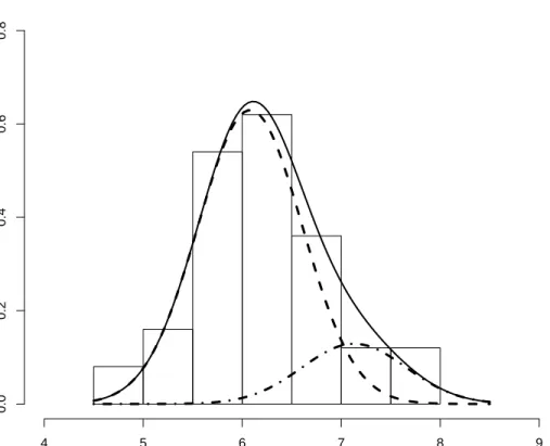
Figure 3.1: Histogram of Sepal length of the two species of flowers Sepal length Versicolor Relative frequency 4 5 6 7 8 0.0 0.2 0.4 0.6 0.8 Sepal length Virginica Relative frequency 4 5 6 7 8 9 0.0 0.2 0.4 0.6 0.8
Figure 3.2: Q-Q plots of Sepal lengths for versicolor flowers −2 −1 0 1 2 5.0 5.5 6.0 6.5 7.0 Normal Q−Q Plot
Expected Normal Value
Veriscolor
Figure 3.3: Q-Q plots of Sepal lengths for verginica flowers
−2 −1 0 1 2 5.0 5.5 6.0 6.5 7.0 7 5 8.0 Normal Q−Q Plot
Expected Normal Value
Figure 3.4: Histogram and known mixture distribution Sepal length Density 4 5 6 7 8 9 0.0 0.2 0.4 0.6 0.8
Dotted lines to the left and right represents the known distributions of versicolor and virginica respectively. The known mixture structure is 0.5N(5.94,0.5162) + 0.5N(6.59,0.6362).
the known mixture model. This example illustrates that the fitted mixture distribution does not necessarily reflect prior known group structures in the data.
In reality the estimated mixture distribution obtained for the illustrative example may be symmetric. The distribution may be bimodal or multimodal in the case where we have more than two components.
Figure 3.5: Histogram and estimated mixture distribution
Sepal length Density 4 5 6 7 8 9 0.0 0.2 0.4 0.6 0.8
Dotted lines to the left and right represents the fitted distributions of versicolor and virginica respectively. The fitted model is given by 0.83N(6.08,0.5262) + 0.17N(7.13,0.5262).
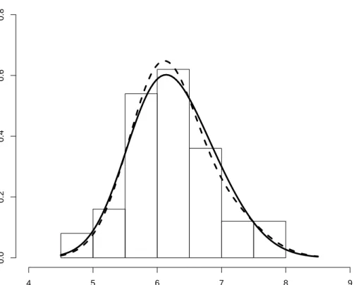
Figure 3.6: Histogram with known and estimated mixture distribution Sepal length Density 4 5 6 7 8 9 0.0 0.2 0.4 0.6 0.8
Dotted line represents the fitted mixture model while the bold line is the known mixture structure.
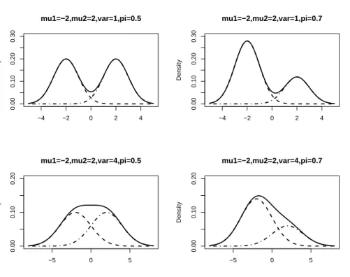
Figure 3.7 depicts that mixtures have very flexible class of models, that is: 1. They are symmetric as well as skewed
Figure 3.7: Graphical representations of two component normal with equal variance πN(µ1, σ2) + (1−π)N(µ2, σ2) −4 −2 0 2 4 0.00 0.10 0.20 0.30 mu1=−2,mu2=2,var=1,pi=0.5 Density −4 −2 0 2 4 0.00 0.10 0.20 0.30 mu1=−2,mu2=2,var=1,pi=0.7 Density −5 0 5 0.00 0.10 0.20 mu1=−2,mu2=2,var=4,pi=0.5 Density −5 0 5 0.00 0.10 0.20 mu1=−2,mu2=2,var=4,pi=0.7 Density
From Figure 3.7 we see that the following proposition below determines the modality of a 2-component mixture if the parameters are known, but in general we do not know
µ1, µ2 and σ.
Proposition 3.1.7 The modality of the 2-component mixture of normals with equal
vari-ance is determined as follows.
If |µ1−µ2| σ
≤2 then the mixture is unimodal ∀ π
3.2 Parameter Estimation
3.2.1 Expectation Maximization Algorithm
This section describes how the parameters of a g-component finite mixture distribution
can be estimated using maximum likelihood estimation (MLE) [10]. Let {Yi}1≤i≤n be
distributed as Yi ∼ π1fi1(yi|θj) +π2fi2(yi|θj) +. . .+πgfig(yi|θg) = g X j=1 πjfij(yi|θj),
wherefij(yi|θj) are density functions ofYi in ag-component mixture. The parameters of interest are that of the density functionsfij(yi|θj) which we denote as a vectorθ and the proportion probability π0 = (π
1, . . . , πg). In short, the mixture distribution parameters can be denoted as a vector ψ0 = (π0, θ0). Let y0 = (y
1, . . . , yg) be a vector of observed values, then the observed likelihood function is given to be:
L(ψ|y) = n Y i=1 ( g X j=1 πjfij(yi|θ) ) , (3.2.2)
additionally, the observed log-likelihood is given by:
l(ψ|y) = n X i=1 ln ( g X j=1 πjfij(yi|θ) ) . (3.2.3)
We now need to maximize the log-likelihood l(ψ|y) with respect to ψ. This is done
by using the Expectation-Maximization (EM) (Dempster et al., 1977) algorithm as an alternative to the Newton-Raphson which involves the calculation of first and second derivatives of l(ψ|y). The EM algorithm was developed for missing observation, in our case we considered the component membership as missing. This can be seen if we define indicators Zij, i= 1, . . . , n,j = 1, . . . , g such that
Therefore we have that P(Zij = 1) =πj, and hence the joint density of Yi and allZij is given by fi(yi, Zi1 =zi1, . . . , Zig =zig) =fi(yi|Zi1 =zi1, . . . , Zig =zig)P(Zi1 =zi1, . . . , Zig =zig) = ( g Y j=1 [fij(yi|θ)]zij ) ( g Y j=1 πjzij ) = ( g Y j=1 [πjfij(yi|θ)]zij )
Therefore the likelihood of the complete data is
L(ψ|y, z) = n Y i=1 g Y j=1 [πjfij(yi|θ)]zij (3.2.4)
and the log-likelihood of the complete data is
l(ψ|y, z) = n X i=1 g X j=1 zij[lnπj + lnfij(yi|θ)]. (3.2.5)
It is therefore obvious that maximizingl(ψ|y, z) (”the complete log likelihood”) is easier
than maximizing l(ψ|y) (”the observe log likelihood”). Note that (3.2.2) and (3.2.3)
are referred to as the observe data likelihood and observe log-likelihood respectively, while (3.2.4) and (3.2.5) are referred to as the complete data likelihood and complete log-likelihood respectively. Instead of maximizing l(ψ|y, z) we maximize E(l(ψ|y, z)|y), which is interpreted intuitively as replacing the missing observationszij by their expected values.
The EM algorithm acts iteratively, in the sense that, starting from a ”first guess estimate” (starting value) ψ(0) for ψ, a series of estimates ψ(t) is constructed, which
converges to the MLE ˆψ of ψ
ψ(0) →ψ(1) →. . .→ψ(t)→ψ(t+1) →. . .→ψ(∞)= ˆψ
Definition 3.2.1 The E-step is the calculation ofQ(ψ|ψ(t)) =E(l(ψ|y, z)|y, ψ(t)).
Definition 3.2.2 The M-step is defined as the maximization of Q(ψ|ψ(t)) with respect to ψ to obtain the updated value ψ(t+1).
The EM procedure keeps iterating between theE-step and theM-step until convergence
is attained, that is, until
|l(ψ(t+1)|y)−l(ψ(t)|y)|< ε.
for some small, pre-specified,ε >0.
We now present the calculation of theE-step, therefore from definition 3.2.1, we have
Q(ψ|ψ(t)) = E(l(ψ|y, Z)|y, ψ(t)) = E ³Xn i=1 g X j=1 Zij[lnπj+ lnfij(yi|θ)] ¯ ¯ ¯y, ψ(t)´ = n X i=1 g X j=1 E[Zij|y, ψ(t)][lnπj + lnfij(yi|θ)]
Note the E-step requires only the calculation of
E[Zij|y, ψ(t)] = P(Zij = 1|yi, ψ(t)) = fi(yi|Zij = 1)P(Zij = 1) fi(yi|θ) ¯ ¯ ¯ ψ(t) = Pπjfij(yi|θ) jπjfij(yi|θ) ¯ ¯ ¯ ψ(t) = πij(ψ(t)). Therefore the E-step results in
πij(ψ(t)) = πjfij(yi|θ) Pg j=1πjfij(yi|θ) ¯ ¯ ¯ ¯ ψ(t) (3.2.6) whereπij(ψ(t)) is called the posterior probabilities andπj is called the prior probabilities. Note the E-step reduces to calculating all the posterior probabilities πij(ψ(t)) for i =
ψ(t+1). Since Q(ψ|ψ(t)) = n X i=1 g X j=1 πij(ψ(t))[lnπj + lnfij(yi|θ)] we first maximize with respect to πj. This requires maximization of
n X i=1 g X j=1 πij(ψ(t)) lnπj = n X i=1 g−1 X j=1 πij(ψ(t)) lnπj + n X i=1 πig(ψ(t)) ln h 1− g−1 X j=1 πj i
with respect toπ1, . . . , πg−1. Setting
∂ ∂πj nXn i=1 g−1 X j=1 πij(ψ(t)) lnπj+ n X i=1 πig(ψ(t)) ln h 1− g−1 X j=1 πj io = 0 we have that n X i=1 πij(ψ(t)) πj(t+1) = n X i=1 πig(ψ(t)) πg(t+1) ⇒ π (t+1) j πg(t+1) = Pn i=1πij(ψ(t)) Pn i=1πig(ψ(t)) Note that 1 = g X j=1 π(jt+1) = g X j=1 πg(t+1) Pn i=1πij(ψ(t)) Pn i=1πig(ψ(t)) = π (t+1) g Pn i=1 Pg j=1πij(ψ(t)) Pn i=1πig(ψ(t)) since Pgj=1πij(ψ(t)) = 1, therefore 1 = π (t+1) g n Pn i=1πig(ψ(t)) hence π(gt+1) is given by π(t+1) g = Pn i=1πig(ψ(t)) n
It follows that all πj(t+1) are given by
π(jt+1) =
Pn
i=1πij(ψ(t))
n (3.2.7)
Note that the updated mixture component probabilities are the average posterior prob-abilities. The M-step also requires the maximization of
n X i=1 g X j=1 πij(ψ(t)) lnfij(yi|θ) (3.2.8)
with respect to θ. This maximization step is often times non-trivial. In such cases, the
EM algorithm is double iterative. Below are some examples when the M-step is trivial
(c.f. [40]).
Example 3.2.3 Poisson, let Yi ∼
Pg
j=1πjP oisson(λj) with θ = (λ1, . . . , λg)
From (3.2.8), and for simplicity we let πij(ψ(t)) =πij, then we have n X i=1 g X j=1 πijlnfij(yi|θ) = n X i=1 g X j=1 πijln à e−λjλyi j yi! ! ∝ n X i=1 g X j=1 πij(−λj+yilnλj) therefore ∂ ∂λj nXn i=1 g X j=1 πij(−λj +yilnλj) o = 0, ∀j ⇔ λj = Pn i=1πijyi Pn i=1πij
Example 3.2.4 Normals with common variance, let Yi ∼
Pg
j=1πjN(µj, σ2) with θ =