IMT Institute for Advanced Studies, Lucca
Lucca, Italy
On the Analysis and Evaluation
of Trust and Reputation Systems
PhD Program in Computer Science and Engineering
XXV Cycle
By
Alessandro Celestini
2013
The dissertation of Alessandro Celestini is approved.
Program Coordinator: Prof. Rocco De Nicola, IMT Institute for Ad-vanced Studies, Lucca
Supervisor: Prof. Rocco De Nicola, IMT Institute for Advanced Studies, Lucca
Co-supervisor: Prof. Michele Boreale, Universit`a di Firenze, Italy
Co-supervisor: Francesco Tiezzi, IMT Institute for Advanced Studies, Lucca
Tutor: Francesco Tiezzi, IMT Institute for Advanced Studies, Lucca
The dissertation of Alessandro Celestini has been reviewed by: ,
,
IMT Institute for Advanced Studies, Lucca
2013
Abstract
In recent years, we have witnessed an increasing use of trust and reputation systems in different areas of ICT. The idea at the base of trust and reputation systems is of letting users to rate the provided services after each interaction. Other users may use aggregate ratings to compute reputation scores for a given party. The computed reputation scores are a collec-tive measure of parties trustworthiness and are used to drive parties interactions.
Due to the widespread use of reputation systems, research work on them is intensifying and several models have been proposed. This calls for a methodology for the analysis and the evaluation of trust and reputation systems that can help researcher and developers in studying, designing and imple-menting such systems. In this thesis we propose different kinds of theoretical results and software tools that could be useful means for researchers and developers in area of trust and reputation systems.
Our work addresses the three main stages of trust and repu-tation systems development, namely study, design and im-plementation. We provide: 1) a general framework based on Bayesian decision theory for the assessment of trust and reputation models, 2) an analysis methodology for reputation systems based on a coordination language, 3) a software tool for network-aware evaluation of reputation systems and their rapid prototyping.
Contents
List of Figures x
List of Tables xiv
Acknowledgements xvi
Declaration xviii
Vita and Publications xx
1 Introduction 1
1.1 Credential-based Trust . . . 3
1.2 Computational Trust . . . 6
1.3 Contribution . . . 7
1.4 Structure of the thesis . . . 10
2 Preliminaries 12 2.1 Probability Theory . . . 12
2.2 Information Theory and Statistics . . . 15
2.3 Bayesian Decision Theory . . . 18
2.3.1 Loss Functions . . . 19
2.4 The KLAIMCoordination Language and Related Tools . . 20
2.4.1 KLAIM . . . 20
2.4.2 Stochastic Analysis of KLAIM Specification . . . 23
2.4.3 KLAVA . . . 26
2.6 Online Systems . . . 33
3 A Theoretical Framework for Probabilistic Trust Systems 36 3.1 A Bayesian Framework for Trust and Reputation . . . 37
3.1.1 Observation and Decision Framework . . . 37
3.1.2 Decision Framework . . . 38
3.1.3 Loss and Decision Functions . . . 40
3.1.4 Decision Functions . . . 40
3.2 Risk Analysis for Trust and Reputation Systems . . . 42
3.3 Analysis Results . . . 43
3.3.1 Reputation . . . 44
3.3.2 Prediction . . . 46
3.3.3 More Exponential Bounds . . . 47
3.4 Examples of Systems Assessment . . . 48
3.5 A refined rating mechanism . . . 51
3.5.1 Partial Observation Model . . . 51
3.5.2 Computing Decision Functions . . . 53
4 Analysis of Reputation Systems Specifications 55 4.1 Formal Specification of Reputation Systems . . . 57
4.1.1 Beta and ML Reputation Systems Specification . . . 62
4.2 Stochastic specification and analysis . . . 64
4.2.1 Simulations . . . 65
4.2.2 Model Checking . . . 70
5 A Network-aware Evaluation Environment for Reputation Sys-tems 74 5.1 A general infrastructure for reputation systems . . . 75
5.2 The NEVER tool . . . 76
5.3 Network infrastructuring support . . . 80
5.4 Trust and reputation system models implementation . . . 84
5.5 NEVER at work . . . 87
6 Concluding Remarks 95 6.1 Discussion and Related Work . . . 95
A Simulation Results 101 A.1 No initials ratings . . . 102 A.2 Four initials ratings . . . 108
B NEVER Results 114
B.1 Group Charts . . . 115 B.2 User Charts . . . 117 B.3 Charts of the Models . . . 120
List of Figures
1 A generic scenario in which a reputation system is in use . 3 2 Empirical and asymptotic bayes risk trend forγ= 0.1and
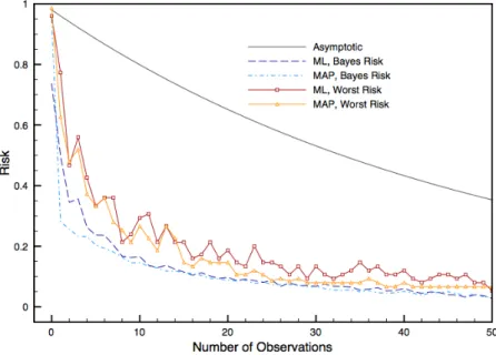
γ= 0.2 . . . 48 3 Empirical and asymptotic worst risk trend forγ= 0.1and
γ= 0.2 . . . 49 4 Bayes and worst risks trend for different reputation
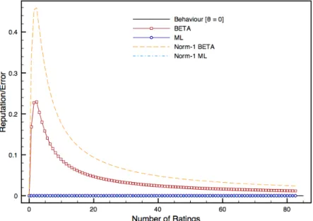
func-tions . . . 50 5 Networked Trust Infrastructure . . . 56 6 Reputation and error trends for parties with behaviourθ=
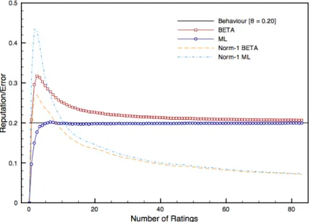
0and no initial ratings assigned . . . 66 7 Reputation and error trends for parties with behaviourθ=
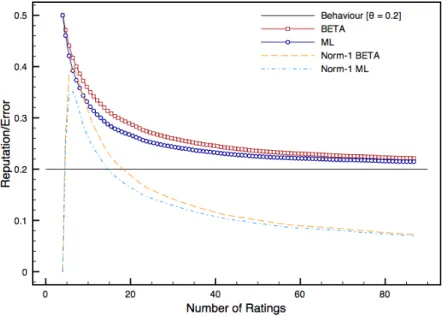
0.20and no initial ratings assigned . . . 67 8 Reputation and error trends for parties with behaviourθ=
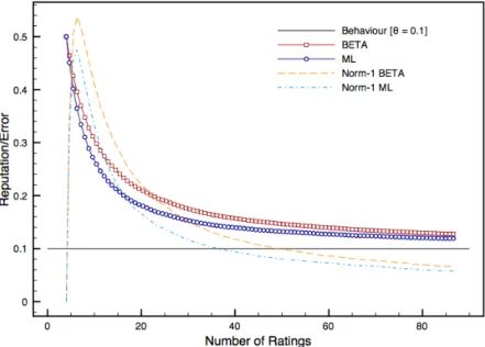
0.10and4initial ratings fixing initial reputation score to0.5 68 9 Reputation and error trends for parties with behaviourθ=
0.20and4initial ratings fixing initial reputation score to0.5 69 10 General infrastructure of a reputation system . . . 76 11 NEVER architecture and workflow . . . 77 12 Trend of parties’ reputation . . . 89 13 Trend of single party’s reputation respect to the reputation
models configured . . . 91 14 Trend of aggregated parties’ reputation, Group 3 . . . 92
15 Risk trend for a single reputation model . . . 93 16 Reputation and error trends for parties with behaviourθ=
0.10and no initial ratings assigned . . . 102 17 Reputation and error trends for parties with behaviourθ=
0.25and no initial ratings assigned . . . 103 18 Reputation and error trends for parties with behaviourθ=
0.30and no initial ratings assigned . . . 103 19 Reputation and error trends for parties with behaviourθ=
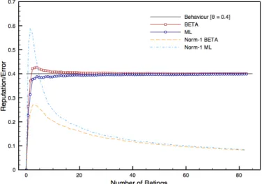
0.40and no initial ratings assigned . . . 104 20 Reputation and error trends for parties with behaviourθ=
0.50and no initial ratings assigned . . . 104 21 Reputation and error trends for parties with behaviourθ=
0.60and no initial ratings assigned . . . 105 22 Reputation and error trends for parties with behaviourθ=
0.70and no initial ratings assigned . . . 105 23 Reputation and error trends for parties with behaviourθ=
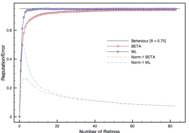
0.75and no initial ratings assigned . . . 106 24 Reputation and error trends for parties with behaviourθ=
0.80and no initial ratings assigned . . . 106 25 Reputation and error trends for parties with behaviourθ=
0.90and no initial ratings assigned . . . 107 26 Reputation and error trends for parties with behaviourθ=
1and no initial ratings assigned . . . 107 27 Reputation and error trends for parties with behaviourθ=
0and4initial ratings, which fix parties’ initial reputation score to0.5 . . . 108 28 Reputation and error trends for parties with behaviour
θ= 0.25and4initial ratings, which fix parties’ initial rep-utation score to0.5 . . . 109 29 Reputation and error trends for parties with behaviour
θ= 0.30and4initial ratings, which fix parties’ initial rep-utation score to0.5 . . . 109
30 Reputation and error trends for parties with behaviour θ= 0.40and4initial ratings, which fix parties’ initial
rep-utation score to0.5 . . . 110
31 Reputation and error trends for parties with behaviour θ= 0.50and4initial ratings, which fix parties’ initial rep-utation score to0.5 . . . 110
32 Reputation and error trends for parties with behaviour θ= 0.60and4initial ratings, which fix parties’ initial rep-utation score to0.5 . . . 111
33 Reputation and error trends for parties with behaviour θ= 0.70and4initial ratings, which fix parties’ initial rep-utation score to0.5 . . . 111
34 Reputation and error trends for parties with behaviour θ= 0.75and4initial ratings, which fix parties’ initial rep-utation score to0.5 . . . 112
35 Reputation and error trends for parties with behaviour θ= 0.80and4initial ratings, which fix parties’ initial rep-utation score to0.5 . . . 112
36 Reputation and error trends for parties with behaviour θ= 0.90and4initial ratings, which fix parties’ initial rep-utation score to0.5 . . . 113
37 Reputation and error trends for parties with behaviourθ= 1and4initial ratings, which fix parties’ initial reputation score to0.5 . . . 113
38 Trend of aggregated parties’ reputation, Group 1 . . . 115
39 Trend of aggregated parties’ reputation, Group 2 . . . 116
40 Trend of aggregated parties’ reputation, Group 4 . . . 116 41 Trend of a single party’s reputation, whose behaviour is
θ= 0.95, with respect to the reputation models configured 117 42 Trend of a single party’s reputation, whose behaviour is
θ= 0.7, with respect to the reputation models configured . 118 43 Trend of a single party’s reputation, whose behaviour is
44 Trend of a single party’s reputation, whose behaviour is θ= 0.05, with respect to the reputation models configured 119 45 Trend of a single party’s reputation, whose behaviour is
θ= 0.3, with respect to the reputation models configured . 119
46 Risk trend for a single reputation model . . . 120
47 Risk trend for a single reputation model . . . 121
48 Risk trend for a single reputation model . . . 121
49 Risk trend for a single reputation model . . . 122
List of Tables
1 KLAIMsyntax . . . 21 2 Satisfaction probability for party’s behaviourθ = 1and
timet= 50 . . . 70 3 Satisfaction probability for party’s behaviourθ = 0.9and
timet= 50 . . . 71 4 Satisfaction probability for party’s behaviour θ = 0.1,
threshold0.35and timet= 20. . . 72 5 Satisfaction probability for party’s behaviour θ = 0.25,
Acknowledgements
The preparation of this thesis is the last step of an experience began on March 2010 at IMT Institute for Advanced Studies, Lucca. In this period I had the chance to meet a lot of people and to have with them interesting discussions.
First of all I must thank Prof. Rocco De Nicola, my super-visor, for his constant support and the useful advices. The same shall be said about Prof. Michele Boreale and Francesco Tiezzi my co-supervisors, with whom I had the pleasure to work. Many other people shall be thanked, Prof. Hanne Riis Nielson and Prof. Flemming Nielson, who hosted me for few months in their research group at Technical University of Denmark. With them and their collaborator I had the op-portunity to have useful and interesting discussions that have been fruitful for my research. Hern´an Melgratti, who hosted me at the Computer Science Department of the Univeristy of Buenos Aires, for his useful suggestions.
A special thanks goes to my family, that has constantly sup-ported me.
Declaration
Part of the material presented in this thesis has been pre-viously published in some co-authored papers. In particu-lar, Chapter 3 is based on [BC13], a joint work with Michele Boreale. Chapters 4 and 5 are instead based on [CDT13b] and [CDT13a], both co-authored by Rocco De Nicola and Francesco Tiezzi.
Vita
May 4, 1983 Born, Viterbo, Italy
May, 2006 Bachelor Degree in Computer Science
La Sapienza, University of Roma, Italy September, 2007 - February, 2008 Exchange Student, Erasmus Programme
KTH Royal Institute of Technology, Stockholm, Sweden
December, 2008 Bachelor Degree in Computer Science
La Sapienza, University of Roma, Italy January, 2009 - March, 2010 Software System Designer
CASPUR, Roma, Italy
March 2010 PhD Student,
IMT Lucca, Italy. March, 2012 - July 2012 Visiting Research Period
DTU Technical University of Denmark Kongens Lyngby, Denmark
November, 2013 - December, 2013 Visiting Research Period University of Buenos Aires, Buenos Aires, Argentina
Publications
1. M. Boreale and A. Celestini, “Asymptotic Risk Analysis for Trust and Rep-utation Systems”, inSOFSEM 2013: Theory and Practice of Computer Sci-ence, Lecture Notes in Computer Science Volume 7741, 2013, pp 169-181, Springer Berlin Heidelberg.
2. A. Celestini, R. De Nicola, and F. Tiezzi, “Specifying and Analysing Rep-utation Systems with a Coordination Language”, in Proceedings of 28th Annual ACM Symposium on Applied Computing (SAC), ACM press, 2013, pp 1363-1368.
3. A. Celestini, R. De Nicola, and F. Tiezzi, “Network-aware Evaluation Envi-ronment for Reputation Systems”, inTrust Management VII – 7th IFIP WG 11.11 International Conference, IFIPTM, 2013.
Presentations
Conference talks:
1. “Specifying and Analysing Reputation Systems with a Coordination Lan-guage”,28th Symposium On Applied Computing, Coimbra, Portugal, March, 2013.
2. “Asymptotic Risk Analysis for Trust and Reputation Systems”, 39th In-ternational Conference on Current Trends in Theory and Practice of Computer Science, ˇSpindler ˚uv Ml ´yn, Czech Republic, January, 2013.
Other talks:
3. “Analysis for Trust and Reputation Systems”,CINA Kick-off Meeting, Pisa, Italy, February, 2013.
4. “Asymptotic Risk Analysis for Trust and Reputation Systems”, University of Buenos Aires, Buenos Aires, Argentina, December, 2012.
5. “A Framework for the Analysis of Trust and Reputation Systems”, 16th MT-LAB Workshop, DTU Technical University of Denmark, Kongens Lyn-gby, Denmark, April, 2012.
6. “A Framework for Network-aware Evaluations of Reputation Systems”, DTU Technical University of Denmark, Kongens Lyngby, Denmark, March, 2012.
Chapter 1
Introduction
The concept of trust is an integrative component of human society. In our daily activities we establish trust-based interactions with others in several contexts. As an example of these interactions we take here the sale of goods. Both in the case of real or virtual markets, in sales we have two parties, the seller and the buyer, each one with different goals. The seller has to trust the buyer, which means that the buyer will pay, that the payment method will be valid, etc. The buyer has to trust the seller, which means that the seller will send the goods by the time stated, that the quality of the goods will be the one stated, etc. Living in a social world, becoming smaller due to networking technologies, interactions are unavoidable, in everyday lives we are constantly interacting with something or someone. In such interactions we always deal with the issue of how to evaluate others’ trustworthiness.
In this thesis our aim is more specific, we are interested in trust interactions taking place among parties in distributed systems. Such parties can be human beings using devices or just devices communi-cating and executing code. In computer science, there are many def-initions and models for trust management (see, e.g., those reported in [BFIK99; ZM00; JIB07; SS05]). Such issue is usually tackled in the field of computer security and, on the basis of the mechanism used for trust management, we talk ofhardorsoftsecurity mechanisms [RJ96].
Trust and reputation systems are a specific approach to trust man-agement. Such systems are used as decision support tools for different applications in several contexts. In recent years, we have seen an increas-ing use of them in different areas of ICT, from e-commerce to different forms of open computer networking. This phenomenon is likely to con-tinue, due to the success of networked applications (like social networks or other Web 2.0 technologies) and to the need, in such environments, of instruments to build up relationships of trust among interacting parties. Probably, the best known applications making use of trust and repu-tation systems are those related to e-commerce: well-known examples in this context are the auction site eBay, the online shop Amazon, and soft-ware application stores, like Google Play and Apple App Store. How-ever, trust management systems are used in many other contexts and applications, where huge amount of data related to reputations of peers are usually available, such as ad-hoc networks [NCL07], P2P networks [XL04; WV03] and sensor networks [BXEK07]. Parties, which are will-ing to interact in these environments, are likely to be disconnected from their preferred security infrastructures and/or have no trusted informa-tion about their partners. Thus, they have to rely on other techniques to build up relationships of trust among each other.
The idea at the base of trust and reputation systems is to let their users, theraters, rate the services providers, theratees, after each interac-tion. For instance, rating values could refer to the quality of a service, or to the success of the interaction. Figure 1 graphically depicts such generic scenario where a trust and reputation system is in use: parties active in the system freely interact (Figure 1 (a)) and rate each other after each in-teraction (Figure 1 (b)). Then, other users or the parties themselves may use aggregate ratings to compute reputation scores for a given party. The computedreputationscores are a collective measure of parties’ trustwor-thiness and are used to drive parties’ interactions, i.e. a party selects the party to interact with on the basis of its reputation score. This approach to trust management is referred to ascomputational trust. In computa-tional trust parties’ trustworthiness is evaluated on the basis of parties’ past behaviour, whereascredential-basedapproaches [EFL+99; NT94] rely
(a) Interactions between parties ratee rater rater ratee rater ratee ratee rater (b) Rating release
Figure 1:A generic scenario in which a reputation system is in use
on access control policies and/or use of certificates for evaluating parties’ trustworthiness.
In the following we briefly present the two categories of trust man-agement approaches, namely credential-based and computational trust.
1.1
Credential-based Trust
Credential-based approaches are based mainly on two concepts: authen-ticationandauthorization. In such approaches the aim is to authenticate parties and then check if parties are allowed to perform the actions they are trying to carry out. Indeed, we can say that parties’ trustworthiness
is evaluated on the basis of parties’ credentials. The assumptions are that all parties interacting in the systems can be authenticated and that, for each of them, there exists a policy stating which actions it is autho-rized to perform. Two issues immediately arise, first all parties have to be known in advance in order to be authenticated. Second, a policy rule for each of them should be set.
In distributed systems the first issue, about parties authentication, is usually addressed through public key cryptography. In public key cryp-tography each party in the system is assumed to own a key pair<public key, private key>. The private key is known only by the owner of the pair, while the public key is known by everyone. Below, we present the general idea at the base of public key authentication protocols. If party Awants to authenticate partyB, assumingAknowsB’s public key, the basic protocol run by the two parties works as follows: let< eB, dB >
the key pair ofBandra random number chosen byA. PartyAsendsr encrypted withB’s public keyeBtoB. PartyBproves it knowsdB, that
is its identity, by decrypting the message and sending backrtoA. In a system with thousand of parties the question is how to securely manage thousand of public keys. Such issue is usually addressed trough the use of a public key infrastructure (PKI) [KPS02; TW10]. The basic compo-nents of a PKI are: certificates, a repository for retrieving certificates, a method of revoking certificates, and a method of evaluating a chain of certificates.
For the second issue, concerning policy rules stating which actions parties can perform, there exist several access control models enabling to control access to data, resources and systems [NIST09]. The oldest and most basic form of access control are the Access Control Lists (ACLs). An ACL states for each resource in the system which are the parties that can access it and which actions they can perform on it. In addition to ACLs there are several others models, such as Role-based Access Con-trol (RBAC), Attribute Based Access ConCon-trol (ABAC) and Policy-Based Access Control (PBAC). All these models try to address shortfalls of the others and are tailored for specific environments, thus the choice of the access control model should be made on the basis of systems’ features.
Below, as reference standards in traditional trust, we briefly remind Kerberos, X.509, PGP, SSL/TLS and XACML.
Kerberos. Kerberos is a secret key based service for providing authen-tication in a network, where the access to remote resources is granted to users after authentication. In Kerberos, user’s workstation performs the authentication protocol on user’s behalf and the network itself is as-sumed to be insecure. Two servers are used to manage authentication and resource access, the Authentication Sever and the Ticket-Granting Server. We refer the reader to [KPS02; TW10; NT94] for an extensive discussion of Kerberos.
X.509 and PGP. The X.509 and PGP standards are two well-known cer-tificate systems, they mainly differ for the way public keys are certified and how certificate chains are verified. The standard X.509 assumes ex-istence of entities called certification authorities, which release certifi-cates and sign them. Instead, with PGP, each user generates its pair of keys and decides which keys to trust. New trusted keys are got directly from new users or introduced by trusted users. We refer the reader to [KPS02; TW10] for an extensive discussion of X.509 and PGP.
SSL/TLS. The SSL/TLS standard is used to establish secure network connections. It is broadly used in web applications, mainly for e-commerce transactions. Indeed, the use of HTTP over SSL, called HTTPS, is the most common application of the SSL/TLS protocol. We refer the reader to [KPS02; TW10] for an extensive discussion of the SS-L/TLS protocol.
XACML. The eXtensible Access Control Markup Language (XACML) is a general-purpose access control policy language implemented in XML. XACML was developed to specify access control policy in a machine-readable format. With XACML it is possible to implement ABAC systems or RBAC systems as a specialization of ABAC systems. XACML is also used in PBAC systems, in such systems policies creation
can be complicated and XACML is a useful means for creating, specify-ing, and enforcing effective access control policies. We refer the reader to [XACML; NIST09] for an extensive discussion of XACML and access control models.
However, credential-based approaches are not well suited for open environments, where the sets of parties and resources dynamically change in time.
1.2
Computational Trust
In computational trust approaches, parties’ trustworthiness is evaluated on the basis of the parties’ past behaviour. The assumption at the base of such approaches is to have a distributed system where several parties freely interact. After each interaction,ratersrate the services providers, then the rater itself, or other parties, may use such ratings to compute reputation scores for a given party. Party’s reputation is the synthetic pa-rameter estimating the party’s behaviour and is used to evaluate parties trustworthiness.
Depending on the computational trust model in use, the ratings re-leased by parties can assume values in different domains. There are models in which each interaction can be evaluated using just two values, representing the success and the failure of the interaction [JI02; DA04]. Another possibility is using rating values in an interval of n values, with each rating representing the quality of the service provided [JH07; DA04]. There are also models where instead of numerical values, at-tributes are used to rate parties, e.g. in [ARH00] the following atat-tributes are used: very trustworthy, trustworthy, untrustworthy, very untrust-worthy.
Trust and reputation are often used as synonyms in the literature. In our work we comply with the distinction made in [JIB07]. According to [JIB07], trust is a subjective perception of reliability of a party, mainly derived from private knowledge and/or belief (e.g., direct interactions with the party). Instead, reputation is an objective measure of partys
trustworthiness derived from referrals or ratings provided by other par-ties. Parties can trust other parties despite their reputation values, this is due to the subjectivity property of trust. Indeed reputation systems are used as decision support tools where reputation values are used to drive parties interactions.
More specifically, in our work we focus on probabilistic trust [SKN07; KNS08; MMH02; TPJL06; JI02], which represents a specific approach to computational trust. The basic postulate of probabilistic trust is that the behaviour of each party can be modeled as a probability distribution, drawn from a given family, over a certain set of interaction outcomes (success/failure being the simplest case). In this approach the task of computing reputation scores reduces to inferring the true distribution’s parameters for a given party. The information about party’s past be-haviour is used for such inference, i.e. rating values are treated as statis-tical data in the inference process.
1.3
Contribution
Due to the widespread use of reputation systems, research work on them is intensifying and several models have been proposed [JIB07; LLYY09; SS05; MGM06]. Thus, once a reputation system has to be designed sev-eral choices have to be made at different levels of the development pro-cess, before its deployment in a network environment. This calls for a methodology for the analysis and the evaluation of trust and reputation systems that can help researchers and developers in studying, designing and implementing such systems. We address this challenge by propos-ing different kinds of theoretical and software frameworks and tools that, in our opinion, can support the development of trust and reputation sys-tems.
The main contributions of our work can be summarized as follows: 1. Theoretical Framework: a general framework based on Bayesian
decision theory for the theoretical assessment of trust and reputa-tion models.
2. Analysis Methodology: a methodology for analysing reputation systems based on a coordination language.
3. Software Tool:a software environment for network-aware evalua-tion of reputaevalua-tion systems and their rapid prototyping.
Theoretical Framework. Whenever existing or new reputation models have to be analysed, a theoretical framework for the assessment of such models is needed. In this phase it is interesting to study the models on the basis of a small set of simple parameters, such as quantity of available information and decision strategies, while abstracting from implementa-tion and deployment details. To this aim, we propose a general frame-work based on Bayesian decision theory for the assessment of trust and reputation systems. Within our theoretical framework we study how to quantify theconfidencein the decisions calculated by the system. We anal-yse how this confidence is related to parameters as decision strategy and number of available ratings. We analyse if there are optimal strategies that maximize confidence when additional information becomes avail-able.
In our analysis, we study the behaviour of trust and reputation sys-tems by relying on the concept oflossfunction; a loss function evaluates the consequences of possible decisions taken by the system associating a loss to each decision. We quantify theconfidencein the decisions calcu-lated by trust and reputation systems in terms ofriskquantities based on
expected (also known as bayes)andworst-caseloss. We study the behaviour of these quantities with respect to the available information, that is the number of available rating values and the decision strategy, in the case of independent and identically distributed observations. We show that there are optimal strategies that maximize confidence as more and more information becomes available. Finally, we study an extention of our framework to a class of rating mechanisms where each rater is charac-terised by a (unobservable, possibly malicious) bias. This can lead the rater to under- or over-evaluate its interactions with the ratees.
Analysis Methodology. Concerning the integration of reputation sys-tems with end-user applications, a methodology for tuning trust and rep-utation models in order to fit to the characteristics of the given network environment is needed. In particular, it is interesting to study whether in the phase of models tuning, the features of the original models are kept. We address such issues by proposing a verification methodology based on the use of the coordination language KLAIM[BBD+03; DFP98] and related analysis tools [DKL+07; Lor10]. Such approach enables ver-ification of reputation system specver-ifications. Specifically, it is possible to check whether trust and reputation models meet the expected behaviour, how parties’ initials reputations affect the models and how parties’ be-haviours affect their reputations. In our study, we first define a paramet-ric KLAIMspecification of a reputation system that can be instantiated with different reputation models. Then, we consider a stochastic spec-ification obtained by considering actions with random (exponentially distributed) duration. The resulting specification allows us to perform quantitative analysis of estimation properties of the considered system.
Software Tool. The last issue we address is related to implementation, i.e. to the phase when reputation systems have to be deployed and tested in real network environments. At this stage, real-word implementation details of trust and reputation systems and of the network environment where they have to be deployed have to be taken into account in the eval-uation. We have developed a software tool (NEVER) for network-aware evaluation of reputation systems and for their rapid prototyping through experiments performed according to user-specified parameters. On the one hand, NEVER provides a framework for rapidly developing Java-based implementations of reputation system models and for easily con-figuring different networked execution environments on top of which the reputation systems will run. On the other hand, NEVER can be used for automatically performing experiments on the reputation system im-plementations according to user-specified parameters; this enables the study of their behaviour while executing on given network infrastruc-tures.
Overall our contribution addresses issues related to the study, the de-sign and the implementation of trust and reputation systems. Indeed, we provide theoretical and software tools for the analysis and evaluation of trust and reputation systems, at different stages of their development.
1.4
Structure of the thesis
The rest of the thesis is organized as follows. In Chapter 2 we briefly in-troduce the technical concepts used throughout the thesis. We first recall some basic notions of Probability Theory, Information Theory and dis-cuss some relationships between Information Theory and Statistics. We describe the basic concepts of Bayesian Decision Theory and, introduce the coordination language KLAIMand related analysis tools. Then, we give an overview of probabilistic trust approaches by describing some of the models proposed in the literature. Finally, we show some cases of reputation systems that are successfully used in real applications.
In Chapter 3 we present our general framework, based on Bayesian decision theory, for the assessment of trust and reputation models. We introduce the framework and discuss our results on the analysis of such systems. We close the chapter by presenting an extention of the frame-work for different data models, with rating values given in different ways.
In Chapter 4 we introduce a verification approach for reputation sys-tems that is based on the use of the coordination language KLAIMand related analysis tools. We define a parametric KLAIM specification of a reputation system that can be instantiated with different reputation models. Then, we consider stochastic specifications enabling quantita-tive analysis of properties of the considered system. Finally, we present verification results on some reputation systems.
In Chapter 5 we present NEVER, a software tool for network-aware evaluation of reputation systems and their rapid prototyping. The NEVER evaluation of reputation systems is carried out through exper-iments performed according to user-specified parameters. In such ex-periments the networked execution environment is explicitly taken into
account. We close the chapter by presenting some evaluation results ob-tained with our tool.
In Chapter 6 we comment on the research results presented in the the-sis by also comparing them with more closely related work. We summa-rize the main contributions and propose possible directions for further research.
Chapter 2
Preliminaries
In this chapter we briefly introduce the technical concepts used in the rest of the thesis. In Section 2.1 we recall some basic notions of Probabil-ity Theory. In Section 2.2 we introduce Information Theory and Statistics and show their relationship. In Section 2.3 we describe the basic concepts of Bayesian Decision Theory and in Section 2.4 we introduce the coordi-nation language KLAIMand related analysis tools. Finally, in Section 2.5 we give an overview of probabilistic trust approaches and in Section 2.6 we describe the operation of some reputation systems used in real appli-cations.
2.1
Probability Theory
Probability theory is technically a branch of measure theory, it reasons about chance, uncertainty, likelihood of phenomena. In this section, we first introduce few notions of measure theory then we recall some basic notions of probability theory. We refer the reader to [Wil91; Sti99; GS01; Kal02] for an extensive presentation of these topics.
Below we provide the definitions of σ-f ield, measure space, measur-able setandmeasureto then introduce some basic notions of probability theory.
Fof subsets ofΩsatisfying the following conditions: (a) ∅ ∈ F,
(b) A∈ F ⇒ Ac∈ F, whereAcdenotes the complement set,
(c) A1, A2, ..., An∈ F with n∈N ⇒ SnAn ∈ F
The smallestσ-f ieldassociated with Ωis the collection F = {∅,Ω}
and the largest one is thepower setofΩ, written2Ω. Ameasurable setis a pair(Ω,F), whereΩis a set andFis aσ-f ieldonΩ.
Definition 2.1.2 Let(Ω,F)a measurable set, ameasureon(Ω,F)is a func-tionµ:F →[0,∞)such that:
(a) µ(∅) = 0, (b) µ(A) = P
nµ(An), whereAn(n∈ N)is a sequence of pairwise
dis-joint sets inFwith unionA=S
nAn.
The triple(Ω,F, µ)is then called ameasure space.
Aprobability measure Pon (Ω,F)is a measure such that P(Ω) = 1.
The triple(Ω,F,P)is calledprobability spaceand the setΩis calledsample space. A pointωofΩis called asample pointoroutcome. The collectionF
is calledfamily of eventsand aneventis an element ofF. If A and B are two events andP(B) > 0, then the conditional probabilitythat A occurs
given that B occurs is defined as
P(A|B) =P(A∩B)
P(B) (2.1)
We denote with P(A|B) the conditional probability and we read “the
probability of A given (or conditioned on) B”. It is not always the case that the occurrence of an eventB changes the probability that an-other eventAoccurs. If the conditional probabilityP(A|B)remains
un-changed, i.e. P(A|B) = P(A), then we say thatAandB areindependent.
More formally, eventsAandBare called independent if
Experimental outcomes are not always numerical, but it is often bet-ter to work with numbers than with outcomes in the original sample space. We can assign a number to any outcomeω∈Ωusingrandom vari-ables. A random variable is a real-valued functionX : Ω →Rsuch that
{ω ∈ Ω : X(ω) ≤ x} ∈ F for eachx ∈ R. We can think of a random
variable just as a function mappingΩinR. We denote random variables
with upper-case letters, such asX, Y, Zand their possible numerical val-ues with lower-case letters, such asx, y, z. A distribution function is as-sociated with every random variable. Adistribution functionof a random variableX is a functionF:R→[0,1]such thatF(x) =P(X≤x), where
{X ≤x}denotes the event{ω∈Ω :X(ω)≤x}. We denote withFXthe
distribution function of the random variableX.
A random variableX is calleddiscreteif it takes values only in some countable subsetXofR. We denote with calligraphic lettersX,Y,Z
pos-sible subsets ofR. Theprobability mass functionofXisp:R→[0,1]such
thatp(x) =P(X =x). A random variableXis calledcontinuousif it takes
values in some uncountable subsetX ofRand if its distribution function
can be expressed asF(x) = Rx
−∞p(u)du, for some integrable function p(x)called theprobability density functionofX.
LetX be a discrete random variable, its expected value, denoted by
E[X], is defined as
E[X] =X
x
xP(X =x) (2.3)
Notation: LetX be a random variable taking values inX, we say that X is distributed according to a probability distributionp(·)if for each x ∈ X, P(X = x) = p(x), and we write X ∼ p(·). We will use the
term probability distribution both denoting probability mass function and probability density function, the use will be clear by the context. Thesupport ofp(·)is defined as supp(p) = {x∈ X : p(x) > 0}. We let pn(·)denote then-th extension ofp(·), defined aspn(xn) = Qn
i=1p(xi),
wherexn = (x1, x2, ..., x
n); this is in turn a probability distribution on
the setXn. For anyA⊆ X we letp(A)denoteP
x∈Ap(x). WhenA⊆ X n
2.2
Information Theory and Statistics
Information theory reasons about quantification of information. The fun-damental measure of information is calledentropy, which quantifies the self-information of a random variable, i.e. the uncertainty involved in predicting its value. We refer the reader to [CT06] for an extensive pre-sentation of the topic.
LetXbe a discrete random variable taking value in setXand proba-bility mass functionp(x) = P(X =x), x ∈ X. TheentropyH(X)ofX is defined as
H(X) =−X
x∈X
p(x) logp(x) (2.4)
Thelogis to the base2and entropy is expressed in bits. The entropy of a random variable measures the average amount of information required to describe the random variable.
Given two distributionspandqon the same set X, the relative en-tropy is a measure of the distance between these two distributions. The
relative entropy, orKullback-Leibler distanceD(p||q), between two probabil-ity mass functionsp(x)andq(x)is defined as
D(pkq) =X
x∈X
p(x) logp(x)
q(x) (2.5)
with the convention that0 log0
0= 0,0 log 0
q = 0andplog p
0 =∞. It can be shown that the Kullback-Leibler distance (KL-dis) is always nonnegative and is0if and only ifp=q. D(pk q)it is not a true distance since it is not symmetric and does not satisfy the triangle inequality. The KL-dis D(pkq)is a measure of the inefficiency of assuming that a distribution isqwhen the true distribution it is actuallyp.
We now introduce some concepts at the basis of the relationship be-tween information theory and statistics. We then consider the problem of hypothesis-testing and which is the best possible error exponents for such tests. Letxn=x1, ..., x
na sequence ofnelements from a setX, with
n >0, anda ∈ X. We denote withN(a, xn)the number of occurrences
txn, and is the relative proportion of occurrences of each element
txn(a) =
N(a, xn)
n for alla∈ X. (2.6)
Thetypetxn is a probability distribution onX. LetPn denote the set of
types with denominatorn, it is possible to show that the number of types is at most polynomial inn. Since the number of sequences is exponential inn, it follows that at least one type has exponentially many sequences in its type class.
LetΘbe a set of parameters: we let{p(·|θ)}θ∈Θdenote a parametrized family of probability distributions. When convenient, we shall denote a member of this family,p(·|θ), as justpθ. Given a sequencexn that is a
realization ofnindependent and identically distributed (i.i.d.) random variablesXn =X
1, ..., Xn, withXi∼p(·|θ), a standard problem is to
de-cide which of the distributionsp(·|θ)generated the data. This is a general hypothesis-testing problem, where the distributionsp(·|θ),θ∈Θ, are the hypotheses: the classical, binary formulation is given for|Θ|= 2. We rep-resent the decision-making process by a guessing functiong : Xn →Θ
and we define the error probability for an hypothesisθas follows. For n ≥ 1and each θ, letA(θn) = g−1(θ) ⊆ Xn be the acceptance regionfor
hypothesisθ (relatively tog) and letAθ(n)c the complement set ofA(θn). Then the probability of error forθis
Pθ(g)(n) =p(A(θn)c). (2.7) In a Bayesian framework, an a priori probabilityπ(θ)is assigned to each hypothesis, and the overall error probability is defined as the aver-age, assumingΘis discrete:
Pe(g)(n) =
X
θ
π(θ)Pθ(g)(n). (2.8)
It is well-known (see, e.g., [CT06]) that optimal strategies, i.e. strate-giesgminimizing the error probabilityPe(g)(n), are obtained wheng
formal definition of this criterion). In this case, providedp(·|θ)6=p(·|θ0) forθ6=θ0, it holds that asn→+∞,Pe(g)(n)→0. What is also important,
though, is to characterizehow fastthe probability of error approaches0. Intuitively, we want to be able to determine an exponentρ≥0such that, for largen,Pe(g)(n)≈2−nρ.
To this purpose, we introduce the notion of rate for a generic non-negative real-valued functionf.
Definition 2.2.1 (Rate) Letf :N→R+be a nonnegative function. Assume
γ = limn→∞f(n)exists. Then, provided the following limit exists, we define
the following nonnegative quantity:
rate(f) = lim
n→∞− 1
nlog|f(n)−γ|.
This is also written as|f(n)−γ|= 2. −nρ, whereρ= rate(f).
Intuitively,rate(f) =ρmeans that, for largen,|f(n)−γ| ≈2−nρ. Note
that we do allowrate(f) = +∞, a case that arises for example whenf(n) is a constant function.
The rate of decrease ofPe(g)(n)is given byChernoff Information. Given
two probability distributionsp,qonX, we let their Chernoff Information be C(p, q) =− min 0≤λ≤1log( X x∈supp(p)∩supp(q) pλ(x)q1−λ(x)) (2.9)
where we stipulate thatC(p, q) = +∞ifsupp(p)∩supp(q) = ∅. Here C(p, q)can be thought of as a sort of distance betweenpandq: the more pandq are far apart, the less observations are needed to discriminate between them. Assume we are in the binary case,Θ = {θ1, θ2}and let pi = p(·|θi)fori = 1,2. Then a well-known result gives us the rate of
convergence for the probability of error, with the proviso thatπ(θ1)>0 and π(θ2) > 0 (cf. [CT06]): P
(g)
e (n) = 2. −nC(p1,p2) (here we stipulate
2−∞ = 0). Note that this rate does not depend on the prior distribution π(·)on{θ1, θ2}, but only on the probability distributionsp1andp2. This result extends to the case|Θ|<+∞, it is enough to replaceC(p1, p2)by minθ6=θ0C(p(·|θ), p(·|θ0)), thus (see [LJ97; BPP11]):
Pe(g)(n)= 2. −nminθ6=θ0C(p(·|θ),p(·|θ
0))
with the understanding that, in themin,π(θ)>0andπ(θ0)>0.
2.3
Bayesian Decision Theory
Statistical decision theory concerns with the process of making decisions in presence of statistical knowledge. The general assumption is that the uncertainties involved in the decision process can be expressed as un-known numerical values,θ. Such values are calledworld statesor param-eters; we denote withΘthe set of all possible parameters. The statisti-cal knowledge is used to obtain information about the parameters. In a Bayesian setting an other type of information is particularly relevant, theprior information. Such information comes from other source than the statistical investigation.
The main components of bayesian decision theory are three:
1. an a prior distributionπ(·)over the world statesΘ. Such distribu-tionπ(·)represents a prior information about the world states, in addition to sample information.
2. an observational model p(·|·), that represents how data are gen-erated in the world. The value p(o|θ)denotes the probability of observingo∈ Owhen the world state isθ∈Θ.
3. a loss functionL(·,·) : Θ× D → R+, whereDdenote the decision set. The loss functionL(θ, d)gives the loss incurred when a deci-siond∈ Dis made and the state of the world turns out to beθ. Determined the components of the model, the decision making process consists of making a decisiondon the basis of a sequence of observations on =o
1, ..., on, withn > 0andon ∈ On. In bayesian decision theory the
decision making process is formalized via decision functions. For anyn, a decision function is a functiong:On→ D.
The choice of an optimal decision relay on the concept of loss, that is computed through loss functions. Several standard types of loss can be considered, we report below some example of them. In Chapter 3 we use a Bayesian decision theory framework for our analysis of trust and
reputation systems. For an extensive presentation of Bayesian decision theory we refer the reader to [Ber85; Rob07].
2.3.1
Loss Functions
Loss functions evaluate the consequences of possible decisions, by asso-ciating a loss to each of them. Often it is not straightforward how this evaluation should be done, it depends on the system features. Below we list a few standard definitions of loss functions.
Linear Loss The loss L(θ, d) =
(
k0(θ−d) if (θ−d)≥0, k1(d−θ) if (θ−d)<0
is calledlinear loss. The constantsk0andk1are usually different, they re-flect the importance of underestimation and overestimation, respectively. When the two constants are equal the loss is equivalent toL(θ, d) =
|θ−d|, which is calledabsolute loss. 0-1 Loss The loss
L(θ, di) =
(
0 if θ∈Θi,
1 if θ∈Θj (j6=i)
is called0-1 loss. In this case two decisions are possible, i.e.D={d0, d1}, and the loss associated to each decision can be only0 or1. It is0 if a correct decision is made and 1 otherwise, e.g. d0is correct ifθ∈Θ0and d1is correct ifθ∈Θ1. This loss is mainly used in the case of two-actions decision problems, e.g. hypothesis testing.
Squared-Error Loss The loss function L(θ, d) = (θ − d)2 is called
squared-error loss. This loss function penalizes large errors. Anyway, this penalization could be considered too severe in some systems.
2.4
The KLAIM
Coordination Language and
Re-lated Tools
In this section we informally present KLAIM[BBD+03; DFP98], a coor-dination language specifically designed for modelling mobile and dis-tributed applications and their interactions, which run in a network en-vironment. Then, we introduce the KLAIM’s stochastic extension STO
K-LAIM[DKL+06a; DLM05; DKL+07], the stochastic logic M
OSL [DKL+07; DKL+06b] and the analysis tool SAM [DKL+07; Lor10]. Finally, we in-troduce KLAVA[BDP02], a Java library implementing the run-time
sup-port for KLAIMactions.
2.4.1
K
LAIMIn our presentation of the KLAIM language we consider a version of KLAIMenriched with standard control flow constructs (i.e., assignment, if-then-else, sequence, etc.). Such constructs were not included in the original presentation of the language [DFP98], however they can be eas-ily rendered in KLAIM(by resorting, e.g., to choice, fresh names and re-cursion in the usual way) and are directly supported by related tools.
The syntax we use is reported in Table 1, wheres,s0,. . . range over
locality names (i.e., network addresses); self, l, l0,. . . range overlocality variables(i.e., aliases for addresses);`,`0,. . . range over locality names and variables; x, y,. . . range over value variables; X, Y,. . . range over process variables;e,e0,. . . range overexpressions1;A,B,. . . range overprocess
identi-fiers2. We assume that the set of variables (i.e., locality, value and process
variables), the set of values (locality names and basic values) and the set of process identifiers are countable and pairwise disjoint.
KLAIMnetsare finite plain collections of nodes wherecomponents, i.e.
1The precise syntax of expressions is not specified here. Suffice it to say that expressions
contain basic values (booleans, integers, strings, floats, etc.) and variables, and are formed by using the standard operators on basic values, simple data structures (i.e., arrays and lists) and the non-blocking retrieval actionsinpandreadp(explained in the sequel).
2We assume that each process identifierAwith aritynhas a unique definition, visible
from any locality of a net, of the formA(f1, . . . , fn),P, wherefiare pairwise distinct. Notably,piandfjdenote actual and formal parameters, respectively.
(Nets) N ::= 0 s ::ρ C N1kN2 (νs)N (Components) C ::= hti P C1|C2 (Processes) P ::= nil a P1;P2 P1|P2 if(e)then{P}else{Q} fori=ntom{P } while(e){P} A(p1, . . . , pn) (Actions) a ::= in(T)@` read(T)@` out(t)@` eval(P)@` x := e inp(T)@` readp(T)@` rpl(T)→(t)@` newloc(s) (Tuples) t ::= e ` P t1, t2 (Templates) T ::= e ` P !x !l !X T1, T2
Table 1:KLAIMsyntax
processes and data tuples, can be allocated. KLAIMspecifications consist of nets, namely finite plain collections of nodes where components, i.e. processes and data tuples, can be allocated. Nodes are composed by means of the parallel composition operator k . At net level, it is possible to restrict the visibility scope of a namesby using the operator(νs) : in a net of the formN1 k (νs)N2, the effect of the operator is to make s invisible from within the subnetN1.
Nodeshave the forms ::ρ C, wheresis a unique locality nameρis
an allocation environment, andCis a set of hosted components. An al-location environmentprovides a name resolution mechanism by mapping locality variablesl, occurring in the processes hosted in the correspond-ing node, into localities. The distcorrespond-inguished locality variableselfis used by processes to refer to the address of their current hosting node. In the rest of this section, we will use`to range over locality names and vari-ables.
ex-ecuted concurrently either at the same locality or at different localities. They are built up from the processnil, which does nothing, and from basic actions by means of sequential composition ; , parallel composi-tion | , conditional choice if (e)then{ }else{ }, the iterative con-structsfor i = n to m { } and while (e){ }, and process definition A(f1, . . . , fn), .
During their execution, processes perform some basic actions. Ac-tionsin(T)@` andread(T)@`are retrieval actions and permit to with-draw/read data tuples (i.e. sequences of values) from the tuple space hosted at the (possibly remote) locality`: if a matching tuple is found, one is non-deterministically chosen, otherwise the process is blocked. These actions exploit templates as patterns to select tuples in shared tu-ple spaces.Templatesare sequences of actual and formal fields, where the latter are written!x,!l or!X and are used to bind variables to values, locality names or processes, respectively.
Actionsinp(T)@`andreadp(T)@`are non-blocking versions of the retrieval actions: namely, during their execution processes are never blocked. Indeed, if a matching tuple is found,inpand readpact sim-ilarly toinandread, and additionally return the boolean valuetrue; oth-erwise, they return the valuefalseand the executing process does not block. Actionsinp(T)@` and readp(T)@` can be used where either a boolean expression or an action is expected (in the latter case, the re-turned value is simply ignored).
Actionout(t)@`adds the tuple resulting from the evaluation of tuple t(which may contain expressions) to the tuple space of the target node identified by`, while actioneval(P)@`sends the processPfor execution to the (possibly remote) node identified by`. Actionsoutandevalare both non-blocking.
Action rpl(T) → (t)@` atomically replaces a non-deterministically chosen tuple in` matching the template T by the tuple t; if no tuple in`matches T, the action behaves asout(t)@`. Finally, actionnewloc creates new network nodes, while actionx := eassigns the value ofeto x. These latter two actions, differently from all the others, are not indexed with an address because they always act locally.
2.4.2
Stochastic Analysis of KLAIM Specification
In this section we introduce the related analysis tool of KLAIM, that en-ables us to perform quantitative analysis of systems. In general, two main kind of analysis can be performed over systems, quantitative or qualitative analysis. In qualitative analysis we verify that a certain event will or will not occur. In quantitative analysis instead, we verify what is the probability that a certain event will or will not occur. In order to perform such analysis of KLAIM specification, we have to enrich such formalism by enabling the modelling of random phenomena. KLAIM
specifications can be enriched with stochastic aspects, using the KLAIM’s stochastic extension STOKLAIM, while the desired properties of the
con-sidered system can be expressed by using the stochastic logic MOSL. The
properties of interest are then checked against the STOKLAIM specifica-tions by means of the analysis tool SAM. In this section we provide an overview of STOKLAIM, MOSL and SAM.
STOKLAIM
In STOKLAIM[DKL+06a; DLM05; DKL+07], K
LAIM’s processes actions are enriched with a rate. Such rate is the parameter of an exponentially distributed random variable characterising the duration of the execution of an action. In particular, such random variables are governed by a negative exponential distribution. The negative exponential distribution is related to the Poisson distribution. It describe the times between events in a Poisson process, i.e. a process in which events occur continuously at a constant average rateλ; independently of the timet. A real valued random variableXhas anegative exponential distributionwith rateλ >0 if and only if the probability thatX ≤t, witht > 0, i.e. the probability that an event occurs withinttime units, is1−e−λ·t. The expected value
ofX isλ−1, while its variance isλ−2.
The operational semantics of STOKLAIMpermits associating to each specification a Continuous Time Markov Chain (CTMC), one of the most popular models for the evaluation of the performance and dependability of information processing systems. Such CTMC is then used to perform
quantitative analyses of the considered system. The use of the exponen-tial distribution is motivated by the fact that it enjoys convenient prop-erties enabling automated analyses that are not always allowed by other distributions.
MOSL
The desired properties of a system under verification are formalised us-ing the stochastic logic MOSL [DKL+07; DKL+06b]. M
OSL formulae use predicates on the tuples located in the considered STOKLAIMnet to ex-press the reachability of a certain system state, while passing through, or avoiding, other specific intermediate states.
The Mobile Stochastic Logic (MOSL) is an extension of a widely used
temporal logic, CTL [EC82]. MOSL is inspired by (an action-based
version of) CSL [ASSB00; BKH99], a stochastic extension of CTL that, together with qualitative properties, permits specifying time-bounded probabilistic reachability properties. The logic is both action- and state-based. MOSL incorporates some basic features of the Modal Logic for Mobility (MOMO) [DL05], in order to be able to refer to the distributed character of the specified systems. Specificallybasic state formulae are built using a variant of the MOMO consumption (→)and production (←)operators. Intuitively, a consumption formula
A(p1, ..., pn)@`→Φ
holds for a network whenever in the network there exists a process A running at a node, of site `, and the remaining network, namely A(p1, ..., pn)’s context, satisfies Φ. Notice that a process binder!X can
be used instead of process. Similarly formula
hTi@`→Φ
holds whenever a tupletmatchingT is stored in a node of site`, and the remaining network satisfiesΦ. The substitution resulting from pattern-matching is used to evaluateΦ.
A production formula
hti@`←Φ
holds if the network satisfiesΦwhenever tupletis stored in a node of existing site `. In particular, the satisfaction of Φ is checked after the insertion of the tupletin the network.
We can summarise the grammar for basic state formulae as follows:
ℵ::= A(p1, ..., pn)@`→Φ | !X@`→Φ | < T >@`→Φ
| A(p1, ..., pn)@`←Φ | < t >@`←Φ
MOSL distinguishes betweenpathandstateformulae. The basic for-mat ofpath formulaeis the CTL untilformulaΦUΨ. In particular, the logic use an action-based variant of the until operator, parameterised with two action sets: a path satisfiesΦ∆UΩΨwhenever (eventually) a state satisfyingΨ(a Ψ-state) is reached via aΦ-path (i.e., a path com-posed only of Φ-states) and, in addition, while evolving between Φ -states, the performed actions satisfy∆, and theΨ-state is entered via an action satisfyingΩ. Path formulae have also a time constraint. This is done by adding time parametertwhich is either a real number or∞. With time constraint, it is now imposed that aΨ-state should be reached withinttime units. Similarly, a path satisfiesΦ∆U<tΨif the initial state satisfiesΨ(at time 0) or eventually aΨstate will be reached in the path, by timetvia aΦ-path, and, in addition, while evolving betweenΦ-states, actions are performed satisfying∆. Accordingly, the syntax of path for-mulae is:
ϕ::= Φ U<t
∆ Ω Ψ | Φ U
<t
∆ Ψ.
State formulaeare divided in three categories. The first category in-cludes formulae in propositional logic, where the atomic propositions arett and the basic state formulaeℵintroduced previously in this sec-tion. The second category includes statements about the likelihood of paths satisfying a property,P./p(ϕ). Finally the third category includes
formulae for the so-called long-run properties,S./p(ϕ). In general, a
bit more precise about the probabilistic path properties. Letϕbe a prop-erty imposed on paths. Statessatisfies the propertyP./p(ϕ)whenever
the total probability mass for all paths starting insthat satisfyϕmeets the bound./ p. Here,./ is a binary comparison operator from the set
{<, >,≤,≥}, andpa probability in[0,1]. Long-run properties refer to the system when it has reached equilibrium. A statessatisfiesS./p(ϕ)if,
when starting froms, the probability of reaching a state which satisfies Φin the long run is./ p.
In summary, state formulae are built according to the grammar:
Φ,Ψ ::= tt | ℵ | ¬Φ | Φ∨Ψ | P./p(ϕ) | S./p(ϕ)
SAM
Verification of MOSL formulae against STOKLAIM specifications is as-sisted by the analysis tool SAM [DKL+07; Lor10], which uses a statisti-cal model checking algorithm [CL10] to estimate the probability of the property satisfaction. In particular, the probability associated to a path formula is determined after a set of independent observations. Indeed, while in a numerical model checker the exact probability to satisfy a path formula is computed up to a precision, in a statistical model-checker the probability associated to a path formula is determined after a set of inde-pendent observations. This algorithm is parameterised with respect to a given toleranceand error probabilitypand guarantees that the differ-ence between the computed values and the exact ones exceedswith a probability that is less thanp.
2.4.3
K
LAVAKLAVA [BDP02] is a Java library providing the run-time support for KLAIMactions within Java code. This package relies on the IMC (Imple-menting Mobile Calculi) framework [BDF+05], which provides recurrent mechanisms for network applications and, hence, can be used as a mid-dleware for the implementation of different formal languages.
Specifi-cally, KLAVAprovides classes to be instantiated to create a net, and nodes that can be connected to the net in order to build the desired network en-vironment. An abstract class is then provided to create processes to be added to the nodes, by instantiating subclasses specialized through in-heritance and method overriding.
Tuples management is rendered in KLAVA by the classTuple. Such class provides methods for creating a tuple, adding elements to a tuple, getting an element from a tuple, etc. A tuple can be created (Listing 2.1) by instantiating an empty tuple and then adding elements to it (using the methodadd(Object o)) or using one of the overloaded constructors.
Listing 2.1:Tuple Creation
1 //Empty tuple and adding elements
2 Tuple t1 =newTuple();
3 t1.add(e1);
4 t1.add(e2);
5 t1.add(e3); 6
7 //Tuple creation by constructor
8 Tuple t2 =newTuple(e1, e2, e3);
Nodes are implemented in KLAVA by the classKlavaNodeand pro-cesses are implemented by the classKlavaProcess. KLAIMcommunication primitives are rendered in KLAVAby the following methods:
public voidout( Tuple t, Locality l )throwsKlavaException
public voidread( Tuple t, Locality l )throwsKlavaException
public voidin( Tuple t, Locality l )throwsKlavaException
public booleanread nb( Tuple t, Locality l )throwsKlavaException
public booleanin nb( Tuple t, Locality l )throwsKlavaException
public booleanread t(Tuple t, Locality l,longTimeOut)throwsKlavaException
public booleanin t(Tuple t, Locality l,longTimeOut)throwsKlavaException
public voideval(KlavaProcess P, Locality l)throwsKlavaException
These methods take as parameters a tuple and the (either logical or physical) locality, i.e. theaddress, of the target node. If the action refers to the current execution site (through the reserved logical localityself),
it is simply redirected to the local tuple-space, otherwise a message will be sent to the remote target node. As expected, the method callsin(t,l),
read(t,l)andout(t,l)are the implementation of the KLAIMactionsin(T)@`, read(T)@`andout(T)@`, respectively. Instead the method callsin nb(t,l)
andread nb(t,l)are the implementation of the KLAIM actionsinp(T)@` andreadp(T)@`, respectively. Moreover in KLAVAwe have two more
method calls, namelyin t(t,l,time)and read t(t,l,time). Such calls permit specifying upper bounds to the waiting time, i.e. atime-out, expressed in milliseconds. This is useful to deal with high network latency or absence of matching tuples.
To read all matching tuples only once in a loops, KLAVAprovides spe-cific built-in mechanisms that prevent matching twice the same tuple. In particular, methodsetHandleRetrieved()allows a tuple template to skip tuples already retrieved, while methodresetOriginalTemplate()is used to reinitialize to empty values the formal fields3 of a tuple template in
or-der to use this template to retrieve another tuple in the nextread nb(t,l),
read(t,l)orread t(t,l,time)action.
Finallyeval(P,l)spawns processPfor execution at the remote sitel. In Chapters 4 and 5 we use KLAIMand its related tools for modeling, analysing and evaluating trust and reputation systems.
2.5
Probabilistic Trust
Here we briefly introduce a theoretical formalization of probabilistic trust and reputation systems, then we discuss some of the proposed models. Parties in a trust and reputation system are free to interact and rate each other. After each interaction, a rater assigns a score to a ratee. We denote byR={r1, ..., rm}a finite, non-empty set of rating values. In
probabilistic trust party’s behaviour is modelled by a probability distri-bution onR. LetΘ ={θ1, θ2, ...}be the set of possible parameters for a given distribution, we denote withF={p(·|θ)}θ∈Θthe set of probability
3A formal field is an item of a tuple subjects to substitution in case the match is satisfied.
In KLAVAformal fields are distinguished from actual fields because they are created with thedefaultconstructor (i.e., the constructor with no parameters).
distributions onRindexed by parametersθ ∈Θ. Letr∈ Rbe a rating value andp(·|θ)a distribution, the value p(r|θ)denotes the probabil-ity of observing a rating valuerafter an interaction with a party whose behaviour is (determined by)θ. The goal of a reputation system is to predict parties’ behaviour in future interactions, given the rating values of past interactions. Thus, a reputation system has to provide the rep-utationof each party, i.e. an estimation θ˜of party’s behaviourθ. The information about parties’ past behaviour are denoted by a sequence of rating valuesrn =r
1, . . . , rn, that is assumed to be a realization of a
se-quence of independent, identically distributed (i.i.d.) random variables Rn=R
1, . . . , Rn. This assumption about i.i.d. random variables is
com-mon to all models we introduce below. Beta Reputation System
Jøsang and Ismail [JI02] propose theBeta reputationsystem as a new sys-tem to foster good behaviour and to encourage adherence to contracts in e-commerce. The Beta reputation system is based on the Beta probability density function to derive parties’ reputation values. The Beta distribu-tionBeta(α, β), is defined over the interval[0,1]and is parametrized by two positive values,α >0andβ > 0. In this model the setRof rating values is the binary set{0,1}, with values0and1denoting ‘unsatisfac-tory’ and ‘satisfac‘unsatisfac-tory’ interactions, respectively. Random variablesRi
are assumed to be distributed according to a Bernoulli distribution with success probabilityθ ∈ [0,1]. It is thus assumed that when interacting with a party, whose behaviour isθ, the probability that the next interac-tion is ‘satisfactory’ isp(1|θ) =θ, and ‘unsatisfactory’ isp(0|θ) = 1−θ. Given the information of party’s past interaction, the Beta reputation system compute the a posterior distribution over the parameter setΘ and set the party’s reputation as the expected value of such distribution. Specifically, a Beta distributionBeta(α, β), whereα=β = 1, is used as a prior distribution overΘ. Thus the resulting a posterior distribution is a Beta distribution itself and parties’ reputation is computed as follow: letαbe the number of satisfactory past interactions with a partyAand β the number of unsatisfactory interactions withA. The reputation of
partyAis given by the expected value of a random variableϑdistributed according to the Beta distributionBeta(α+ 1, β+ 1), defined as
E[ϑ] = α+ 1
α+β+ 2 α≥0, β≥0 (2.11)
Jøsang and Ismail discuss also how to combine rating values from multiple sources and how to discriminate rating values from highly re-puted parties giving more weight to them than rating values from parties with low reputation values. Finally they discuss the relevance of old rat-ing values. They propose a forgettrat-ing scheme and the use of a forgettrat-ing factor in order to give less weight to old rating values than to more recent ones. In particular, theforgetting factoris a value in the interval[0,1]. The aim of this parameter is to give a different weight to each rating based on its age. Letrnord =r0, . . . , rn denote the ordered sequence (from the
newest to the oldest) of rating values andλbe the forgetting factor. The weight associated to ratingri is defined asλi, i.e. older ratings will be
gradually forgotten. Thus, valueλ= 1is equivalent to absence of the for-getting factor, while valueλ = 0results in taking into account only the last rating (with the convention that00 = 1). The other possible values forλapproximate such extreme behaviours.
Dirichlet Reputation Systems
Jøsang and Haller in [JH07] propose an extension of the beta reputation system to the case ofkdiscrete rating levels. We talk about Dirichlet rep-utation systems because for each value ofkwe have a different system. The reputation systems proposed are based on the Dirichlet probability distribution. The Dirichlet distributionDir(αk)is parametrized by a vec-torαk = α1, ..., αk where parametersαj, calledconcentration parameters,
are such thatαj >0.
In these systems the setRof rating values is{r1, ..., rk}and random
variablesRi are assumed to be distributed according to a multinomial
distribution of parameter ~θ=θ1, ..., θk, with the constraintP k
j=1θj = 1.
Thus, when interacting with a party whose behaviour is~θthe probability that the next interactions is ratedrjisp(rj|~θ) =θj. The reputation system