Comparison of criteria for choosing the number of classes in Bayesian finite mixture models

Comparison of Criteria for Choosing the

Number of Classes in Bayesian Finite Mixture

Models

Kazem Nasserinejad1,2*, Joost van Rosmalen1, Wim de Kort3,4, Emmanuel Lesaffre5

1 Department of Biostatistics, Erasmus MC, Rotterdam, the Netherlands, 2 Department of Hematology,

Clinical Trial Center, Erasmus MC Cancer Institute, Rotterdam, the Netherlands, 3 Sanquin Research, Department of Donor Studies, Amsterdam, the Netherlands, 4 Department of Public Health, Academic Medical Center, Amsterdam, the Netherlands, 5 L-Biostat, KU Leuven, Leuven, Belgium

*[email protected]

Abstract

Identifying the number of classes in Bayesian finite mixture models is a challenging problem. Several criteria have been proposed, such as adaptations of the deviance information crite-rion, marginal likelihoods, Bayes factors, and reversible jump MCMC techniques. It was recently shown that in overfitted mixture models, the overfitted latent classes will asymptoti-cally become empty under specific conditions for the prior of the class proportions. This result may be used to construct a criterion for finding the true number of latent classes, based on the removal of latent classes that have negligible proportions. Unlike some alter-native criteria, this criterion can easily be implemented in complex statistical models such as latent class mixed-effects models and multivariate mixture models using standard Bayesian software. We performed an extensive simulation study to develop practical guidelines to determine the appropriate number of latent classes based on the posterior distribution of the class proportions, and to compare this criterion with alternative criteria. The performance of the proposed criterion is illustrated using a data set of repeatedly measured hemoglobin val-ues of blood donors.

Introduction

Finite mixture models can be used to capture unobserved heterogeneity in the population by assuming that the population consists ofKhomogeneous subgroups. These models also allow to represent non-standard distributions by an appropriate mixture of standard distributions. However, identifying the number of latent classes (K) remains a challenging problem [1–4]. Several criteria exist for choosing the number of latent classes in mixture models in both the frequentist and the Bayesian setting. Whereas information criteria such as the Akaike informa-tion criterion (AIC) [5] and the Bayesian information criterion (BIC) [6] seem to be the most popular criteria in a frequentist setting [7–9], no clear consensus on the optimal criterion in a Bayesian setting has yet emerged. Although the deviance information criterion (DIC) [10] is a well-established criterion for comparing different Bayesian models, unfortunately this

a1111111111 a1111111111 a1111111111 a1111111111 a1111111111 OPEN ACCESS

Citation: Nasserinejad K, van Rosmalen J, de Kort

W, Lesaffre E (2017) Comparison of Criteria for Choosing the Number of Classes in Bayesian Finite Mixture Models. PLoS ONE 12(1): e0168838. doi:10.1371/journal.pone.0168838

Editor: Ulrich S Tran, Universitat Wien, AUSTRIA Received: April 15, 2016

Accepted: December 7, 2016 Published: January 12, 2017

Copyright:©2017 Nasserinejad et al. This is an open access article distributed under the terms of theCreative Commons Attribution License, which permits unrestricted use, distribution, and reproduction in any medium, provided the original author and source are credited.

Data Availability Statement: Data are available as

Supporting Information files.

Funding: The authors received no specific funding

for this work.

Competing Interests: The authors have declared

criterion is not suited to the case of mixture models [7]. Several adaptations of this criterion to mixture models have been proposed [11]. Alternatively, models with different numbers of latent classes can be compared by computing marginal likelihoods, Bayes factors, or by using reversible jump Markov chain Monte Carlo (RJMCMC) techniques [12].

The appropriate number of latent classes is obtained by optimizing one of the criteria by fit-ting several mixture models with different numbers of classes. However, this procedure is often not easy to apply, as estimating a finite mixture model for different numbers of classes can be time consuming. Furthermore, some of these criteria cannot be calculated using stan-dard software for Bayesian analyses such as WinBUGS, JAGS, or Stan, so that the researcher often has to compute the criteria outside these software packages. RJMCMC sampling is another approach with its own drawbacks. In this algorithm the Markov chain moves between mixture models with different numbers of classes based on carefully selected proposal densities [13,14]. It can be difficult to derive appropriate proposal densities, especially for complex hier-archical models. Alternative choices such as marginal likelihood approaches, which are gener-ally not available in closed form in mixture models, also yield challenging numerical issues even for mixture models with a moderate number of classes [13].

Rousseau and Mengersen [4] (hereafter R&M) showed that in overfitted mixture models (i.e. a mixture model fitted with more latent classes than present in the data), the superfluous latent classes will asymptotically become empty if the Dirichlet prior on the class proportions is sufficiently vague. Rousseau and Mengersen [4,15] indicated that their result may lead to a criterion for finding the true number of latent classes by simply excluding latent classes that are negligible in proportion. A subsequent study by Malsiner-Walli et al. [16] proposed a spe-cific implementation of this criterion, and used simulated data to investigate its performance in finding the true number of latent classes. In their implementation, the mixture model is first estimated with a relatively large number of latent classes. The true number of latent classes is then estimated as the mode of the number of non-empty classes, where a class is defined as empty if no subject is assigned to it in a specific MCMC iteration. The advantage of R&M criterion is that it is simple to implement using standard Bayesian software, even for complex statistical models, because the latent class proportions are an automatic byproduct of the estimation.

In this study, we use a criterion that resembles the criterion used by Malsiner-Walli et al. [16]. However, we relax the rather conservative criterion used by Malsiner-Walli et al. [16] that a class is only empty if it contains zero observations, and instead assess the effects of differ-ent cut-offs for the proportions in a class. This is more logical, because Rousseau and Menger-sen [4] only showed that the class proportions converge to 0 if the sample size approaches infinity, not that they should be 0 with any data set of finite size. The simulation study of Malsi-ner-Walli et al. only used data sets with well-separated latent classes and did not compare the criterion with alternative methods for choosing the number of latent classes. In our simulation study, we considered various scenarios with different degrees of separation between latent clas-ses as well as longitudinal data, to asclas-sess how this criterion performs in a more realistic setting. We also compared the R&M criterion with alternative criteria for estimating the number of latent classes.

We show that both the prior for the class-specific parameters as well as the hyperparameter of the Dirichlet prior distribution for the class proportions have to be chosen carefully to ensure a good performance of this method. We use the simulation results to provide recom-mended settings, and apply these settings in the analysis of longitudinal hemoglobin (Hb) val-ues of blood donors.

In the next section, background on finite mixture models is presented including a discus-sion of priors for mixture models. Then methods for choosing the appropriate number of

classes in this study are presented. Section ‘simulation studies’ deals with the simulation study in both a univariate and a longitudinal setting. In Section ‘hemoglobin longitudinal data’, a practical example of longitudinal mixture modeling is presented. Finally, the results are dis-cussed and practical recommendations are given in ‘discussion’ section.

Background on finite mixture models

Definition of mixture models

A finite mixture model is defined as: fðyjλ;y;gÞ ¼

XK j¼1

l_jfjðyjyj;gÞ; ð1Þ

wheref(y|λ,θ,γ) is the density of the observed data,fj(y|θj,γ) is the density of the observed

data in latent classj,Kis the true number of latent classes and the vectorλrepresents the class proportions, which are non-negative and sum to 1.θjis a vector of parameters for the

distribu-tion of the data in classj, andγis a vector of parameters common to all classes. The observed dataycan be either univariate or multivariate, andfj(y|θ,γ) may correspond to e.g. a simple

Gaussian model or a complex hierarchical model.

Since we use a Bayesian setting, priors need to be chosen forλj,θj(j= 1,. . .,K), andγ. A

challenging issue that arises in Bayesian mixture models is the nonidentifiability of the latent classes. The problem is caused by the invariance of the posterior distribution with respect to permutations of class labeling under symmetric priors and likelihood [14]. This leads to so-called label switching in the MCMC output, and the posterior distributions of class-specific parametersθjwill be identical and thus useless for inference [17].

Priors for mixture models

If no relevant prior information for the parameters is available, many researchers prefer to use vague prior distributions whose impact on the posterior distribution of the model parameters is minimal. The most commonly used prior for the class proportions,λj, is a symmetric

Dirich-let distribution, i.e.λ|K*Dirichlet(α1,. . .,αK), andαk=αfork= 1,. . .,K. Smaller values of

αcorrespond with a less informative prior. A flat prior distribution is obtained withα= 1, whereas settingα= 0 leads to an improper Dirichlet distribution, and also to an improper pos-terior result.

The choice ofαis important, as its value can strongly affect the posterior results. Although large values ofαlead to informative prior distributions, some researchers have suggested to use values larger than 1 (e.g.,α= 4 orα= 10) to avoid solutions with empty classes [18]. When using the marginal likelihood as a criterion (i.e. choosing the number of latent classes that yields the highest value of the marginal likelihood), it has been shown that more informative Dirichlet distributions lead to a lower probability of overestimating the number of latent clas-ses in the data [19,20].

In contrast, Rousseau and Mengersen [4] have suggested to use smaller values ofα, with α<d/2, wheredis the number of class-specific parameters, i.e.θj. This recommendation is

based on a mathematical proof showing that with a sufficiently vague Dirichlet prior distribu-tion, the proportions of overfitted latent classes will converge to zero as the sample size increases. Forαgreater thand/2, the class proportions of overfitted classes will asymptotically converge to nonnegligible values, even if the data are homogeneous. Although the proof given by R&M does not explicitly mention the possibility of parameters that do not vary between classes (i.e. the parametersγ), in this paper we will apply the mathematical result also in models

with such parameters. However, in all cases the value ofdis chosen as the dimension ofθj, i.e.

the number of class-specific parameters. This is one of the few examples in Bayesian statistics where less informative priors lead to better results [4], as the more informative Dirichlet distri-butions will overestimate the number of latent classes. Rousseau and Mengersen [4] further argued that withα<d/2, the posterior distribution of the class proportions has a much more stable behavior than the maximum likelihood estimator. Another disadvantage of using infor-mative Dirichlet priors is that the posterior distributions of the class proportions may be biased, especially in small data sets.

An alternative approach to fixingαin advance would be to let the data determine the optimal value for alpha, which means to use a hyperprior specification forα, so thatαis an unknown parameter that is estimated using the data. The prior forαcould for example be a gamma prior, withα*Γ(1,2) [16,21], where1and2are the shape and rate parameters of

the gamma distribution, respectively.

Priors must also be chosen for the class-specific parametersθj. In many cases, there is no

relevant prior information available for the class-specific parameters, so that the use of vague priors seems appropriate. However, it is generally not possible to use improper priors for the class-specific parameters in finite mixture models, because there is a nonzero posterior proba-bility that at least one of the classes is empty, leading to improper posteriors for the class-spe-cific parameters [22]. Instead one can use minimally informative but diffuse proper priors which lead to diffuse posterior distributions of the class-specific parameters, but the posterior results may be sensitive to the spread of the prior [22].

Data-dependent priors, which are prior distributions that are a function of the observed data, have been proposed instead [3,22,23]. Wasserman [22] showed that these prior distribu-tions may have better frequentist properties.

Another approach would be to use a hierarchical prior. For example in a mixture model one can specify a hierarchical prior for the class-specific means asμk|b0*N(b0,B0), where

b0*N(m0,M0). The aim of these hierarchical priors is to minimize the impact of the prior on

the posterior. In many finite mixture models the distribution within each class is assumed to be normal, conditional on the observed covariates. Different priors have been proposed in the literature for the class-specific parameters, namely the priors proposed by Nobile et.al [24], and the normal-gamma prior [25] for class-specific means used in Malsiner-Walli et al. [16] combined with the approach of Rousseau and Mengersen [4]. Previous literature showed that the choice of prior has a strong effect on choosing the number of latent classes in mixture models [17].

Methods for choosing the number of classes

Various approaches have been proposed in the literature for choosing the number of latent classes in mixture models, in both frequentist and Bayesian settings. However, no consensus has emerged regarding which of these methods performs best. In this study we compare a number of well-known Bayesian approaches for choosing the number of latent classes in mix-ture models. These approaches are described below.

Deviance information criterion (DIC)

The deviance information criterion (DIC) is a well-known Bayesian criterion for the assess-ment and comparison of different Bayesian models [10]. The DIC involves a trade-off between goodness of fit (deviance) and model complexity (the effective number of parameters pD), and

can be calculated as follows:

DðyÞ ¼ 2logfðyjyÞ þ2loghðyÞ;

whereh(y) is a standardizing term that is a function of the data alone. Then the estimated effective number of parameters is defined as:

p_D¼DðyÞ Dðy^Þ;

whereDðyÞis the posterior mean deviance and^y¼E½yjyŠis the posterior mean of the model parameters. DIC is then defined as:

DIC¼ 4E_y½logfðyjyÞjyŠ þ2logfðyjy^Þ; ð2Þ ^

y¼E½yjyŠensures thatpDis positive when the density is log-concave inθ, but it is not

appro-priate for discrete parametersθ[10,11]. In mixture models, the parametersθare not identifi-able if the prior and likelihood are invariant with respect to the labeling of classes. Therefore, ^

y¼E½yjyŠcan be a very poor estimator andpDmay become negative [11]. A more relevant

choice for^ywould be the mode of the posterior distribution [11]. Several adaptations of this criterion were proposed by Celeux et al. for mixture models [11], such as DIC3and DIC4.

Namely,

DIC3¼ 4Ey½logfðyjyÞjyŠ þ2log^fðyÞ; ð3Þ

where^fðyÞ ¼Qn_i¼1^fðyiÞ,^fðyiÞ ¼ 1 M P_M m¼1 P_K j¼1l m j fjðyjy m

j Þ,Mdenotes the number of MCMC

iterations,lm_j andym_j are the results of themth MCMC iteration, and

DIC4¼ 4Ey;Z½logfðy;ZjyÞjyŠ þ2EZ½logfðy;ZjEy½yjy;ZŠjyŠ; ð4Þ

whereZ= (z1,. . .,zn) is the class assignment vector of observations (individuals). To compute

DIC4, it is necessary to calculate the posterior expectation for each possible value ofz. Among

various DICs studied by Celeux et al., these two DICs were found to be the most reliable crite-ria by the authors [11].

Reversible jump MCMC algorithm

Another fully Bayesian approach is the reversible jump MCMC algorithm (RJMCMC), as introduced by Richardson and Green [12], which is an extension of the standard MCMC. RJMCMC allows sampling of the posterior distribution on spaces of varying dimensions. In this algorithm the Markov chain moves between finite mixture models with different number of classes based on carefully selected degenerated proposal densities, but which are in general not easy to design [14,26].

Rousseau and Mengersen’s criterion

Rousseau and Mengersen (R&M) [4] proved that the posterior behavior of an overfitted mix-ture model depends on the chosen prior on the proportionsλj. They showed that an overfitted

mixture model converges to the true mixture, if the Dirichlet-parametersαjof the prior are

smaller thand/2 (dis the dimension of the class-specific parameters). This result can be used to define a criterion for choosing the true number of latent classes in a mixture model. Basi-cally, a deliberately overfitted mixture model withKmax(Kmax>K) latent classes is fitted to the

data. A sparse prior (Dirichlet distribution withαj<d/2) on the proportions is then assumed

Various criteria can be used for a class to be declared empty. For instance, one could declare a class empty if the number of observations assigned to that class is smaller than a certain pro-portion of the observations in the data set (e.g.ψ). In other words, the (assumed) true number of non-empty classes (K) could be computed in each MCMC iteration as:

KðmÞ ¼K_max X Kmax j¼1 IfN ðmÞ j N cg; ð5Þ

whereK(m)is the number of non-empty classes in iterationmof MCMC sampling,NjðmÞis the

number of observations allocated to classjat iterationm,Nis the total number of observations andIdenotes the indicator function.ψcan be set to a predefined value, e.g. 0, 0.01, 0.02, or 0.05. Then one can derive the number of non-empty classes based on the posterior mode of the number of non-empty classes based on all MCMC iterations.

Bayesian information criterion

The Bayesian information criterion (BIC) [6] is a well-known frequentist criterion, which has been shown to be consistent for choosing the number of latent classes in mixture models [9]. BIC is defined as follows:

BIC¼ 2½logfðyjy^ފ þg logðnÞ; ð6Þ

where^yis the maximum-likelihood estimate of the parameterθ,gis the number of free parameters in the model, andnis the number of observations in the data.

Simulation studies

To investigate the performance of the criterion proposed by R&M compared to other well-known approaches, we set up two simulation studies with different scenarios. The first simula-tion study is based on one-dimensional data, whereas the second simulasimula-tion study uses longi-tudinal data.

Simulation study A: univariate Gaussian mixture

In this simulation study, we consider a univariate Gaussian mixture, i.e. a location-scale mix-ture of univariate normal distributions:

fðyijλ;m;s 2_{Þ ¼}X K j¼1 l_jNðyijmj;s 2 jÞ; ð7Þ

wheref(yi|λ,μ,σ2) is the density of the observed datayi(i= 1,. . .,n),nis the number of

inde-pendent observations,Nðy_ijm_j;s2

jÞis the density of the normal distribution with meanμjand

variances2

j,Kis the true number of latent classes andλjis the proportion of latent classj.

We simulate data from this model usingn= 500 observations with different numbers of latent classes, and different degrees of separation (i.e. “low”, “moderate”, and “high” separa-tion). Our definition of “low”, “moderate”, and “high” separation is somewhat subjective, and is based on the percentage of variation in the data that can be explained by the clustering struc-ture, i.e.s2

EðYjZÞ=s

2

Ywheres 2

Ydenotes the marginal variance of the data,Zis an indicator

vari-able for the latent class, ands2

EðYjZÞis the between-class variance. We also assessed the degree of separation between latent classes using the overlapping coefficient (OVL), which is the area

under the probability density functions simultaneously [27]. The following four scenarios were considered:

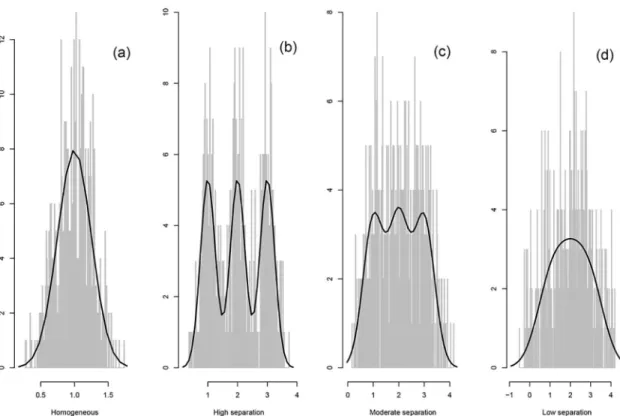
• Scenario A1: No clustering structure:K= 1 class withμ1= 1 andσ1= 0.25, seeFig 1(a).

• Scenario A2: High separation (s2

EðYjZÞ=s

2

Y ¼0:80, OVL = 0.06):K= 3 classes withμ1= 1,

μ2= 2,μ3= 3, andσ1=σ2=σ3= 0.25, seeFig 1(b).

• Scenario A3: Moderate separation (s2

EðYjZÞ=s

2

Y ¼0:70, OVL = 0.29):K= 3 classes with μ1= 1,μ2= 2,μ3= 3, andσ1=σ2=σ3= 0.4, seeFig 1(c).

• Scenario A4: Low separation (s2_EðYjZÞ=s2_Y ¼0:60, OVL = 0.74):K= 3 classes withμ1= 1,

μ2= 2,μ3= 3, andσ1=σ2=σ3= 0.7, seeFig 1(d).

In the base-case analysis, the data are simulated using equal class proportions (i.e.λj= 1/K

for each classj). The histograms of these simulated data for a randomly selected data set are displayed inFig 1, together with the true marginal densities. Separation decreases fromFig 1(b) to 1(d), to end in a unimodal distribution.

We implemented the criterion proposed by R&M, and we compared this criterion with the results of RJMCMC [12], DIC3and DIC4[11], and BIC. To establish whether a class is empty

under the R&M criterion we used different values for the cut-off (ψ) i.e., 0, 0.01, 0.02, and 0.05 of observations in the sample, and the maximum number of latent classes was set toKmax= 10.

The prior for the class proportionsλwas chosen to be a symmetric Dirichlet distribution with hyper-parameter equal toα= 0.00001, 0.001, 0.01, 0.05, 0.1, 0.3, 0.5, 0.9.

Fig 1. Univariate simulated data study. Histograms of randomly selected generated data sets. The solid lines represent

the true marginal densities. doi:10.1371/journal.pone.0168838.g001

For the priors of the class-specific means, we considered both a normal-gamma prior and a vague prior. The vague prior wasμj*N(0, 1000). The normal-gamma prior is a

hierarchi-cal data-dependent prior that places a normal prior on the prior mean and a shrinkage prior on the prior variance [16]. This prior for a univariate mixture model can be defined as fol-lows:

m_kjl;b0Nðb0;ZR 2_Þ;

whereη*Γ(ν1,ν2) andb0*N(m0,M0),m0andRare the median and range of the data,

respectively.M 1

0 is set to 0 (since this is not possible in practice here we setM 1

0 ¼10

7

). The hyper-parametersν1andν2are set to 0.5 to allow considerable shrinkage of the prior

variance of class means [16].

For the priors of the class-specific variance, we also considered a hierarchical data-depen-dent prior and a vague prior. The hierarchical data-dependata-depen-dent prior on the class-specific vari-ances was implemented by Malsiner-Walli et al. [16] in a multivariate mixture model, and is given by:

1=s2

kGðb1 ¼1:25;b2¼1=ð2C0ÞÞ;

whereC0*Γ(1= 0.25,2= 20/R2). The vague prior on the class-specific variances was

s2

j Uð0;10Þ.

We used a full factorial design to vary a) the number of latent classes and the degree of sepa-ration (using the four scenarios described above), b) the criterion for determining the number of latent classes (i.e. the R&M criterion with different cut-off values, RJMCMC, DIC3, DIC4,

and BIC), and c) the value ofαin the Dirichlet distribution (i.e.α= 0.00001, 0.001, 0.01, 0.05, 0.1, 0.3, 0.5, or 0.9).

Three additional factors were varied in sensitivity analyses. In these sensitivity analyses, only the scenario with high separation between classes was simulated, but the other factors in the full factorial design were not fixed.

Two sensitivity analyses consisted of a) changing the sample size of the data set (i.e. to 100 and 1000 observations) and b) simulating data with unequal proportions of the latent classes, including one small class, usingλ1= 0.475,λ2= 0.475,λ3= 0.05. Furthermore, we investigated

the sensitivity of the criteria to outlying values, by running Scenario A1 with two extreme val-ues added at each tail of the distribution. Finally, we also performed a sensitivity analysis for the number of latent classes, withKranging fromK= 1 toK= 6, withn= 100×Kand means chosen asμj=jforj= 1,. . .,Kandσj= 0.25 and alsoσj= 0.40.

We generated 50 data sets for each setting in the base-case analysis and the sensitivity analy-ses, except for the sensitivity analyses with varying number of clasanaly-ses, which used only 20 data sets. The low number of simulated data sets for these sensitivity analyses was necessary to limit the total computation time. MCMC sampling is run for each data set for 50,000 iterations after discarding the first 5,000 iterations (burn-in). Computations were performed using the follow-ing packages in R: rjags for the R&M criterion (seeS1andS2Figs in Supplementary Material Section), Rmixmod and lcmm for calculating BIC in a frequentist setting, and mixAK for the RJMCMC technique. To be able to compute DIC3and DIC4, an MCMC sampler for the

model parameters and the class assignments in the univariate mixture model was programmed in R. The programs of the simulation studies can be obtained by contacting the corresponding author.

Simulation study A: results

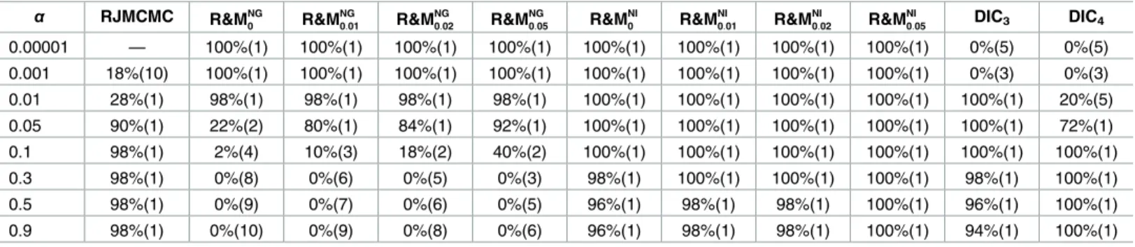
Table 1shows the simulation results of Scenario A1. This table presents the success rate (the percentage of data sets in which the true number of clusters was obtained) of the different approaches, the mode of the estimated number of classes is presented in parentheses. The cri-terion of Rousseau and Mengersen is denoted as R&MNGif hierarchical priors are used for both the class-specific mean and the class-specific variance, and as R&MNIif the vague priors are used for both the class-specific mean and the class-specific variance, with the cut-off value for defining a class to be empty as a subscript. For example,R&MNI

0:02represents the Rousseau

and Mengersen criterion with the vague priors for both the specific mean and the class-specific variance whereψ= 0.02.

In this scenario, the models cannot underestimate the number of classes. Small values forα for both a normal-gamma prior and a vague prior in the R&M criterion result in a better esti-mation of the true number of latent classes. However, the R&M criterion with a normal-gamma prior requires much lower values ofα(i.e.α<0.1) to obtain adequate results com-pared to the R&M criterion with the vague prior, in which any value ofαbelow 0.5 leads to good results. The other approaches (i.e. RJMCMC, DIC3, and DIC4) show better results with

larger values forα. In case of a very low value ofα, the convergence of the MCMC sampler in the RJMCMC method was poor and therefore no results are reported in the tables for this method withα= 0.00001.

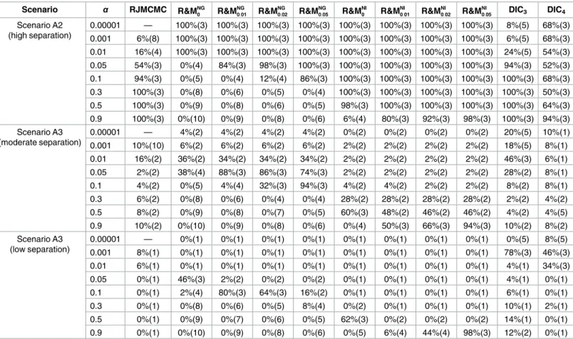
Table 2shows the simulation results of Scenario A2 (high separation), Scenario A3 (moder-ate separation), and Scenario A4 (low separation). In Scenario A2, small values forα(i.e.α<

0.05) in the R&M criterion result in a perfect estimation of the true number of latent classes. The number of classes is overestimated by the R&M criterion with the normal-gamma prior for higher values ofα. No such overestimation is observed for the vague prior. Similar results were obtained in the sensitivity analysis for the number of latent classes (seeS1andS2Tables). In that sensitivity analysis, the normal-gamma prior yielded good results with values ofα<

0.1, but the vague only gave good results for larger values ofα, withα>0.05. RJMCMC and DIC3gave the best results with larger values forα(α>0.1). The performance of DIC4does

not seem to depend on the value ofα, but it is not very good, with the probability of finding the true number of latent classes ranging from 50 to 70%. In the sensitivity analysis for the sample size, the number of classes is underestimated in case a low value ofαis used with a small sample size of 100 observations, but it is estimated accurately in the other situations (see

S3 Table).

Table 1. The results of Scenario A1. Percentage of data sets in which the true number of clusters was found, with the mode of the estimated number of

clas-ses in parentheclas-ses. α RJMCMC R&MNG0 R&M NG 0:01 R&M NG 0:02 R&M NG 0:05 R&M NI 0 R&M NI 0:01 R&M NI 0:02 R&M NI 0:05 DIC3 DIC4 0.00001 — 100%(1) 100%(1) 100%(1) 100%(1) 100%(1) 100%(1) 100%(1) 100%(1) 0%(5) 0%(5) 0.001 18%(10) 100%(1) 100%(1) 100%(1) 100%(1) 100%(1) 100%(1) 100%(1) 100%(1) 0%(3) 0%(3) 0.01 28%(1) 98%(1) 98%(1) 98%(1) 98%(1) 100%(1) 100%(1) 100%(1) 100%(1) 100%(1) 20%(5) 0.05 90%(1) 22%(2) 80%(1) 84%(1) 92%(1) 100%(1) 100%(1) 100%(1) 100%(1) 100%(1) 72%(1) 0.1 98%(1) 2%(4) 10%(3) 18%(2) 40%(2) 100%(1) 100%(1) 100%(1) 100%(1) 100%(1) 100%(1) 0.3 98%(1) 0%(8) 0%(6) 0%(5) 0%(3) 98%(1) 100%(1) 100%(1) 100%(1) 98%(1) 100%(1) 0.5 98%(1) 0%(9) 0%(7) 0%(6) 0%(5) 96%(1) 98%(1) 98%(1) 100%(1) 96%(1) 100%(1) 0.9 98%(1) 0%(10) 0%(9) 0%(8) 0%(6) 96%(1) 98%(1) 98%(1) 100%(1) 94%(1) 100%(1)

The success rate of BIC using a frequentist approach was 100%. doi:10.1371/journal.pone.0168838.t001

When looking at Scenario A3 (moderate separation) and Scenario A4 (low separation), a different picture emerges. These results show that the R&M criterion may underestimate the true number of latent classes for low values ofα. Namely, the R&M criterion with the normal-gamma prior underestimates the number of classes with low values ofαand overestimates this number with high values ofα. There is a narrow range around values ofα= 0.05 in which the performance of this criterion is good, and this range seems to depend on the cut-off for defin-ing a class to be empty. On the other hand, the R&M criterion with the vague prior almost always underestimates the number of latent classes in Scenario A3 and Scenario A4. Underes-timation rarely occurs with higher values ofα, but a large value forαmay result in overestimat-ing the true number of latent classes. In Scenario A4, in which the distribution of the data looks unimodal, all approaches exceptR&MNI

0:02andR&M NI

0:05perform poorly, and most

meth-ods detect only a single class.

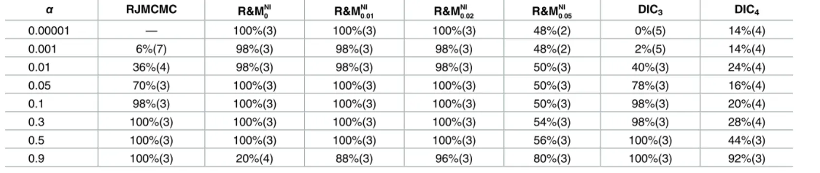
As a sensitivity analysis, we simulated a heterogeneous population with three unequal pro-portions, i.e.λ1= 0.475,λ2= 0.475,λ3= 0.05,μ1= 1,μ2= 2,μ3= 3 andσ1=σ2=σ3= 0.25 (high

separation), seeTable 3for the results. Here we performed the R&M criterion only with the vague prior. These results are consistent with the results of Scenario A2. The performance of the R&M criterion is quite good except forR&MNI

0:05since the smallest class proportion is 5%,

the cut-off defined for a class to be empty. Finally, in case a few outlying values were added to

Table 2. The results of Scenario A2–A4. Percentage of data sets in which the true number of clusters was found, with the mode of the estimated number of

classes in parentheses.

Scenario α RJMCMC R&MNG0 R&M NG 0:01 R&M NG 0:02 R&M NG 0:05 R&M NI 0 R&M NI 0:01 R&M NI 0:02 R&M NI 0:05 DIC3 DIC4 Scenario A2 (high separation) 0.00001 — 100%(3) 100%(3) 100%(3) 100%(3) 100%(3) 100%(3) 100%(3) 100%(3) 8%(5) 68%(3) 0.001 6%(8) 100%(3) 100%(3) 100%(3) 100%(3) 100%(3) 100%(3) 100%(3) 100%(3) 6%(5) 68%(3) 0.01 16%(4) 100%(3) 100%(3) 100%(3) 100%(3) 100%(3) 100%(3) 100%(3) 100%(3) 24%(5) 54%(3) 0.05 54%(3) 0%(4) 84%(3) 98%(3) 100%(3) 100%(3) 100%(3) 100%(3) 100%(3) 94%(3) 52%(3) 0.1 94%(3) 0%(5) 0%(4) 12%(4) 86%(3) 100%(3) 100%(3) 100%(3) 100%(3) 100%(3) 68%(3) 0.3 100%(3) 0%(8) 0%(6) 0%(5) 0%(4) 100%(3) 100%(3) 100%(3) 100%(3) 100%(3) 50%(3) 0.5 100%(3) 0%(9) 0%(8) 0%(6) 0%(5) 98%(3) 100%(3) 100%(3) 100%(3) 100%(3) 64%(3) 0.9 100%(3) 0%(10) 0%(9) 0%(8) 0%(6) 6%(4) 80%(3) 92%(3) 98%(3) 100%(3) 94%(3) Scenario A3 (moderate separation) 0.00001 — 4%(2) 4%(2) 4%(2) 4%(2) 0%(2) 0%(2) 0%(2) 0%(2) 20%(5) 10%(1) 0.001 10%(10) 6%(2) 6%(2) 6%(2) 6%(2) 2%(2) 2%(2) 2%(2) 2%(2) 18%(5) 8%(1) 0.01 16%(2) 36%(2) 34%(2) 34%(2) 34%(2) 2%(2) 2%(2) 2%(2) 2%(2) 46%(3) 6%(1) 0.05 2%(2) 38%(4) 88%(3) 86%(3) 74%(3) 2%(2) 2%(2) 2%(2) 2%(2) 28%(2) 8%(1) 0.1 4%(2) 0%(5) 4%(4) 32%(3) 94%(3) 4%(2) 4%(2) 2%(2) 2%(2) 8%(2) 8%(1) 0.3 6%(2) 0%(8) 0%(6) 0%(4) 0%(4) 28%(2) 28%(2) 28%(2) 28%(2) 2%(2) 4%(2) 0.5 8%(2) 0%(9) 0%(8) 0%(7) 0%(5) 60%(3) 48%(2) 46%(2) 46%(2) 4%(2) 4%(5) 0.9 10%(2) 0%(10) 0%(9) 0%(8) 0%(6) 0%(4) 50%(3) 66%(3) 94%(3) 10%(2) 8%(2) Scenario A3 (low separation) 0.00001 — 0%(1) 0%(1) 0%(1) 0%(1) 0%(1) 0%(1) 0%(1) 0%(1) 0%(5) 8%(5) 0.001 8%(1) 0%(1) 0%(1) 0%(1) 0%(1) 0%(1) 0%(1) 0%(1) 0%(1) 78%(3) 46%(3) 0.01 6%(1) 0%(1) 0%(1) 0%(1) 0%(1) 0%(1) 0%(1) 0%(1) 0%(1) 4%(1) 34%(3) 0.05 0%(1) 46%(3) 2%(2) 0%(2) 0%(2) 0%(1) 0%(1) 0%(1) 0%(1) 4%(1) 0%(1) 0.1 0%(1) 2%(4) 80%(3) 64%(3) 16%(2) 0%(1) 0%(1) 0%(1) 0%(1) 6%(1) 0%(1) 0.3 0%(1) 0%(8) 0%(6) 0%(5) 8%(4) 0%(2) 0%(1) 0%(1) 0%(1) 10%(1) 2%(1) 0.5 0%(1) 0%(9) 0%(7) 0%(6) 0%(5) 62%(3) 0%(2) 0%(2) 0%(2) 14%(1) 0%(1) 0.9 0%(1) 0%(10) 0%(9) 0%(8) 0%(6) 0%(5) 6%(4) 44%(4) 98%(3) 12%(2) 0%(1)

The success rates of BIC using a frequentist approach for high, moderate, and low levels of separation were 100%(3), 16%(2), and 0%(1), respectively. doi:10.1371/journal.pone.0168838.t002

the homogeneous data of Scenario A1, the outlying values were assigned to different classes when the cut-offψwas lower than 0.02 (seeS4 Table).

Simulation study B: a longitudinal study with a mixture of Gaussian

random effects distributions

Simulation study A enabled us to compare different criteria in a simple setting. However, mix-tures also appear in more complicated models, where it may be difficult to calculate some of the criteria that were evaluated in Simulation study A. However, the calculation of the R&M criterion should still be feasible in that case. To verify the performance of the R&M criterion we tested its performance based on a simulation study for a mixture model with longitudinal data.

In this simulation study we generate data from a growth mixture model, which is also known as a latent class mixed effects model [28,29] with a mixture model on the random effects [29]. The density function in a Gaussian growth mixture model can be expressed asEq 1, wherefj(y) is the density function that describes the trajectory for classj. The vectorθj

repre-sents the parameters that are associated with the trajectory of classj. The growth mixture model for individuals that belong to latent classjcan be expressed as:

yitjj ¼yj0þbij0þ ðyj1þbij1Þtimeitþit;

whereyit|jis thetth observation of theith individual, given that this individual is in latent class

j, respectively.θj0andθj1are the fixed intercept and slope of thejth latent class.bij0andbij1are

the random intercept and slope of thejth latent class that are assumed to be bivariate normally distributed with mean zero and a class-specific variance-covariance structure. The residualsit

are now assumed to be normally distributed, and independent of the random effects. Thus in this model the class-specific parameters (i.e.θjinEq 1) consist of the fixed intercept and slopes

and the variances and covariances of the random effects; the parameters common to all classes (i.e.γinEq 1) consist only of the variance ofit.

In this simulation study we computed the R&M criterion and the BIC. To establish whether a class is empty with the R&M criterion we used different values for the cut-off (ψ) as in Sec-tion ‘simulaSec-tion study A’ (i.e., 0, 0.01, 0.02, and 0.05 of observaSec-tions in the sample), and the maximum number of latent classes was also set toKmax= 10. Here we considered a

homoge-neous population (K= 1) and a heterogeneous population (K= 3).

Table 3. Unequal proportions heterogeneous scenario; a heterogeneous population with three clusters.λ1= 0.475,λ2= 0.475,λ3= 0.05,μ1= 1,μ2=

2,μ3= 3 andσ1=σ2=σ3= 0.25 (high separation). Percentage of data sets in which the true number of clusters was found, with the mode of the estimated

number of classes in parentheses.

α RJMCMC R&MNI 0 R&M NI 0:01 R&M NI 0:02 R&M NI 0:05 DIC3 DIC4 0.00001 — 100%(3) 100%(3) 100%(3) 48%(2) 0%(5) 14%(4) 0.001 6%(7) 98%(3) 98%(3) 98%(3) 48%(2) 2%(5) 14%(4) 0.01 36%(4) 98%(3) 98%(3) 98%(3) 50%(3) 40%(3) 24%(4) 0.05 70%(3) 100%(3) 100%(3) 100%(3) 50%(3) 78%(3) 16%(4) 0.1 98%(3) 100%(3) 100%(3) 100%(3) 50%(3) 98%(3) 20%(4) 0.3 100%(3) 100%(3) 100%(3) 100%(3) 54%(3) 98%(3) 28%(4) 0.5 100%(3) 100%(3) 100%(3) 100%(3) 56%(3) 100%(3) 44%(3) 0.9 100%(3) 20%(4) 88%(3) 96%(3) 80%(3) 100%(3) 92%(3)

The success rate of BIC using a frequentist approach was 98%(3). doi:10.1371/journal.pone.0168838.t003

• Scenario B1: (homogeneous data with a random intercept and slope):K= 1 class withθ10=

2 andθ11=−0.2, bi1*N2(0,S),S¼

0:252 0 0 0:0252

" #

and the residualsitare normally

distributed with variance of 0.252,it*N(0, 0.252), and independent of the random effects,

seeFig 2(a). The data were generated as

yitjj ¼yj0þbij0þ ðyj1þbij1Þtimeitþit;

and this model was also used for the analysis, with an unstructured random effects variance-covariance matrix. The class-specific parameters thus consisted of the fixed interceptθj0and

slopeθj1, as well as 3 parameters forS, so that d = 5.

• Scenario B2: (heterogeneous data with a random intercept):K= 3 classes withθ10= 1,θ20=

2,θ30= 3 andβ=−0.2,bij0*N(0, 0.252),bij1= 0 (a random intercept model) forj= 1, 2, 3

and the residualsitare normally distributed with variance of 0.252, i.e.,it*N(0, 0.252),

and independent of the random effects, seeFig 2(b). The data were generated as yitjj¼yj0þbij0þbtimeitþit;

and this model was also used for the analysis. The class-specific parameters thus consisted of the fixed intercept and the variance of the random intercept, so that d = 2.

• Scenario B3: (heterogeneous data with a random intercept and slope):K= 3 classes withθ10=

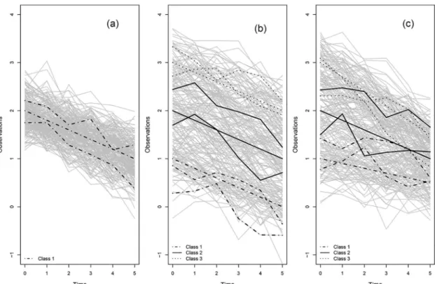
1,θ20= 2,θ30= 3 andθ11=−0.1,θ21=−0.2, andθ31=−0.3,bij0*N(0, 0.252), bij*N2(0,S), Fig 2. Longitudinal simulated data study. The left profile belongs to a homogeneous population with one class. The

middle one belongs to a population with three classes where classes differ only in intercept, and the right profile belongs to a heterogeneous population with three classes where classes differ both in intercept and slope.

S¼ 0:25

2 ₀

0 0:0252

" #

forj= 1, 2, 3 and the residualsitare normally distributed with

vari-ance of 0.252,it*N(0, 0.252), and independent of the random effects, seeFig 2(c). The data

were generated as

y_itjj¼yj0þbij0þ ðyj1þbij1Þtimeitþit;

and this model was also used for the analysis, with an unstructured random effects variance-covariance matrix. The class-specific parameters thus consisted of the fixed interceptθj0and

slopeθj1, as well as 3 parameters forS, so that d = 5.

Vague priors were specified for the class-specific parametersθj0andθj1, i.e.N(0, 103). An Γ−1

(10−3, 10−3) was specified for the variance of the residuals (this prior also used for the vari-ance of random intercept in Scenario B2). An Inv-Wishart(R, df) distribution was specified for the variance-covariance structure of the random intercept and random slope. We set the degrees of freedom, df, to 3 and the scale parameter matrix, R, to a diagonal matrix with small values, i.e. 10−3[30]. For the class membership probability a Dirichlet distribution with differ-ent values (i.e.,α= 0.00001, 0.001, 0.01, 0.05, 0.1, 0.3, 0.5, 1.0, 1.5, 2.0, and 2.5, whereKmax=

10) for the class proportions was specified. Larger values here were specified since in Scenario B1 and Scenario B3d= 5.

In this analysis, the data are simulated using equal class proportions (i.e.λj= 1/Kfor each

classj).Fig 2shows a randomly selected generated data set for the three scenarios.

In a sensitivity analysis, we also fitted the random intercept and slope model to the data of Scenario B2 (which were generated with only a random intercept). The purpose of this analysis was to investigate the performance of the criteria in case the statistical model does not match exactly with how the data were generated.

We generated 50 data sets for each setting consisting of 200 subjects and 6 observations per subject. MCMC sampling is run for each data set for 50,000 iterations after discarding the first 5,000 iterations (burn-in).

Simulation study B: results

The simulation results of Scenario B1 (homogeneous data with a random intercept and slope) show that the R&M criterion with the vague prior estimates the true number of classes per-fectly. The results of this simulation are presented inS5 Tablein Supplementary Material Section.

Table 4shows the simulation results of Scenario B2 (heterogeneous data with a random intercept). In this scenariod= 2, thereforeαshould be smaller than 1 to make sure that over-fitted classes become empty asymptotically [4]. In this scenario, large values forα(i.e. 0.1<α <0.9) in the R&MNIcriterion result in an accurate estimation of the true number of latent classes. An underestimation of the number of classes is observed for the R&MNIcriterion when a lower value ofαis used. In this scenario, different cut-offs lead to the same results.

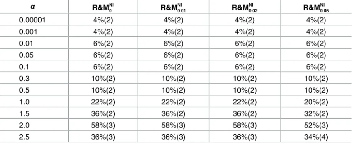
Table 5shows the simulation results of Scenario B3 (heterogeneous data with a random intercept and slope). In this scenariod= 5, thereforeαshould be smaller than 2.5. In this sce-nario, settingα= 2.0 in the R&MNIcriterion yields the most precise estimation of the true number of latent classes. Using this value forα, the result of the R&M criterion was better than BIC. An underestimation of the number of classes is observed for the R&MNIcriterion when a lower value ofαis used. Larger values forαlead to an overestimation of the true number of latent classes.

In the sensitivity analysis where a random intercept and slope model was fitted to data with only random intercept, choosingα= 2 led to good results (seeS6 Table), whereas in the analy-sis with a random intercept model, values ofαlower than 1 were necessary to prevent overesti-mation of the number of latent classes. These results support setting the value ofαslightly lower thand/2, wheredis the number of class-specific parameters of the model that is fitted to the data.

Simulation study A and B: conclusions

Simulation study A shows how the prior for the class-specific parameters and the Dirichlet prior for the class proportion interact to affect the selection of the correct number of latent class models. Using a hierarchical prior (i.e. a normal-gamma prior) for the class-specific means and variances, values for the Dirichlet hyperparameterαin the range 0.05–0.10 lead to acceptable results with both moderate or high separation between classes. Higher values forα may lead to an overestimation of the number of latent classes, even ifαremains well below the threshold valued/2 that was given in the proof of Rousseau and Mengersen [4]. Forα<0.05 a good performance is observed in the high separation scenario, but the number of classes is

Table 5. The results of Scenario B3. Percentage of data sets in which the true number of clusters was

found, with the mode of the estimated number of classes in parentheses.

α _R&MNI 0 R&M NI 0:01 R&M NI 0:02 R&M NI 0:05 0.00001 4%(2) 4%(2) 4%(2) 4%(2) 0.001 4%(2) 4%(2) 4%(2) 4%(2) 0.01 6%(2) 6%(2) 6%(2) 6%(2) 0.05 6%(2) 6%(2) 6%(2) 6%(2) 0.1 6%(2) 6%(2) 6%(2) 6%(2) 0.3 10%(2) 10%(2) 10%(2) 10%(2) 0.5 10%(2) 10%(2) 10%(2) 10%(2) 1.0 22%(2) 22%(2) 22%(2) 20%(2) 1.5 36%(2) 36%(2) 36%(2) 32%(2) 2.0 58%(3) 58%(3) 58%(3) 52%(3) 2.5 36%(3) 36%(3) 36%(3) 34%(4)

The success rate of BIC using a frequentist approach was 46%(3). doi:10.1371/journal.pone.0168838.t005

Table 4. The results of Scenario B2. Percentage of data sets in which the true number of clusters was

found, with the mode of the estimated number of classes in parentheses.

α R&MNI0 R&M NI 0:01 R&M NI 0:02 R&M NI 0:05 0.00001 4%(1) 4%(1) 4%(1) 4%(1) 0.001 4%(2) 4%(2) 4%(2) 4%(2) 0.01 18%(2) 18%(2) 18%(2) 18%(2) 0.05 48%(2) 48%(2) 48%(2) 48%(2) 0.1 74%(3) 74%(3) 74%(3) 74%(3) 0.3 90%(3) 90%(3) 90%(3) 90%(3) 0.5 96%(3) 98%(3) 98%(3) 100%(3) 0.9 8%(4) 14%(4) 20%(4) 34%(4)

The success rate of BIC using a frequentist approach was 98(3)%. doi:10.1371/journal.pone.0168838.t004

underestimated in scenarios with a moderate or low amount of separation. This underestima-tion of the number of latent classes with a low Dirichlet hyperparameter was not observed in a previous simulation study, however that study simulated only data sets with well separated latent classes [16].

With a vague prior for the class-specific means and variances, a perfect performance of the R&M criterion is observed in well separated data sets, irrespective of the value ofα. An under-estimation of the number of classes is observed in the scenarios with a low or moderate separa-tion, especially with low values forα. Settingαto a higher value, while still ensuring thatα<

d/2, led to a considerable improvement in the selection of the number of latent classes in these scenarios. In additional simulations (results not shown), we confirmed that settingαto a value above the threshold (i.e. toα>d/2) results in an overestimation of the number of latent clas-ses, as was predicted by the proof in Rousseau and Mengersen [4].

Using the normal-gamma prior, the performance of the R&M criterion seems quite sensi-tive to the value ofα. In addition, the optimal value ofα(i.e. that leads to highest probability of choosing the correct number of classes) depends on the separation between classes and the true number of classes, which are typically not known in practice (seeS7 Table). In contrast the performance of the R&M criterion with a vague prior seems much more stable, as long as the value ofαis close to but below the threshold ofd/2. Of the 4 possible values for the thresh-old to determine whether a class is empty (i.e.ψinEq 5), we found the best performance using a value of 0.01 in the scenario with a moderate separation (seeS8 Table). In the other scenarios there was no clear difference between the possible values ofψ. Therefore settingψ= between 0.02 and 0.05 seems reasonable, and a value in this range should allow for the detection of rela-tively small classes containing a few percent of the population.

Compared to alternative criteria for selecting the number of latent classes, the performance of the R&M criterion was good. The performance of BIC was generally inferior to that of the R&M criterion, especially in data sets with many latent classes and data sets with moderate or low separation. The performance of DIC3, DIC4and RJMCMC depends on the value ofα.

Although in some scenarios specific values ofαseem to lead to a good performance for these criteria, there is no value ofαthat leads a good performance across all scenarios.

Simulation study B confirms the conclusions of simulation study A. It shows that the R&M criterion can also be implemented in a more complex and realistic setting such as a growth mixture model for longitudinal data. The R&M criterion using vague priors for the class-spe-cific parameters andαsmaller than but close tod/2 (e.g. between 0.8 and 0.9d/2) yielded the best results, and outperformed BIC. However, the results were generally less good in Scenario B3, which has a more complex structure with random intercept and slope.

Hemoglobin longitudinal data

In this section, we apply the R&M criterion to a finite mixture model for hemoglobin (Hb) val-ues of blood donors. Our motivating application is the trajectory of Hb valval-ues of blood donors over successive donations. Blood donors experience a temporary reduction in their Hb value after donation. Therefore, a minimum 8 week interval between two donations is set by the blood bank, to allow the donor’s Hb value to recover to its pre-donation level. However, this interval seems to be too short since on average there is a declining trajectory in the Hb values for blood donors who donate regularly [31,32]. Therefore, a considerable proportion of pro-spective blood donors are temporarily deferred from donation each year due to low Hb values [33]. A Hb value of 8.4 mmol/l (135 g/l) and 7.8 mmol/l (125 g/l) for men and women, respec-tively, is widely accepted as the lower cut-off value of eligibility for donation to protect donors from anemia [34]. The previous studies showed that some individuals have a fast recovery,

which results in a relatively stable trajectory, whereas others have a slow recovery that yields a declining trajectory in their Hb values [35,36].

Here, we use a data set of longitudinally observed Hb values from 1 January 2005 to 31 December 2012 collected by Sanquin Blood Supply in the Netherlands. This data set is based on a self-administered questionnaire study aimed at gaining insight into characteristics and motivation of the Dutch donor population [37]. Here we randomly selected 200 new regis-tered male blood donors who have at least 5 visits to blood bank. These data are part of the Donor InSight study, for more details see [37]. The Donor InSight study was approved by the Medical Ethical Committee Arnhem-Nijmegen in the Netherlands, and all participants gave their written informed consent. These data are available in the Supporting Information files (seeS1 File).

A mixed-effects model with random intercept and slope may be able to capture the hetero-geneity between individuals in these data. However previous studies suggested that describing the total donor population using a single trajectory may oversimplify the complex growth pat-terns of this population [35,36]. Therefore, a growth mixture modeling approach, which accounts for different subgroups of donors, seems to be a more appropriate method for captur-ing differences in Hb trajectories between donors [35,36]. Here we implemented the R&M cri-terion with vague priors for the parameters. Different cut-offs (i.e. 0, 0.01, 0.02, and 0.05) were used to define a class to be empty.

Several factors are known to be associated with Hb and hence may be used as predictors, i.e., sex [38], season [39], age [38]. Here we model Hb trajectory based on number of donations in last two years (NODY2), the season donation took place (a binary value for cold = 1 and warm seasons = 0), time since previous donation (TSPD), and age of donor (years) at first visit. The class-specific parameters are the intercept and the effect of NODY2. The aim of the model is to assign each donor to one ofjgroups in such a way that donors with similar Hb tra-jectories are in the same group, and that the groups are most different from each other in terms of the Hb trajectory.

The growth mixture model for the trajectory of Hb levels of blood donors who belong to latent classjcan be expressed as:

Hbitjj¼yj0þbij0þg1Ageiþg2Seasonitþg3TSPDitþ ðyj1þbij1ÞNODY2itþit;

where Hbit|jis the predicted Hb level at thetth observation of theith individual, given that

this individual is in latent classj.θj0andθj1are the fixed intercept and slope (coefficients of

NODY2) of latent classj.bij0andbij1are the random intercept and slope of latent classjthat

are assumed to be bivariate normally distributed with mean zero and a class-specific variance-covariance structure. The residualsitare assumed to be normally distributed, and

indepen-dent of the random effects.

Prior specification

The priors for the model parameters were chosen as follows. Vague priors were specified for both the class-specific parametersθ’s and the non-class-specific parametersγ’s, i.e.N(0, 103). AnΓ−1₍₁₀−3_{, 10}−3_{) was specified for the variance of the residuals. An Inv-Wishart(R, df)}

distri-bution was specified for the variance-covariance structure of the random intercept and ran-dom slope. We set the degrees of freeran-dom, df, to 3 and the scale parameter matrix, R, to a diagonal matrix with small values, i.e. 10−3[30]. Since the number of class-specific parameters dis 5, for the class membership probability a Dirichlet distribution with different values for alpha (i.e., 1.0, 1.5, 2.0, and 2.5) was specified for the mixing proportions.

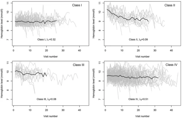
To analyze these data, we chose the results withα= 2, in view of the results of Scenario B3. Therefore, donors can be assigned to four different classes (seeTable 6). Based on the highest posterior probability, individuals were assigned to the latent classes after solving the label switching problem using the method suggested by Stephens [40]. This method was imple-mented in the “label.switching” package in R [41]. The profiles of these different classes are displayed inFig 3. This figure shows how trajectories of Hb values for blood donors are differ-ent. A group of donors have a low initial Hb value but relatively stable trajectory (Class I), donors in Class II have a very high initial Hb value and a very sharply declining trajectory. Donors in Class III have a high initial Hb value and a moderately declining trajectory, donors in Class IV have moderate initial Hb value and relatively stable trajectory. The results of this study regarding the number of latent classes and the interpretation of each class are supported by a previous study [35].

Fig 3. Hb profiles for four different classes.

doi:10.1371/journal.pone.0168838.g003

Table 6. Number of latent classes in Hb data for differentαand different cut-offs (ψ).

α _R&MNI 0 R&M NI 0:01 R&M NI 0:02 R&M NI 0:05 0.5 1 1 1 1 1.0 1 1 1 1 1.5 2 2 2 2 2.0 4 4 4 3 2.5 4 4 4 3

BIC using a frequentist approach found 2 classes. doi:10.1371/journal.pone.0168838.t006

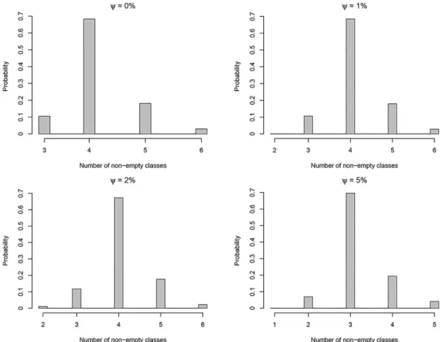
Fig 4shows the posterior distribution of the number of non-empty classes (K) for different cut-offs (ψ) using 50,000 MCMC iterations whenα= 2. This figure shows how the posterior mode of the number of nonempty classes may be affected by changing theψ.

Discussion

The results of the simulation studies showed that the R&M criterion has a high probability of estimating the correct number of latent classes, provided that the priors on the proportions and the class-specific parameters are chosen carefully. Despite the simplicity of this criterion, it performs at least as good as alternative selection criteria for the number of latent classes. The application of the R&M criterion to longitudinal data of blood donors further illustrated the practical usefulness of this method.

An important advantage of the R&M criterion is that this approach is straightforward to implement, using MCMC sampling for a mixture model with a large number of latent classes. The number of nonempty latent classes (i.e. classes with a proportion larger than the prede-fined cutoff value) is then an automatic byproduct of the MCMC sampler. Therefore, this cri-terion is easily implemented in standard Bayesian software such as WinBugs and JAGS, even for complex statistical models such as latent class mixed-effects models and multivariate mix-ture models. A further advantage of the R&M criterion is that it is not affected by label switch-ing. Despite the fact that the R&M criterion is relatively easy to implement, this criterion

Fig 4. Posterior distribution of non-empty classes (K) for different cut-offs (ψ).

seems to perform better than alternative criteria at estimating the true number of classes. Although only a limited set of statistical models was considered in the simulations, these results suggest that the R&M criterion works well and may be considered for practical use in Bayesian finite mixture models.

A strength of this study is that it is one of the first studies to compare different criteria for selecting the number of latent classes in a Bayesian setting. Although the R&M criterion has been implemented in simulated data previously [16], our study adds important insight into how this criterion should be implemented, based on a more elaborate simulation study with several scenarios. In a previous simulation study, it was shown that using a sufficiently low value ofα(e.g.α<0.001) prevents overfitting of the number of latent classes, and that using higher values ofα, withα<d/2 can lead to overfitting [16]. In that study, no underestimation of the number of latent classes was observed. In our simulation study we observed that with a slightly lower amount of separation between classes than in the previous study, underestima-tion of the number of classes often occurs, especially with low values ofα. This shows that the value ofαshould be chosen to provide a trade-off between the probability of overfitting and the probability of underfitting the number of latent classes. Unfortunately, no theoretical result is available on how the value of alpha affects the posterior distribution of the class sizes of clas-ses that are not overfitted. Furthermore we observed that if vague priors were used for the class-specific parameters, overfitting of the number of latent classes does not seem to occur, provided thatα<d/2.

Rousseau and Mengersen [4] proved that the class proportions converge to 0, not that they should be 0 with any data set of finite size. We therefore used different cut-offs for the propor-tions in a class to define a class to be empty. Using a cut-off of 0 may be sensitive to outlying values in the data and did not perform well in the simulation studies (seeS4 Table). In most applications, a cut-off of between 0.02 and 0.05 should be sufficient to make the criterion robust to outlying values, while being small enough to avoid the exclusion of real segments in the population. Although choosing the value of the cut-off in the range 0.02–0.05 is supported by results of the simulation studies, there are situations in which lower or higher values of the cut-off may be warranted. First, the interest of finding classes with small proportion may depend on the application and the research questions, and the value of the cut-off may be adapted accordingly. Second, in some applications there can be relevant prior information regarding the class sizes, e.g. if one suspects that there may be classes containing 1% of the pop-ulation, the cut-off should be set lower than 0.01. Finally, due to the asymptotic nature of the result of R&M, larger sample sizes would generally warrant lower values for the cut-off. How-ever, it should be noted that the rate of convergence proven by R&M is relatively slow, and val-ues of the cut-off between 0.02 and 0.05 seem to be realistic for a wide range of sample sizes. In case of sample sizes much larger than used in our simulation study, the possibility of lower val-ues of the cut-off may be considered. Therefore, in practice the value of the cut-off is to some extent a subjective decision to be made by the researcher, guided by prior knowledge and the level of interest in small subgroups.

Based on the results of the simulation studies, as discussed above, combined with the results of the blood donor data set, we give the following recommendations:

• We recommend to consider the R&M criterion to choose the number of latent classes in Bayesian finite mixture models. This criterion is easy to implement in practice, and its per-formance compares favorably with alternative criteria.

• To implement the criterion, one should first estimate a mixture model with a large number of classes (e.g. 10 classes), so that some classes will be overfitted.

• The number of classes in the final finite mixture model is then chosen as the posterior mode of the number of classes with a proportion larger than the predefined cut-off, which we rec-ommend to set between 0.02–0.05. Lower values of the cut-off should be used if the researcher is specifically interested in the classes with small proportions in the population. • It seems best to use vague priors for the class-specific parameters, and the use of hierarchical

priors such as the normal-gamma prior is not recommended.

• The class proportions should be given a Dirichlet prior withαlower than d/2, i.e. the num-ber of class-specific parameters divided by 2. A value ofαslightly lower than d/2 (e.g. between 0.8 and 0.9d/2) seems to yield the best results.

A limitation of this study is that only finite mixtures of Gaussian distributions and growth mixtures models were considered in the simulation study. Although the results of the simula-tion study were similar in these two types of models, it is not certain that the performance of the R&M will be similar in other types of models. Due to the large computation time associated with simulation studies in a Bayesian setting, it was not feasible to consider additional statisti-cal models. Another limitation is that only predefined settings were evaluated for the priors of both class-specific parameters and the class proportions. It is possible that intermediate values ofαorψ, or also other priors not considered here would lead to a better performance. We further did not consider alternatives to the normal-gamma prior and the vague prior for the class-specific parameters.

Conclusion

If appropriate priors are used for both the class-specific parameters and the class proportions, it seems possible to effectively estimate the number of latent classes in a Bayesian finite mixture model using the R&M criterion. This criterion compares favorably to alternative model selec-tion criteria for the number of latent classes in terms of both performance and ease of implementation.

Supporting Information

S1 Table. A heterogeneous population with different clusters (K= 1,. . ., 6).μj=jand

σj= 0.25, (j= 1,. . ., 6), and (Kmax= 10). Percentage of data sets in which the true number of

clusters was found, with the mode of the estimated number of classes in parentheses. A vague prior was used for the class-specific parameters.

(PDF)

S2 Table. A heterogeneous population with different clusters (K= 1,. . ., 6).μj=jand

σj= 0.25, (j= 1,. . ., 6), and (Kmax= 10). Percentage of data sets in which the true number of

clusters was found, with the mode of the estimated number of classes in parentheses. A nor-mal-gamma prior was used for the class-specific parameters.

(PDF)

S3 Table. The results of a sensitivity analysis for two different sample sizes i.e., n = 100 and n = 1000. Theses analyses are based on the Scenario A2. Percentage of data sets in which the

true number of clusters was found, with the mode of the estimated number of classes in paren-theses. A vague prior was used for the class-specific parameters.

(PDF)

S4 Table. The results of a sensitivity analysis for the outlying values. This analysis is based

in which the true number of clusters was found, with the mode of the estimated number of classes in parentheses. A vague prior was used for the class-specific parameters.

(PDF)

S5 Table. The results of Scenario B1. Percentage of data sets in which the true number of

clusters was found, with the mode of the estimated number of classes in parentheses. (PDF)

S6 Table. The results of a sensitivity analysis for fitting a more flexible model to the generated data. This analysis is based the Scenario B2 where the most flexible model (a

random intercept and slope model) is fitted to data to find the true number of classes. Per-centage of data sets in which the true number of clusters was found, with the mode of the estimated number of classes in parentheses. A vague prior was used for the class-specific parameters.

(PDF)

S7 Table. A heterogeneous population with different clusters (K= 1,. . ., 6).μj=jand

σj= 0.40, (j= 1,. . ., 6), and (Kmax= 10). Percentage of data sets in which the true number of

clusters was found, with the mode of the estimated number of classes in parentheses. A nor-mal-gamma prior was used for the class-specific parameters.

(PDF)

S8 Table. A heterogeneous population with different clusters (K= 1,. . ., 6).μj=jand

σj= 0.40, (j= 1,. . ., 6), and (Kmax= 10). Percentage of data sets in which the true number of

clusters was found, with the mode of the estimated number of classes in parentheses. A vague prior was used for the class-specific parameters.

(PDF)

S1 Fig. Bugs/Jags codes to implement a univariate Gaussian mixture model with R&M

cri-terion to find the true number of latent classes in Scenario A (R&MNI).

(TIF)

S2 Fig. Bugs/Jags codes to implement a latent class mixed-effects model with R&M

crite-rion to find the true number of latent classes in Scenario B (R&MNI).

(TIF)

S1 File. Hemoglobin longitudinal data.

(TXT)

Author Contributions