Domain Adaptation on the Statistical Manifold
Mahsa Baktashmotlagh
1,3, Mehrtash T. Harandi
2,3, Brian C. Lovell
1, and Mathieu Salzmann
3,2 1University of Queensland
2Australian National University
3NICTA
∗, Canberra
Abstract
In this paper, we tackle the problem of unsupervised domain adaptation for classification. In the unsupervised scenario where no labeled samples from the target domain are provided, a popular approach consists in transforming the data such that the source and target distributions be-come similar. To compare the two distributions, existing approaches make use of the Maximum Mean Discrepancy (MMD). However, this does not exploit the fact that prob-ability distributions lie on a Riemannian manifold. Here, we propose to make better use of the structure of this man-ifold and rely on the distance on the manman-ifold to compare the source and target distributions. In this framework, we introduce a sample selection method and a subspace-based method for unsupervised domain adaptation, and show that both these manifold-based techniques outperform the cor-responding approaches based on the MMD. Furthermore, we show that our subspace-based approach yields state-of-the-art results on a standard object recognition benchmark.
1. Introduction
In this paper, we propose to exploit the Riemannian structure of the space of probability distributions for unsu-pervised domain adaptation. Domain adaptation is crucial for the success of recognition methods in realistic scenarios. Indeed, in practice, the distribution of the test (target) sam-ples will often differ from the distribution of the training (source) samples. In visual recognition, this, for instance, is the case when the training and test images are acquired in very different conditions (e.g., studio versus home environ-ment, varying lighting conditions). As a consequence, in recent years, many solutions to this domain shift problem have been proposed [26, 27, 15, 14, 13].
In this work, we are interested in the problem of unsu-perviseddomain adaptation, where no labels are provided ∗NICTA is funded by the Australian Government as represented by the
Department of Broadband, Communications and the Digital Economy and the ARC through the ICT Centre of Excellence program.
for the target data. A natural approach to handling this sce-nario is to try and match the distributions of the source and target samples. To this end, two different approaches have been proposed: sample re-weighting and subspace extrac-tion. Sample re-weighting, or selection, methods [22, 13] assign weights to the source samples and optimize those weights so as to minimize a distance measure between the (re-weighted) source and target distributions. Subspace-based techniques [28, 2, 26] try to find a linear transfor-mation (or projection) of the source data, such that a dis-tance measure between the (transformed) source and target distributions is minimized. A popular choice of distance be-tween two distributions, and, to the best of our knowledge, the only one that has been used for domain adaptation, is the Maximum Mean Discrepancy (MMD) [16], which mea-sures the dissimilarity between two distributions as their maximum difference in expectation over a set of functions. The MMD is a simple yet powerful non-parametric criterion that compares the distributions of two sets of data by map-ping them to reproducing Kernel Hilbert Space (RKHS).
Although the MMD is endowed with nice properties, ac-cording to [16], the choice of kernel and kernel parame-ters is critical when using it as a test statistic. Non-optimal choices can lead to very poor estimates of the distance be-tween two distributions [16]. Furthermore, it does not truly consider the geometry of the space of probability distribu-tions. From information geometry, we know that proba-bility distributions lie on a Riemannian manifold known as the statistical manifold. Manifold-valued entities are often encountered in computer vision, e.g., covariance descrip-tors [33], linear subspaces [19], rotation matrices [20]. In all these different contexts, it has been consistently demon-strated that exploiting the Riemannian metric of the mani-fold to compare two entities was beneficial.
In this paper, we therefore propose to follow a similar intuition and to make use of the Riemannian metric on the statistical manifold as a measure of distance between the source and target distributions for domain adaptation.
A standard metric on the statistical manifold is the Fisher-Rao metric, which provides a mean to measure the
geodesic distance between two points on the manifold,i.e., two probability distributions. Utilizing the Fisher-Rao met-ric, however, is often impractical, since it requires having a parametric form of the distributions, which, in general, is unknown. To overcome this issue and simultaneously con-sider the geometry of the statistical manifold, we propose to make use of the Hellinger distance, which is closely re-lated to the Fisher-Rao metric in the sense that their intrinsic metrics are identical up to scale. Intuitively, its relation to the geodesic distance on the statistical manifold makes the Hellinger distance an attractive measure to compare proba-bility distributions.
In this setting, we introduce two formulations to domain adaptation: One based on sample re-weighting methods, and one inspired from subspace-based techniques. In both cases, we estimate the source and target distributions using kernel density estimation (KDE) and compare these distri-butions with the Hellinger distance. Our experimental eval-uation shows that our algorithms based on the Hellinger dis-tance outperform the corresponding ones that make use of the MMD. Furthermore, we show that our Hellinger dis-tance subspace method yields state-of-the-art results on the visual object recognition benchmark introduced in [30].
2. Related Work
Domain adaptation has received a lot of attention in re-cent years. The existing approaches can be roughly catego-rized into semi-supervised methods that rely on the avail-ability of a few labeled target samples, and unsupervised methods where only the source examples are labeled.
In the semi-supervised scenario, several studies have proposed to directly work on the final classifier and have thus modified existing algorithms, such as Support Vec-tor Machines (SVM) [12, 4] and other statistical classi-fiers [10, 9], to exploit the available labeled target exam-ples. Alternatively, metric learning [30], transformation learning [25] and dictionary learning [29] have been em-ployed. Several semi-supervised approaches have also been designed to handle the case where multiple source domains are available [11, 21]. Unfortunately, in many practical ap-plications, labeled target samples cannot be easily obtained. Unsupervised domain adaptation techniques therefore emerged as a solution to this challenging scenario where no labeled data is available from the target domain [34, 5, 8, 27]. In this setting, a popular and intuitive approach is to try and adapt the source samples so as to make the source and target distributions as similar as possible. The meth-ods that follow this line of research can be grouped into two categories. First, sample re-weighting [22], or selec-tion [13] approaches, which apply weights (binary in the case of sample selection) to the source samples to adjust their influence in the source distribution. Second, subspace-based methods [28, 2], which learn a linear transformation
of the features to modify the source and target distributions. Recently, a subspace-based approach was also introduced to tackle the case where the (labeled) source samples come from multiple distributions [26].
The above-mentioned sample re-weighting and subspace techniques make use of the MMD [16] as a distance mea-sure between two distributions, and therefore do not exploit the fact that probability distributions lie on a Riemannian manifold. This contradicts the evidence provided by many studies addressing different computer vision problems that accounting for the geometry of the manifold containing the data at hand helps improving the performance of many al-gorithms. This, for instance, is the case in object recogni-tion with covariance descriptors [33, 23], acrecogni-tion recognirecogni-tion on Grassmann manifolds [19], shape classification [31] and rotation averaging [20].
Riemannian geometry has, nonetheless, been exploited in domain adaptation. In particular, in [15], the source and target samples were summarized by subspaces, which are points on a Grassmann manifold. Intermediate subspaces were then generated by sampling points along the geodesic between the source and target subspaces. Classification was performed by using the projection of the original data on these subspaces. This approach was extended in [14] that showed that all the subspaces along the geodesic could be employed by forming the Geodesic Flow Kernel (GFK). Re-cently, the GFK was exploited in conjunction with a sample selection method [13]. All these manifold-based methods first map the data to a Grassmann manifold and then try to connect the points on the manifold. Distribution matching methods, however, seem more intuitive, since they directly model the domain shift phenomenon: Target samples and source samples are drawn from different distributions.
In this paper, we propose to follow the intuitive approach of distribution matching to better exploit the Riemannian structure of the statistical manifold. To this end, we intro-duce the use of the Hellinger distance in a sample selection and a subspace-based method. While the Hellinger distance has been employed for dimensionality reduction [7], to the best of our knowledge, our approach is the first attempt at exploiting the Riemannian geometry of the statistical mani-fold for domain adaptation.
3. Hellinger Distance on Statistical Manifolds
In this section, we review some concepts of Riemannian geometry on statistical manifolds. In particular, we focus on the derivation of the Hellinger distance, which will be used in our algorithms.Statistical manifolds are Riemannian manifolds whose elements are probability distributions. Loosely speaking, given a non-empty set X and a family of probability den-sity functions p(x|θ)parametrized by θ on X, the space
Fisher-Rao Riemannian metric onMis a function ofθand induces geodesics,i.e. curves with minimum length onM. In general, the parametrization of the PDFs of the data at hand is unknown, and choosing a specific distribution may not reflect the reality. This makes the Fisher-Rao metric ill-suited to measure the similarity between probability dis-tributions in practical scenarios1. Therefore, several stud-ies have opted for approximations of the Fisher-Rao met-ric. An important class of such approximations is the f -divergences, which can be expressed as
Df(pkq) = Z
f(p(x)
q(x))q(x)dx .
The (squared) Hellinger distance is a special case of f -divergences, obtained by taking f(t) = (√t−1)2. The (squared) Hellinger distance can thus be written as
D2H(pkq) = Z p p(x)−pq(x) 2 dx , (1)
which is symmetric, satisfies the triangle inequality and is bounded by 2 from above.
More importantly,
Theorem 1. The length of any curveγis the same under the Fisher-Rao metricDF Rand the Hellinger distanceDH up to a scale of 2.
Proof. Without any assumption on differentiability, let
(M, d) be a metric space. A curve in M is a continu-ous functionγ : [0,1] → M and joins the starting point
γ(0) =pto the end pointγ(1) =q. Our proof then relies on two theorems from [20] stated below.
Theorem 2([20]). If the intrinsic metrics induced by two metricsd1andd2are identical to scaleξ, then the length of any given curve is the same under both metrics up toξ.
Theorem 3([20]). Ifd1(p, q)andd2(p, q)are two metrics defined on a spaceM such that
lim
d1(p,q)→0
d2(p, q) d1(p, q)
= 1 (2)
uniformly (with respect topandq), then their intrinsic met-rics are identical.
According to [24], the asymptotic behavior of the Hellinger distance and the Fisher-Rao metric can be expressed as limp→qDH(p, q) = 0.5 ∗ DF R(p, q) +
O(DF R(p, q)3). This guarantees uniform convergence since the higher order terms are bounded and vanish rapidly independently of the path betweenpandq. It therefore di-rectly follows from Theorems 3 and 2 that the length of a curve underDH andDF R is the same up to a scale of 2, which concludes the proof.
1Note that, even with known parameters, computing the Fisher-Rao metric may not be feasible in closed-form.
3.1. Empirical Estimate of the Hellinger Distance
In a practical scenario, our goal is to compute the Hellinger distance between the distributionspandqwhen discrete observations are provided. In other words, we are interested in estimating Eq. 1 givennpsamples{xp i}drawn frompandnq samples{x
q
i}drawn fromq. In [6], it was shown that Eq. 1 can then be numerically approximated as
ˆ DH2 = 1 np np X i=1 q ˆ T(xpi)− q 1−Tˆ(xpi) 2 + 1 nq nq X i=1 q ˆ T(xqi)− q 1−Tˆ(xqi) 2 , (3)
whereTˆ(x) = ˆp(x)/ pˆ(x) + ˆq(x), withpˆ(x)andqˆ(x)the empirical estimates ofp(x)andq(x), respectively. Impor-tantly, this numerical approximation respects some of the properties of the true Hellinger distance [6]. In particular, it is symmetric and bounded by 2 from above.
In this work, we make use of kernel density estimation (KDE) with a Gaussian kernel to model the source and tar-get distributions. This lets us write
ˆ p(x) = 1 np np X j=1 1 p |2πHp|exp − (x−xpj)TH−p1(x−x p j) 2 ! , (4) whereHpis a diagonal matrix which can be computed,e.g., from the standard deviation of the data using the maximal smoothing principle [32]. A similar estimateqˆ(x)can be obtained from thenq samples{x
q
i}. We can then write
ˆ T(x) = 1 np Pnp j=1k(x, x p j) 1 np Pnp j=1k(x, x p j) + 1 nq Pnq j=1k(x, x q j) , (5)
wherek(·,·)is the Gaussian kernel function. This, in turn, lets us evaluate the squared Hellinger distance in Eq. 3.
4. Domain Adaptation on Statistical Manifolds
In this section, we introduce two approaches to unsu-pervised domain adaptation based on measuring distances between the source and target distributions on the statisti-cal manifold. The first method is inspired by sample selec-tion techniques, whereas the second one follows a subspace-based approach.In the remainder of this section, we denote by s(x)
and t(x) the probability density functions of the source samples Xs = xs1,· · · ,xsns
and target samplesXt =
xt
1,· · ·,xtnt
, respectively, where eachx∗i ∈RD.
4.1. Statistically Invariant Sample Selection (SISS)
As mentioned earlier, a popular approach to unsuper-vised domain adaptation consists in assigning weights to the
source samples in order to minimize the distance between the re-weighted source distribution and the target distribu-tion [22]. More recently, it was shown that selecting land-marks among the source samples, which is equivalent to us-ing binary weights, was even more effective [13]. Note that, in [13], sample selection was then followed by exploiting multiple GFKs. Here, we follow a similar sample selection idea, but make use of the Hellinger distance instead of the MMD. Furthermore, to provide a more direct comparison with MMD-based approaches, we do not make use of GFKs in a second stage. As will be shown in our experiments, the use of the Hellinger distance itself makes this GFK stage unnecessary.
More specifically, let α = [α1, . . . , αn], with αi ∈ {0,1}, be the vector of indicator variables for the data points in the source domain. In other words, if αi = 1, thenxs
i is considered to be a landmark. We seek to select the landmarks whose distribution is as similar as possible to the target distribution. To this end, we exploit the Hellinger distance on the statistical manifold. This lets us write the optimization problem min α 1 Pns i=1αi ns X i=1 αi q ˆ T(xs i)− q 1−Tˆ(xs i) 2 + 1 nt nt X i=1 q ˆ T(xt i)− q 1−Tˆ(xt i) 2 s.t. αi ∈ {0,1}, ∀1≤i≤ns (6) 1 Pns i=1αi ns X i=1 αiyi,c= 1 ns ns X i=1 yi,c, ∀1≤c≤C ,
whereyi,c is a binary variable indicating whether theith source sample belongs to classcor not, andCis the total number of classes. The second set of constraints enforces the proportions of source samples per class to remain the same as in the original data [13].
To fully cancel the influence of unselected source sam-ples, the weights should also be introduced in the KDE of both distributions. This implies modifying the definition of
ˆ
T(x)in Eq. 5, which then becomes
ˆ T(x) = 1 Pns j=1αj Pns j=1αjk(x, x s j) 1 Pns j=1αj Pns j=1αjk(x, xsj) + 1 nt Pnt j=1k(x, x t j) .
Note that, for notational convenience, we omit the explicit dependency ofTˆ(x)onα when writing our optimization problems. This dependency is, however, accounted for when we solve the optimization problem.
Solving the optimization problem (6) with binary
con-straints is intractable. Instead, we solve the relaxed problem
min β ns X i=1 βi q ˆ T(xs i)− q 1−Tˆ(xs i) 2 + 1 nt nt X i=1 q ˆ T(xt i)− q 1−Tˆ(xt i) 2 s.t. βi∈[0,1], ∀1≤i≤ns ns X i=1 βi = 1 (7) ns X i=1 βiyi,c= 1 ns ns X i=1 yi,c, ∀1≤c≤C .
whereβi is a variable that replacesαi/(Pαi)in the pre-vious formulation. In practice, we make use of Matlab’s solverfminconto solve the nonlinear problem (7) and ob-tain the binary weightsαby thresholdingβ.
Given the binary weights, we then simply train an SVM classifier on the selected source samples and obtain the la-bels for the target samples with this classifier.
4.2. Statistically Invariant Embedding (SIE)
Instead of re-weighting, or selecting, source samples, learning a linear transformation of the input features has also proven effective for domain adaptation [28, 2, 26]. Here, we follow this idea, but, again, exploit the distance on the statistical manifold instead of making use of the MMD as was done in previous approaches. Ultimately, our goal is to find a representation of the data that is invariant across the source and target domains, and would therefore be well-suited for classification. To this end, we seek to project the data to a low-dimensional latent space shared by both do-mains, such that the distance between the source and target distributions in this latent space is minimal.More specifically, we model the mapping of the data to a
d-dimensional space with a projection matrixW ∈RD×d,
withd < D. We then search for the projection that mini-mizes the Hellinger distance between the source and target distributions in the latent space. This can be expressed as
min W 1 ns ns X i=1 q ˆ T(WTxsi)− q 1−Tˆ(WTxsi) 2 + 1 nt nt X i=1 q ˆ T(WTxt i)− q 1−Tˆ(WTxt i) 2 s.t. WTW =I. (8)
Note that, here, we constrainW to be orthonormal, which typically avoids degeneracies, such as having all samples collapsing to the origin. Such constraints have proven ef-fective in many dimensionality reduction methods, such as Principal Component Analysis (PCA), as well as in
subspace-based domain adaptation methods [28, 2, 26]. Note also that, since we compute the matricesHsandHt in the KDE of the source and target distributions (see Eq. 4) using the standard deviations of the data, these matrices be-come functions of W to measure these deviations in the latent space.
The optimization problem (8) is formulated using purely unsupervised data, in the sense that even the source labels are not exploited. However, since our goal is classification, it would seem natural to encode the class information in the resulting latent space. This can be achieved by encouraging clustering in the latent space of the source samples belong-ing to the same class, which can be expressed in terms of the distance between the source samples in each class and the class mean. This yields the optimization problem
min W ˆ DH2(WTXs,WTXt) +λ C X c=1 nc X i=1 W T(xs i,c−µc) 2 s.t. WTW =I, (9)
whereCis the number of classes,nc the number of exam-ples in classc,xsi,cdenotes theithexample of classc, and µcthe mean of the examples in classc.
Problems (8) and (9) are nonlinear, constrained opti-mization problems. To account for the constraints, we re-formulate them as unconstrained nonlinear problems on the Grassmann manifold G(d, D). The Grassmann manifold
G(d, D)is the space of alld-dimensional subspaces ofRD. In contrast to Stiefel manifolds, on a Grassmann manifold, two subspaces that are identical up to a rotation correspond to the same point. This perfectly fits our needs, since global rotation of the data is irrelevant for our purpose.
To effectively solve such nonlinear optimization prob-lems, we make use of a conjugate gradient (CG) method on the manifold, which has been shown to typically have better convergence behavior than iterative projection methods [1]. Without going into the details, which can be found in [1], the main steps of such an algorithm can be described as:(i)
compute the gradient of the objective function on the mani-fold,(ii)determine a search direction based on this gradient, and(iii)perform a line search along a geodesic on the mani-fold. Note that the gradient on the manifold is obtained from the usual gradient of the objective function with respect to W. CG on the Grassmann manifold typically converges in 10-15 iterations in our experiments.
GivenW, we train an SVM classifier on the source sam-ples projected to the latent space and use this classifier on the projected target samples to estimate their labels.
5. Experiments
We evaluated our two approaches on the tasks of vi-sual object recognition and WiFi localization, and com-pared their performance against the state-of-the art methods
in each task. In the following, we refer to our sample selec-tion approach as SISS, and to our subspace-based approach as SIE, or SIE-CC when the class-clustering term was uti-lized,i.e., whenλ >0in (9).
In all our experiments, we used the Maximum Smooth-ing Principle to determine the bandwidths of the kernels in KDE. For the final classification, we used an SVM classi-fier with an RBF kernel whose variance σwas set to the median squared distance between the source examples, af-ter projection in the case SIE. For SIE, we used the sub-space disagreement measure of [14] to determine the di-mensionality of the projection matrixW. When using the class-clustering regularizer, the weightλwas set to1/(Cσ), whereCis the number of classes. In all our experiments, we first applied PCA jointly on the source and target sam-ples, kept all the variance of the data, and used the resulting representation as features.
5.1. Visual Object Recognition
To evaluate our methods on the task of visual object recognition, we used the benchmark domain adaptation dataset introduced in [30]. This dataset consists of four different domains: Caltech, Amazon, DSLR and Webcam. The Caltech [18] domain consists of 256 object classes with images downloaded from Google. The Amazon domain contains 31 classes, each of which includes different ob-ject instances seen from one canonical viewpoint. These images were obtained in a closely monitored environment with studio lighting conditions and have large intra-class variations. The DSLR domain also has 31 categories and contains images acquired with a digital SLR camera in a re-alistic environment under natural light. The images in the Webcam domain were captured in a similar environment as the DSLR ones. However, they have much lower resolution and contain significant noise. To perform object recogni-tion, the 10 object classes common to all four datasets were selected [14], which yields 2533 images in total. For each domain, each class contains between 8 and 151 images.
In our experiments, we used the image features provided by [14], which were extracted as described in [30]. In short, all images were resized and converted to grayscale, and the SURF detector [3] was employed to detect local scale-invariant interest points. A codebook of size 800 was then constructed from a subset of the Amazon dataset us-ing k-means clusterus-ing on 64-dimensional rotation invariant SURF descriptors extracted from the image patch around each interest point. The final feature vector for each im-age was taken as the normalized histogram of visual words obtained from this codebook.
We first evaluated our sample selection approach using the evaluation protocol introduced in [13]. This protocol was inspired by the fact that selecting landmarks requires a sufficient number of source examples [13]. Therefore, in
Method A→C A→D A→W C→A C→D C→W W→A W→C W→D NO ADAPT-1NN 26 25.5 29.8 23.7 25.5 25.8 23 20 59.2 NO ADAPT-SVM 41.7 41.4 34.2 51.8 54.1 46.8 31.1 31.5 70.7 LM[13] 45.5 47.1 46.1 56.7 57.3 49.5 40.2 35.4 75.2 KMM[17] 42.2 42.7 42.4 48.3 53.5 45.8 31.9 29.0 72.0 KMM-LM 44.0 47.1 45.0 54.1 52.2 49.1 40.4 32.8 78.9 SISS 44.4 49.0 46.8 55.1 54.8 54.9 39.9 33.7 87.3
Table 1. Recognition accuracies of landmark selection approaches on 9 pairs of source/target domains using the evaluation protocol of [13].C: Caltech,A: Amazon,W: Webcam,D: DSLR.
Method A→C A→D A→W C→A C→D C→W W→A W→C W→D NO ADAPT-1NN 26 25.5 29.8 23.7 25.5 25.8 23 20 59.2 NO ADAPT-SVM 41.7 41.4 34.2 51.8 54.1 46.8 31.1 31.5 70.7 GFK-SVM[14] 42.2 42.7 40.7 44.5 43.3 44.7 31.8 30.8 75.6 TCA[28] 35.0 36.3 27.8 41.4 45.2 32.5 24.2 22.5 80.2 DIP[2] 47.4 50.3 47.5 55.7 60.5 58.3 42.6 34.2 88.5 DIP-CC[2] 47.2 49.04 47.8 58.7 61.2 58 40.9 37.2 91.7 SIE 48.2 49.1 48.1 56.7 61.2 58 42.7 38.6 93 SIE-CC 47.6 49.04 47.8 57.6 61.2 57.3 42.4 36.2 93
Table 2. Recognition accuracies of subspace learning approaches on 9 pairs of source/target domains using the evaluation protocol of [13].
C: Caltech,A: Amazon,W: Webcam,D: DSLR.
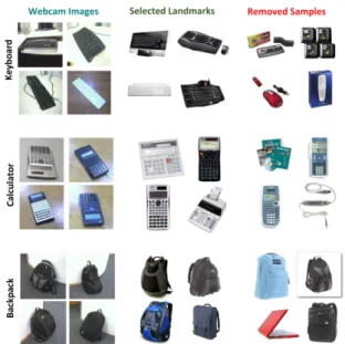
the source domain, all the samples in all the classes are employed. Furthermore, since the DSLR dataset contains fewer images, it is never used as a source domain. We compared the results of our SISS approach with those ob-tained by the landmark method of [13] (LM) and with ker-nel mean matching (KMM) [17], a sample re-weighting ap-proach that exploits MMD to compare the source and tar-get distributions. Furthermore, we also modified KMM to solve the same optimization problem as us, but with the MMD distance instead of the Hellinger one. We refer to this method as KMM-LM, since it also relies on binary weights. In Table 1, we show the recognition accuracies for the 9 pairs of source and target domains. Note that our SISS ap-proach outperforms KMM-LM in almost all cases. This ev-idences the benefits of exploiting the geometry of the sta-tistical manifold when comparing the source and target dis-tributions. Note also that KMM-LM performs better than the original KMM approach. Finally, our SISS approach achieves similar results as the more involved LM method, which relies on computing multiple GFKs based on the se-lected landmarks. Since the initial step of LM corresponds to KMM-LM, we conjecture that our results could be fur-ther improved by also making use of GFKs. This, however, goes beyond the scope of this paper. Fig. 1 shows the sam-ples that SISS selected or removed when using Amazon as source domain and Webcam as target one.
We then evaluated our subspace learning approach using the same protocol as before. In Table 2, we compare the results of our SIE approach with those obtained by other subspace-based methods. Our direct competitor in this case is DIP [2], which solves a similar optimization problem as
us, but exploits the MMD. Note that we achieve comparable or higher accuracy as DIP on the 9 different source/target pairs. Finally, we also evaluated our approach using the more standard protocol introduced in [30], where a subset of the source samples in each class is randomly selected. In Tables 3 and 4, we report the average accuracy over 20 different random splits for all the source/target pairs. Note that, here, our SIE approach more consistently outperforms the baselines. In particular, we outperform DIP, which, to the best of our knowledge, represents the state-of-the-art on the dataset. This evidences the importance of using an accu-rate metric on the statistical manifold when fewer samples are available.
5.2. Cross-domain WiFi Localization
To evaluate our approach on a different domain adapta-tion task, we used the WiFi dataset published in the 2007 IEEE ICDM Contest for domain adaptation [35]. The goal here is to estimate the location of mobile devices based on the received signal strength (RSS) values from different ac-cess points. The different domains represent two different time periods during which the collected RSS values may have different distributions. The dataset contains 621 la-beled examples collected during time period A (i.e., the source) and3128unlabeled examples collected during time period B (i.e., the target). We followed the transductive set-ting of [28], which uses all the samples from the source and
400random samples from the target.
In this case, we report the mean Average Error Distance (AED) over 10 random selections of target samples. The AED is computed as AED =
P
il(xi)−yi
Method A→C A→D A→W C→A C→D C →W NO ADAPT-1NN 22.6±0.3 22.2±0.4 23.5±0.6 20.8±0.4 22±0.6 19.4±0.7 NO ADAPT-SVM 38.7±1.6 36.7±2.3 37.2±2.8 44.3±2.4 41.1±3.9 39.9±3.2 GFS[15] 35.6±0.4 34.9±0.9 34.4±0.9 36.9±0.5 35.2±1 33.9±1.2 GFK-1NN[14] 37.9±0.4 35.2±0.9 35.7±0.9 40.4±0.7 41.1±1.3 35.8±1 GFK-SVM[14] 39±1.7 34.1±2.6 40.7±3.7 47.2±2.3 38.5±2.7 38.8±3.2
DLDA[27] 40.4±0.5 N/A 37.9±0.9 45.4±0.3 42.3±0.4 N/A
TCA[28] 40±1.3 39.1±1.5 40.1±1.2 46.7±1.1 41.4±1.2 36.2±1.0
DIP[2] 43.3±1.4 42.8±2.5 46.7±2.7 50±3.2 49±2.9 47.6±3.5
DIP-CC[2] 43.2±2.8 43.3±3.3 47.8±4.8 51.8±2.6 51.4±4.1 47.7±4.4
SIE 44.5±1.7 43.2±0.9 48.6±2.3 51.9±1.4 52.5±2.9 47.3±4.6
SIE-CC 44.4±1.4 43.1±1.9 48.5±2.6 52.3±1.1 53±2.3 48.1±4.3
Table 3. Recognition accuracies subspace learning approaches on 6 pairs of source/target domains using the evaluation protocol of [30].
C: Caltech,A: Amazon,W: Webcam,D: DSLR.
Method D→A D→C D→W W →A W →C W →D NO ADAPT-1NN 27.7±0.4 24.8±0.4 53.1±0.6 20.7±0.6 16.1±0.4 37.3±1.2 NO ADAPT-SVM 33.6±1.7 31.1±0.9 75.2±2.6 36.9±1.2 33.4±1.1 80.2±2.5 GFS[15] 32.6±0.5 30±0.2 74.9±0.6 31.3±0.7 27.3±0.5 70.7±0.9 GFK-1NN [14] 36.2±0.4 32.7±0.4 79.1±0.7 35.5±0.7 29.3±0.4 71.2±0.9 GFK-SVM [14] 39±1.1 34.5±0.8 76.2±1.2 40.8±1.2 36.1±0.9 72.4±2.2
DLDA[27] 39.1±0.5 N/A 86.2±1.0 38.3±0.3 36.3±0.3 N/A
TCA[28] 39.6±1.2 34±1.1 80.4±2.6 40.2±1.1 33.7±1.1 77.5±2.5
DIP[2] 40.5±1 39±0.5 86.7±1.2 42.5±1.5 37±0.9 86.4±1.8
DIP-CC[2] 41±0.9 35.8±0.6 84.02±0.9 41.1±1.1 37.1±0.9 85.3±2.5
SIE 39.1±0.6 38.9±0.4 88.6±1.0 44.1±0.8 39.9±0.7 89.3±0.5
SIE-CC 39.4±1.1 38.8±0.3 88.8±1.0 44.3±0.9 39.3±0.5 89.1±0.6
Table 4. Recognition accuracies subspace learning approaches on the remaining 6 pairs of source/target domains using the evaluation protocol of [30].C: Caltech,A: Amazon,W: Webcam,D: DSLR.
Figure 1. Samples selected as landmarks or removed by SSIS with Amazon as source domain and Webcam as target one.
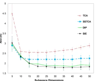
vector of RSS values,l(xi)is the predicted location andyi the corresponding ground truth location. Note that, here, all results were obtained with a nearest-neighbor classifier to follow the procedure of [28]. Fig. 2 depicts the accuracy as a function of the dimensionality of the learned subspace for several subspace-based methods. As before, we outper-form the MMD-based baselines (i.e., TCA and DIP). Impor-tantly, we also outperform the results obtained by the semi-supervised approach SSTCA. The mean AED of the sample selection approaches (which do not depend on any subspace dimension) are5.2±0.7for KMM-LM and4.8±0.4for our SISS approach. This again shows the benefits of using the metric on the statistical manifold.
6. Conclusion and Future Work
In this paper, we have proposed to exploit the structure of the space of probability distributions for unsupervised domain adaptation. In particular, we have considered the case of the Hellinger distance, which accurately approx-imates the Riemannian metric on the statistical manifold. We have then introduced a sample selection method and a subspace-based technique that exploit this measure to
com-Figure 2. Comparison of subspace learning approach (SIE) on the task of WiFi localization.
pare the distributions of the source and target samples. Our experimental evaluations have evidenced that the use of a geometry-aware metric yields improved recognition accu-racies. In the future, we intend to study how such a metric can be combined with more sophisticated domain adapta-tion methods based on the GFK, or on dicadapta-tionary learning.
References
[1] P. Absil, R. Mahony, and R. Sepulchre. Optimization Al-gorithms on Matrix Manifolds. Princeton University Press, 2008.
[2] M. Baktashmotlagh, M. Harandi, B. Lovell, and M. Salz-mann. Unsupervised domain adaptation by domain invariant projection. InICCV, 2013.
[3] H. Bay, T. Tuytelaars, and L. Van Gool. Surf: Speeded up robust features. InECCV, 2006.
[4] A. Bergamo and L. Torresani. Exploiting weakly-labeled web images to improve object classification: a domain adap-tation approach. InNIPS, 2010.
[5] L. Bruzzone and M. Marconcini. Domain adaptation prob-lems: A dasvm classification technique and a circular valida-tion strategy.TPAMI, 2010.
[6] K. Carter.Dimensionality reduction on statistical manifolds. 2009.
[7] K. Carter, R. Raich, W. Finn, and A. Hero. Fine: Fisher information nonparametric embedding.PAMI, 2009. [8] M. Chen, K. Weinberger, and J. Blitzer. Co-training for
do-main adaptation. InNIPS, 2011.
[9] H. Daum´e III, A. Kumar, and A. Saha. Co-regularization based semi-supervised domain adaptation. InNIPS, 2010. [10] H. Daum´e III and D. Marcu. Domain adaptation for
statisti-cal classifiers.JAIR, 2006.
[11] L. Duan, I. Tsang, D. Xu, and T. Chua. Domain adapta-tion from multiple sources via auxiliary classifiers. InICML, 2009.
[12] L. Duan, I. Tsang, D. Xu, and S. Maybank. Domain transfer svm for video concept detection. InCVPR, 2009.
[13] B. Gong, K. Grauman, and F. Sha. Connecting the dots with landmarks: Discriminatively learning domain-invariant fea-tures for unsupervised domain adaptation. InICML, 2013. [14] B. Gong, Y. Shi, F. Sha, and K. Grauman. Geodesic flow
kernel for unsupervised domain adaptation. InCVPR, 2012. [15] R. Gopalan, R. Li, and R. Chellappa. Domain adaptation for object recognition: An unsupervised approach. InICCV, 2011.
[16] A. Gretton, K. Borgwardt, M. Rasch, B. Sch¨olkopf, and A. Smola. A kernel two-sample test.JMLR, 2012.
[17] A. Gretton, A. Smola, J. Huang, M. Schmittfull, K. Borg-wardt, and B. Sch¨olkopf. Covariate shift by kernel mean matching.J. Royal. Statistical Society, 2009.
[18] G. Griffin, A. Holub, and P. Perona. Caltech-256 object cat-egory dataset. Technical report, Calif. Inst. of Tech., 2007. [19] M. Harandi, C. Sanderson, S. Shirazi, and B. Lovell.
Ker-nel analysis on grassmann manifolds for action recognition.
PRL, 2013.
[20] R. Hartley, J. Trumpf, Y. Dai, and H. Li. Rotation averaging.
IJCV, 2013.
[21] J. Hoffman, B. Kulis, T. Darrell, and K. Saenko. Discovering latent domains for multisource domain adaptation. InECCV, 2012.
[22] J. Huang, A. J. Smola, A. Gretton, K. Borgwardt, and B. Scholkopf. Correcting sample selection bias by unlabeled data. InNIPS, 2007.
[23] S. Jayasumana, R. Hartley, M. Salzmann, H. Li, and M. Ha-randi. Kernel methods on the riemannian manifold of sym-metric positive definite matrices. InCVPR, 2013.
[24] R. Kass. The geometry of asymptotic inference. Statistical Science, 1989.
[25] B. Kulis, K. Saenko, and T. Darrell. What you saw is not what you get: Domain adaptation using asymmetric kernel transforms. InCVPR, 2011.
[26] K. Muandet, D. Balduzzi, and B. Sch¨olkopf. Domain gener-alization via invariant feature representation. InICML, 2013. [27] J. Ni, Q. Qiu, and R. Chellappa. Subspace interpolation via dictionary learning for unsupervised domain adaptation. In
CVPR, 2013.
[28] S. Pan, I. Tsang, J. Kwok, and Q. Yang. Domain adaptation via transfer component analysis.TNN, 2011.
[29] Q. Qiu, V. Patel, P. Turaga, and R. Chellappa. Domain adap-tive dictionary learning. InECCV. 2012.
[30] K. Saenko, B. Kulis, M. Fritz, and T. Darrell. Adapting vi-sual category models to new domains. InECCV, 2010. [31] A. Srivastava, I. Jermyn, and S. Joshi. Riemannian analysis
of probability density functions with applications in vision. InCVPR, 2007.
[32] G. Terrell. The maximal smoothing principle in density esti-mation.J. of the American Statistical Association, 1990. [33] O. Tuzel, F. Porikli, and P. Meer. Pedestrian detection via
classification on riemannian manifolds.PAMI.
[34] D. Xing, W. Dai, G. Xue, and Y. Yu. Bridged refinement for transfer learning. InECML, 2007.
[35] Q. Yang, J. Pan, and V. Zheng. Estimating location using wi-fi.IEEE Intelligent Systems, 2008.
![Table 2. Recognition accuracies of subspace learning approaches on 9 pairs of source/target domains using the evaluation protocol of [13].](https://thumb-us.123doks.com/thumbv2/123dok_us/9440582.2818280/6.918.116.778.284.442/recognition-accuracies-subspace-learning-approaches-domains-evaluation-protocol.webp)