Bayesian Nonlinear Regression Models based on Slash Skew-t Distribution

European Online Journal of Natural and Social Sciences 2015; www.european-science.com Vol.4, No.1 Special Issue on New Dimensions in Economics, Accounting and Management

ISSN 1805-3602

Openly accessible at http://www.european-science.com 230

Bayesian Nonlinear Regression Models based on Slash Skew-t Distribution

Siavash Pirzadeh Nahooji 1_{, Rahman Farnoosh}2*_{, Nader Nematollahi}3

1_{Department of Statistics, Science and Research Branch, Islamic Azad University, Tehran, Iran;} 2_{School of Mathematics, Iran University of Science and Technology, Narmak, Tehran, Iran;}

3_{Department of Statistics, Allameh Tabataba'i University, Tehran, Iran.} *E-mail: [email protected].

Abstract

This paper considers the Bayesian analysis for estimating the parameters of nonlinear regression model when the error term has a slash skew-t distribution. This model is an asymmetric nonlinear regression model which is suitable for fitting the data sets with heavy tail and skewness. The properties of this model are derived and a hierarchical representation of this model based on the stochastic representation of slash skew-t distribution is given. This representation allows us to use Markov Chain Monte Carlo method to estimate the parameters of model. To compare this model with other asymmetric nonlinear regression models, we use conditional predictive ordinate statistic and deviance information, expected Akaike information and expected Bayesian information criterions, and show the performance of the proposed model by a simulation study. Also an application of the new model to fitting a real data set is discussed.

Keywords: Bayesian analysis, Nonlinear regression models, Slash skew-t distribution, Skew slash distribution, Skew-t distribution.

Introduction

Nonlinear regression model usually applied when response variable is a nonlinear function of explanatory variable. One of the fundamental assumptions of these models is the normality of the error terms. But this assumption does not hold when the data under study have skewness and/or heavy tail. For solving this problem some authors use heavy tail distributions for error terms such as Student-t, logistic and exponential power family which are symmetric and have heavy tail than the normal distribution. See for example Cysneiors and Vanegas (2008) and Cysneiors et al. (2010) in this regard. Some authors used asymmetrical distribution such as skew-normal distribution for error terms to overcome the skewness property of the data sets, for example see Cancho et al. (2010) and Xie et al. (2009 a, b). Montenegro et al. (2009) have shown that the estimation of the parameters of a nonlinear regression model with skew-normal random error can be sensitive to outliers. To solve the effect of outliers, Garay et al. (2011) and Lachos et al. (2010) considered the scale mixture of skew-normal distribution for random errors. They found the ML estimates of the model parameters and showed that these estimates did not sensitive to outlier observations when the distributions of random errors are skew-t or skew-slash distribution. Also, Cancho et al. (2011) developed a Bayesian estimation of the parameters of a nonlinear regression model with scale mixture of skew-normal distribution for its error term.

Recently Farnoosh et al. (2013) introduced a new slash skew-elliptical distribution which contains many of skew and heavy tail distributions such as slash skew-t distribution. They showed that slash skew-t distribution is more skewed and heavy tail than skew-normal and skew-t distribution. In this paper we use slash skew-t distribution as the distribution of the random error of a nonlinear regression model. We use the stochastic representation of slash skew-t to find a hierarchical representation of the proposed model and find the Bayes estimate of the model

Siavash Pirzadeh Nahooji, Rahman Farnoosh, Nader Nematollahi

Openly accessible at http://www.european-science.com 231 parameter by employing a Markov Chain Monte Carlo (MCMC) method. Also by using a simulation study, we show the performance of the proposed model to other existing models by applying Conditional Predictive Ordinate (CPO) statistics, Deviance Information Criterion (DIC), Expected Akaike Information Criterion (EAIC) and Expected Bayesian Information Criterion (EBIC).

This paper has been arranged as follows. In Section 2, we will briefly introduce slash skew-t distribution and state its important properties. In Section 3 we give a rough idea of nonlinear regression model with random errors that have slash skew-t distribution. In Section 4, we will describe Bayesian method to estimate model parameters and introduce some measures of model selection which we will use to compare the models. In Section 5, for comparing the proposed model to other existing models, we conduct a simulation study and apply a real example. A discussion is given in Section 6.

Slash skew-t distribution

In this section we discuss some properties of slash skew-t distribution which has been introduced by Farnoosh et al. (2013). A random variable Y has slash skew-t (SLST) distribution if it

can be written as 1 , q X Y U     (1)

whereis the location parameter, is a scale parameter, q 0 is the tail parameter and X is a skew-t random variable with location 0, scale 1, skewness



, degree of freedom

r

(X ~ST(0,1, , ) r ) and U is a uniform random variable (U ~U(0,1)),X and U are

independent. Thus, the probability density function (pdf) of Y is given by 2 1 ( ) 2 1 ₀ ( ) ( ( )) | | ( ) (0) ( 1) y q q g q Y q u g u F uh y du y y y q g y q

f

   _{  }                _  _ 



(2) where ( ) | | t h t t  and (1 ) (1 ) 2 2 2 ( ) ( ) (1 ) ( ) r r r t g t r r    _   

 is the density generator function of

Student-t distribution and Fg(.) is cumulative distribution function (cdf) of Student-t distribution. We denote it by _{~ ( ,} 2_{, , , )}

Y SLST    r q .

Now, we demonstrate the subsequent results of Slash skew-t distribution. First, we present the stochastic representation of SLST. This representation will be employed to simulate random variableY . The indicated representation will also be employed to transact Gibbs sample algorithm

for hierarchical representation of random variableY . For a proof of the following theorems see

Farnoosh et al. (2013).

Theorem 2.1 Let ~Y SLST( , , , , )   q r , then Y has the following stochastic representation

(3) 1 _{1 1} 1 ₁ 2 2 2 2 0 1 1 1 1 2 2 1 | | (1 ) , q q q Y U V T U V T T U V T

 





 

 _  _  _        

Special Issue on New Dimensions in Economics, Accounting and Management

Openly accessible at http://www.european-science.com 232 where 2 1      ,  , 2₍₁ 2 2₎      , 1 2 ~ r V r  , U ~U(0,1) , 1 ₁ 2 0 | | q T U V T    and 0

T and T₁are independent standard normal random variables.

Theorem 2.2 Let _{~ ( ,} 2_{, , , )} Y SLST    r q 1) If q 1,r 1,then ( )E Y   c ; 2) If q2,r 2,then ( ) 2 ( )2 2 2 q r Var Y c q r





    ; where 2 1      and 1 ( ) 2 1 _{( )} 2 r q r c r q      _ .

The slash skew-t nonlinear regression model

In this section, we assume that the random error of a nonlinear regression model is distributed as SLST distribution. So, our nonlinear regression is given by

( , ) , 1, ,

i i i

Y  β

x

 i   n (4)

where Y_i are responses, (.) is an injective and twice continuously differentiable function with respect to the parameter vector ( , ,₁ )T

p

 



β  , x_i is a vector of explanatory variable values and

the random errors 2

1 ~ ( , , , , ) i SLST c r q      for q2 , r2 and 1 ( ) 2 1 _{( )} 2 r q r c r q      _ , which

corresponds to regression model where the error distribution has mean zero. From Theorem 2.2, the following result can be deduced

So, we have

1

~ ( ( , ) , , , , )

i i

Y SLST  β

x

c   q r fori 1, , n.

From (2) and (4) the log-likelihood function for ₍ T_, 2_{, , , )}T

r q

  



θ , given the observed

sample ( _{1, ,} )T n y y  y  is given by 1 1 1

( ) log log log log log( ) log( )

2 2 2 n i i r r n n q nq n n r S      _  _ _  _   _    



 (5) where 2 1 1 ₂ ( ) 2 1 0 1 _{1 ( ( ))} | | r y q i q g i u S u F uh y du y r  







      _ _     _  _  



  .

In this paper we will use the Bayesian method to estimate model parameters. This method has been built based on MCMC algorithms that would achieve posterior inference for the parameters. 2 2 ( ) ( , ), ( ) ( ) , 2, 2. 2 2 i i i q r E Y Var Y c q r q r x           β

Siavash Pirzadeh Nahooji, Rahman Farnoosh, Nader Nematollahi

Openly accessible at http://www.european-science.com 233 Bayesian model parameter estimation

In this section we use Bayesian analysis to estimate the parameters of the nonlinear regression model with SLST random error (SLST-NLM). We use MCMC techniques. From theorem 2.1 we can obtain the following hierarchical representation which helps us to write BUGS cods simply.

2 1 2 1 2 | , , ~ ( ( , ) , ), | , ~ ( , ) ( , ), ~ (0,1), 1 ~ ( , ), 2 2 q i i i i i i i i i i i q i i i i i i i i i r Y U u V v T t N t u v T U u V v TN c u v c U U r r V gamma r

x

                   β (6) where _{( ,} 2_{) ( , )}

TN a b  r s denote the truncated normal distributionN a b( , )2 on ( , )r s . Let ( , , )₁ T n y y  y  _, ( , , )₁ T n x x  x  , ( , , )₁ T n t t  t  , ( , , )₁ T n u u  u  and ( , , )₁ T n v v  v , so the complete likelihood function ofθ based on (y, x, t,u) is given by

2 1 1 1 2 2 1 1 ( | , , , , ) [ ( ; ( , ) , ) ( , ) ( ; , )I( , ) ( ;0,1) ] n q i i i i i i q i i i i i L y x t u v y t u v v r t c u v c U u r x                 



θ β

To conduct a Bayesian analysis, we need to determine the prior distribution for all unknown parameters_,



_{, }2

, rand q . Because there is no previous information about unknown

parameters, we consider conjugate prior distributions to these parameters. For the sake of avoiding improper posterior, we select proper priors with known hyper-parameters. Therefore, we choose a normal prior distribution for the elements of with pdf given by ( ) _j . For parameter, normal prior distribution with mean _ and variance 2



 has been selected. The inverse Gamma prior distribution is considered for , i.e.,

( , ). 2 2 IGamma  



For degrees of freedom parameter r and tail parameter q we consider truncated exponential

prior distributions on the interval (2, ) which are given by

(2, ) exp( ) 2 r  I _ , exp( ) (2, ) 2 q  I  .

These truncation points were chosen to persuade that the variance of y_ibe finite.

We assume that prior distributions are independent. Therefore, the complete prior can be written as follows 2 2 1 ( ) ( ; , ) ( ; , ) ( | , ) ( ) ( ). j j p j j q r                      _{ }  



 θ (7)

By mixing the likelihood function and the prior distribution (7), the joint posterior can be achieved as follows

Special Issue on New Dimensions in Economics, Accounting and Management

Openly accessible at http://www.european-science.com 234

2 2 1 1 1 1 1 2 ( , , , | , ) [ ( ; ( , ) , ) ( ; , ) ( , ) I( , ) ( ;0,1) ] ( ). n q q i i i i i i i i i i i t u v y x y t u v t c u v v r c U u r

x

      _            



θ β θ

For inferring and estimating the parameter of the above distribution, MCMC method such as Gibbs sampler can be used. The full conditional distributions which need the Gibbs sampler can be written as follows 2 1 2 1 | , , , , , , ( , )I( , ), i=1, ,n; i q i T i i T T  r q TN  c u v M c       β y u, v  where ₂ ( ( , ) ) i T yi

x

i c           β , 2 2 T M      , where 2 1 ( ( , )) n _q i i i i i iu v t y 

x

 



 β , 2 1 n _q i i i iu v t  



, 2 2 1 1 1 | , , , , , , ~ ( ), ( ( ( , ) ) ) 2 2 n _q i i i i i r q t IGamma n u v y

x

c n     _     _     _ 



 β y u, v β 2 1 1 1 | , , , , , , ( ; ) n ( ( , ); ( ), q ) p _i i i i i i r q t

x

y t u v             y u, v  μ , Dβ



  where 1 ( , , ) p T      β μ  , 1 2 2 ( , , ) p diagonal _ _  D  .

For generating samples from  we use Metropolis-Hasting algorithm as follows a) We choose initial value for β₀at the first step

b) At the (r1)thstep β* and U are generated from ( ( )r , ) p

N β S and (0,1)U distributions, respectively. Then _β(r1)_{is given by}

* * ( ) ( 1) ( ) ( , r ) r r if U otherwise   _{ }   β β β β β where 2 1 2 1 * * ( ) ( ) ( ) ( ) ( ) 1 * ( ) 1 ( ) ( ) ( ) ( ) ( ) ( ) ( ) 1 1 ( ; ) ( ( , );( ), ) ( , ) . ( ; ) ( ( , );( ), ) q q n _{r r r r r} p i i i i i r i n r r r r r r r p _i i i i i i y t u v y t u v

x

x



 







 



 _         





β β β μ ,D β β β β μ ,D β

The matrix S is selected after generating and initial MCMC chain which would help to achieve a good convergence. Similar technique used to update and.

For completing Gibbs sampler scheme, we need the full conditional posterior distributions of u,v, r and q. For each element ofu, the pdf is:

2 2 1 2 2 | , , , , ,r q , ~t N(   ,  ),                    β y u, v

Siavash Pirzadeh Nahooji, Rahman Farnoosh, Nader Nematollahi

Openly accessible at http://www.european-science.com 235

2 2 ₂ 2 ( ( , ) ) (u | , , , , , , , ) exp ( ( ) ) (0,1 2 q q i i i i i i i i u v y t r q u 

x

 t c           _   _      β β y v t (8) fori1, , n.

For each element of v, the pdf is:

2 ₂ 2 2 ( ( , ) ) (v | , , , , , , , ) exp ( ( ) ) 2 r q i i i i i i i i v y t r q v u 

x

 t c r      _      _   _{ }   β β y u t (9)

fori1, , n. So we can suppose that v | , , , , , , ,_i β



 r q y u t has ( 1, )

2 i r Gamma  w , where 2 2 2 ( ( , ) ) ( ( ) ) 2 q i i i i i i i v y t w  _u  x   t c r_    β fori1, , n.

The conditional posterior density of ris:

2 1 ( | , , , , , , , ) ( 2) ( ( 2)) exp ( ln ) (2, ). 2 nr n n i i i r q n r r v v          _{ }  _ _   _  



 β y u v t (10) The conditional posterior density of qis:

2 2 1 1 ( | , , , , , , , ) exp (2, ), 2 n n q q i _i i i i q r u u v z q     _ _{ }  __  



 β y u v t ₍₁₁₎ where 2 2 ( ( , ) ) ( i i i ( ) ) i i y t z   x   t c  β .

Note that (8), (9), (10), (11) does not have a closed form, but a Metropolis-Hasting algorithm can be embedded in the MCMC scheme to obtain draws ofu_i, v_i , rand q.

Finally, since ( , )  has a one to one correspondence to_{( }2_{, ), then }2_{and can be}

calculate



2 



2  and   . Model selection method

For comparing several models and finding the best model that fits to the given data, there are several criterions for selecting the best model. In this section we introduce some of these criterions to compare SLST-NLM to other existing models.

The first criterion is based on Conditional Predictive Ordinate (CPO) statistic which is one of the applicable model comparison criteria and recommended by Gelfand et al. (1992). Let  be the full data and ( )i _{denote the data without}

i observation.

In SLST-NLM model for an observed data, we have 2 1 ( ) 2 1 ₀ ( | ) ( ) ( ( )) | | i i y q q i q g i i i i q g y u g u F uh y du y             



,

Special Issue on New Dimensions in Economics, Accounting and Management

Openly accessible at http://www.european-science.com 236

where (1 )2 (1 )2 2 ( ) ( ) (1 ) ( ) r r r t g t r r    _   

 is the density generator function of Student-t distribution, (.)

g

F is cdf of Student-t distribution and

 

_i  ( , )β

x

_i c



_{. The posterior density of}



given_( )i is denoted by  _{( |}( )i _{). For the}

i observation, the CPO_iis given by

1 ( ) ( | ) CPO ( | ) ( | ) , 1, , . ( | ) i i i i g y d d i n g y                  _{ }   







In SLST model we could not find a closed form for CPO_i statistics. Therefore, a Monte Carlo estimate of CPO_i can be obtained by using a MCMC sample from the posterior distribution

( | )

   . Let ₁, ,_Qbe a sample of size Q of ( | )   after the burn in. A Monte Carlo estimate of CPO_i(Chen et al., 2000) is given by

 1 1 1 1 CPO . ( | ) Q i t i t Q g y         





Now a statistic based on CPO_i's is n₁log( )

i i

B



_ CPO . Since large value of CPO_i show a better fit of the model, then large value of B imply a better fit of the model too.

We use other criteria, including the Deviance Information Criterion (DIC) introduce by Spiegelhart et al. (2002), the Expected Akaike Information Criterion (EAIC) (Brooks, 2002) and Expected Bayesian Information Criterion (EBIC) (Carlin and Louis, 2001). These criteria can by approximated by the MCMC output as follows: estimate of DIC isDIC 2D D , where

1 ( ) 2 n log[ ( | )] i i D  



_ g y  , 1 ( ) Q _t t D D Q  





and Dcan be estimated by

 2 1 1 1 1 1 1 1 1 1 1 , , , , . Q Q Q Q Q t t t t t t t t t t D D r q Q  Q  Q  Q  Q       













The EAIC and EBIC can be estimated by means of EAIC D 2#( )l and

 _{2#( )log( )}

EBIC D l n , where #( )l is the number of model parameter. Simulation and real data analyses

In this section, we investigate properties of SLST-NLM model by a simulation study and the performance of this model with other models such as nonlinear regression model based on skew-t random error (ST-NLM) and nonlinear regression model based on skew-slash random error (SSL-NLM) introduced by Cancho et al. (2011). Also an application to a real data set is discussed.

Frequentist properties

At first by using simulated SLST-NLM data we study the frequntist properties of the parameter estimates. In this simulation we study the behavior of Bayesian estimates, based on frequentist Mean Squared Error (MSE) and the frequentist Mean. We implement the simulation study by the following logistic model:

1 2 3 , 1, ,50, 1 exp( ) i i i Y i x  _         (13)

where the variable x_ihas a range between 1 to 50. For comparing our proposed model with other

models, we use model parameters that have been applied by Cancho et al. (2011), thus we consider the values,



₁30,



₂ 5_,



₃ 0.7,2 2,



 4, q3and r4. The error terms are

Siavash Pirzadeh Nahooji, Rahman Farnoosh, Nader Nematollahi

Openly accessible at http://www.european-science.com 237 independent with _{( ,} 2_{, , , )}

i SLST c r q

      . In this simulation we consider the number of iterations equal to 100 and the fitted nonlinear regression model with three different distribution for random errors



_i. These random errors are skew-t, skew slash and slash skew-t.

For implement the Gibbs sampler the following independent prior has been considered. For 1, 2,3

i ,



_i N₁(0,1000), N(0,1000),IG(0.01,0.01), ~ exp(0.1)I(2, )r  and ~ exp(0.1)I(2, )

q  .

For each generated data sets we simulate two chain of size 60000 for each parameter, for burning in, we exclude the first 10000 iterations. Also for decreasing autocorrelation, we consider thin size 10, hence the effective sample size are 5000. For each sample the posterior mean of the parameter and the DIC, EAIC, BIC and B are calculated.

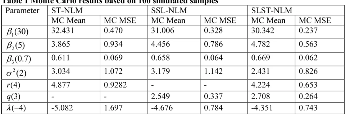
The result of simulation study for ST, SSL and SLST random error distributions with estimated MSE and Mean are given in Table 1. In this table the true values have been put in to the parenthesis, MC Mean has been calculated according to 100

1ˆ 100kj j



and MC MSE which has been determined by 100 2

1(ˆkj k) 100

j  



is the empirical mean squared error. In the indicated formula ˆ_k is the estimated parameter of true parameter



_k.

The values in Table 1 indicated that the MC MSE for model parameters are smaller in SLST model than ST and SSL models. Thus SLST-NLM would be better fitted rather than ST-NLM and SSL-NLM for nonsymmetrical data.

This statement has been approved by the values in Table 2. In this table the arithmetic average of the measurements for comparing the models (DIC, EAIC, EBIC, B) are given. These measurements would be smaller in SLST-NLM than the mentioned models. Thus, this particular model has better fitted than the competitor models.

Table 1 Monte Carlo results based on 100 simulated samples

Parameter ST-NLM SSL-NLM SLST-NLM

MC Mean MC MSE MC Mean MC MSE MC Mean MC MSE

1(30)



32.431 0.470 31.006 0.328 30.342 0.237 2(5)



3.865 0.934 4.456 0.786 4.782 0.563 3(0.7)



0.611 0.069 0.658 0.064 0.669 0.062 2₍₂₎



3.034 1.072 3.179 1.142 2.431 0.826 (4) r 4.877 0.9282 - - 4.224 0.653 (3) q - - 2.549 0.337 2.708 0.264 ( 4)   -5.082 1.697 -4.676 0.784 -4.351 0.743

Table 2 Comparison between ST-NLM , SSL-NLM and SLST-NLM fitting by using different Bayesian criteria

Model Criterion

MC DIC MC EAIC MC EBIC MC B

ST 138.485 88.977 87.173 -376.067

SSL 135.955 82.918 81.114 -373.054

Special Issue on New Dimensions in Economics, Accounting and Management

Openly accessible at http://www.european-science.com 238 Real Data

We use a Bayesian analysis of the ultrasonic calibration data, which has been described in Lin et al. (2007) and Lachos et. al. (2011), to investigate our method. These data are generated from National institutes of Standards and Technology (NIST) study by Chwirut (1979) involving ultrasonic calibration, where the response variableyand the predictor variable is metal distancex.

The data consists of 214observations and is available freely in the R package Nlsmsn. We consider

. . 1 1 2 3 exp( ) , i i d ( , , , , ). i i i i i x Y SLST c q r x  _{    }         (14)

We will use the ST , SSL and SLST distributions to make a comparison.

We consider the following independent priors to apply the Gibbs sampler algorithm: For 1, 2,3

i ,



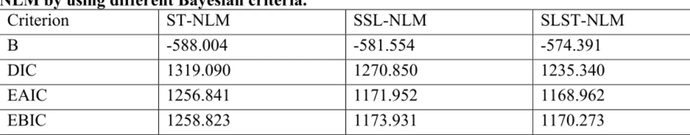
_i N₁(0,1000), N(0,1000),IG(0.01,0.01), ~ exp(0.1)I(2, )r  for skew-t model and ~ exp(0.1)I(2, )q  for SSL model and SLST model. By considering the above priors, we generate two parallel independent runs of the Gibbs sampler chain with size 100,000 for each parameter, for burning in, we exclude the first 10000 iterations. Also to avoid correlation problem we consider thin size 10, hence, the effective sample size are 9000. For each sample the posterior mean of the parameter and the DIC, EAIC, BIC and B are calculated.

Posterior mean and standard deviation of parameter under the distributions ST, SSL and SLST have been demonstrated in Table 3. Also, in Table 4 the values of model selection criteria are given. From this table we see that the SLST-NLM has a better fit to this data than ST-NLM and SSL-NLM.

Table 3 Ultrasonic calibration data set. Summary result from the posterior distribution, Mean and Standard Deviation (SD) for parameter under ST, SSL and SLST distributions

parameter ST-NLM SSL-NLM SLST-NLM

Mean SD Mean SD Mean SD

1



0.1694 0.1165 0.3735 0.0491 0.3899 0.0244

2



0.0059 4.134e-04 0.0091 3.794e-04 0.0073 2.707e-04

3



0.0112 0.00061 0.0082 0.00023 0.0076 0.00012 2  4.4581 1.4371 4.6132 1.4526 2.9144 0.856



0.5360 0.8524 1.2443 0.3304 1.4185 0.3243 r 2.7652 0.5422 - - 2.9288 0.4962 q _{- - 2.1199 0.1861 2.9324 0.1215}

Table 4 Ultrasonic calibration data set. Comparison between ST-NLM, SSL-NLM and SLST-NLM by using different Bayesian criteria.

Criterion ST-NLM SSL-NLM SLST-NLM

B -588.004 -581.554 -574.391

DIC 1319.090 1270.850 1235.340

EAIC 1256.841 1171.952 1168.962

Siavash Pirzadeh Nahooji, Rahman Farnoosh, Nader Nematollahi

Openly accessible at http://www.european-science.com 239 Conclusion

In this paper, we suggest a new nonlinear regression model based on an asymmetric distribution of random error of the model. We employ a MCMC method to obtain the Bayes estimate of the model parameters.

To show the performance of the new model to the existing models, we perform a simulation study. By using B, DIC, EAIC and EBIC criteria, we see that SLNLM has better fit than ST-NLM and SSL-ST-NLM for simulated data and a real data set.

References

Brooks, S.P. (2002). Discussion on the paper by Spiegelhalter, Best, Carlin, and van der Linde. Journal of the Royal Statistical Society. Series B. 64 (3):616-618.

Cancho, V.C., Lachos, V.H., & Ortega, E.M.M. (2010). A nonlinear regression model with skew-normal errors. Statistical Papers. 51:547-558.

Cancho, V. C., Dey, D. K., Lachos, V. H., & Andrade, M. G. (2011). Bayesian nonlinear regression models with scale mixtures of skew-normal distributions: Estimation and case influence diagnostics. Computational Statistics and Data Analysis. 55:588-602.

Carlin, B. P., & Louis, T. A. (2001). Bayes and Empirical Bayes Methods for Data Analysis, 2nd ed. New York, Chapman & Hall.

Chen M. H., Shao Q. M., & Ibrahim, J. (2000). Monte Carlo Methods in Bayesian Computation. New York, Springer-Verlag.

Chwirut D. (1979). Ultrasonic Reference Block Study. Available from: http://www.itl.nist.gov/div898/strd/nls/data/chwirut2.shtml.

Cysneiros, F. J. A., & Vanegas, L. H. (2008). Residuals and their statistical properties in symmetrical nonlinear models. Statistics and Probability Letters. 78:3269-3273.

Cysneiros, F., Cordeiro, G. M., & Cysneiros, A. (2010). Corrected maximum likelihood estimators in heteroscedastic symmetric nonlinear models. Journal of Statistical Computation and Simulation. 80:451-461.

Farnoosh, R., Nematollahi, N., Rahnamaei. Z., & Hajrajabi, A. (2013). A family of skew-slash distributions and estimation of its parameters via an EM Algorithm. Journal of the Iranian Statistical Society. 12(2):271-291.

Garay, A.M, Lachos, V.H., & Abanto-Valle, C. A. (2011). Nonlinear regression models based on scale mixtures of skew-normal distributions. Journal of the Korean Statistical Society. 40:115-124.

Gelfand, A.E, Dey, D. K, & Chang, H. (1992). Model determination using predictive distributions with implementation via sampling-based methods In: Bayesian Statistics. New York, Oxford Univ Press.

Lachos, V.H., Ghosh, P., & Arellano-Valle, R.B. (2010). Likelihood based inference for skew-normal independent linear mixed models. Statistica Sinica. 20:303-322.

Lachos, V.H., Bandyopadhyay, D., & Garay, A.M. (2011) Heteroscedastic nonlinear regression model based on scale mixtures of skew-normal distributions. Statistics and Probability Letters. 81:1208-1217.

Lin, T. I., Lee, J. C., & Hsieh, W. J. (2007). Robust mixture modeling using the skew-t distribution. Statistics and Computing. 17:81-92.

Montenegro, L. C., Lachos, V., & Bolfarine, H. (2009). Local influence analysis of skew-normal linear mixed models. Communications in Statistics. Theory and Methods. 38:484-496.

Special Issue on New Dimensions in Economics, Accounting and Management

Openly accessible at http://www.european-science.com 240 Spiegelhalter, D. J., Best, N. G., Carlin, B. P., & Van Der Linde, A. (2002). Bayesian measures of model complexity and fit. Journal of the Royal Statistical Society. Series B. 64(4):583-639. Xie, F., Lin, J., & Wei, B. (2009a). Diagnostics for skew-normal nonlinear regression models with

AR.1/ errors. Computational Statistics and Data Analysis. 53(12):4403-4416.

Xie, F. C, Wei, B. C., &Lin, J. G., (2009b) Homogeneity diagnostics for skew-normal nonlinear regression models. Statistics and Probability Letters. 79:821-827.