Algorithms for Sparse Signal Recovery in Compressed Sensing

(1)

Aqib Ejaz

School of Electrical Engineering

Thesis submitted for examination for the degree of Master of Science in Technology.

Espoo, 19 May 2015

Thesis supervisor:

Prof. Visa Koivunen Thesis advisor:

(2)

aalto university

school of electrical engineering

abstract of the master’s thesis Author: Aqib Ejaz

Title: Algorithms for Sparse Signal Recovery in Compressed Sensing

Date: 19 May 2015 Language: English Number of pages: 9+65

Department of Signal Processing and Acoustics Professorship: Signal Processing

Supervisor: Prof. Visa Koivunen Advisor: D.Sc. (Tech.) Esa Ollila

Compressed sensing and sparse signal modeling have attracted considerable re-search interest in recent years. The basic idea of compressed sensing is that by exploiting the sparsity of a signal one can accurately represent the signal using fewer samples than those required with traditional sampling. This thesis reviews the fundamental theoretical results in compressed sensing regarding the required number of measurements and the structure of the measurement system. The main focus of this thesis is on algorithms that accurately recover the original sparse signal from its compressed set of measurements. A number of greedy algorithms for sparse signal recovery are reviewed and numerically evaluated. Convergence properties and error bounds of some of these algorithms are also reviewed. The greedy approach to sparse signal recovery is further extended to multichannel sparse signal model. A widely-used non-Bayesian greedy algorithm for the joint recovery of multichannel sparse signals is reviewed. In cases where accurate prior information about the unknown sparse signals is available, Bayesian estimators are expected to outperform non-Bayesian estimators. A Bayesian minimum mean-squared error (MMSE) estimator of the multichannel sparse signals with Gaussian prior is derived in closed-form. Since computing the exact MMSE estimator is infeasible due to its combinatorial complexity, a novel algorithm for approximating the multichannel MMSE estimator is developed in this thesis. In comparison to the widely-used non-Bayesian algorithm, the developed Bayesian algorithm shows better performance in terms of mean-squared error and probability of exact support recovery. The algorithm is applied to direction-of-arrival estimation with sensor arrays and image denoising, and is shown to provide accurate results in these applications.

Keywords: compressed sensing, sparse modeling, greedy algorithms, MMSE, Bayesian, multichannel sparse recovery.

(3)

The work I have presented in this thesis was carried out at the Department of Signal Processing& Acoustics, Aalto University during a period of eight months starting in June of 2014. The aim of this work was to develop a solid understanding of compressed sensing that would result in an original contribution to this rapidly growing field. This involved a lot of literature review and computer simulations. The final outcome of all that hard work is RandSOMP, a novel Bayesian algorithm developed in this thesis for recovering multichannel sparse signals in compressed sensing.

This work would not be possible without the continuous help and guidance that I received from my supervisor, Prof. Visa Koivunen, and my advisor, D.Sc. (Tech) Esa Ollila. I thank them for trusting in my abilities and giving me the opportunity to work in their research group. I owe special thanks to Esa Ollila for his deep involvement with this work. His insightful research ideas and helpful comments have mainly guided the course of this work.

Finally, I would like to thank my family and friends for their love and support. Your presence makes my life richer.

Otaniemi, 19 May 2015

Aqib Ejaz

(4)

Symbols

m A scalar x A vector A A matrix xT _{Transpose of} _x xH _{Conjugate transpose of} _x

Rn The n-dimensional real vector space Cn The n-dimensional complex vector space

k · k0 `0-pseudonorm

k · k1 `1-norm

k · k2 Euclidean norm

k · kF Frobenius norm

⊗ Kronecker product

vec(·) Vectorization operation

E[·] Expected value

Tr(·) Trace of a square matrix

(7)

CoSaMP Compressive sampling matching pursuit

DOA Direction-of-arrival

FBMP Fast Bayesian matching pursuit

IHT Iterative hard thresholding

MMSE Minimum mean-squared error

MMV Multiple measurement vectors

MSE Mean-squared error

MUSIC Multiple signal classification

NSP Null space property

OMP Orthogonal matching pursuit

PER Probability of exact support recovery

PSNR Peak signal-to-noise ratio

RandCoSaMP Randomized compressive sampling matching pursuit RandIHT Randomized iterative hard thresholding

RandOMP Randomized orthogonal matching pursuit

RandSOMP Randomized simultaneous orthogonal matching pursuit

RIP Restricted isometry property

RMSE Root mean-squared error

SMV Single measurement vector

SNR Signal-to-noise ratio

SOMP Simultaneous orthogonal matching pursuit

ULA Uniform linear array

WRS Weighted random sampling

(8)

List of Figures

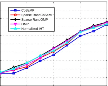
2.1 Unit Balls in_R2 . . . 6 4.1 Fractional size of the correctly identified support vs SNR. The

pa-rameter values are: k = 20, m = 150, n = 300, L = 10. For the given settings, there is not much difference in the performance of these algorithms. However, Sparse RandOMP seems to be slightly better than the rest of the algorithms. . . 33 4.2 Fractional size of the correctly identified support vs SNR. The

param-eter values are: k = 50, m = 150, n = 300, L = 10. The difference in performance of these algorithms is more noticeable in this case. Sparse RandOMP is clearly the best performing algorithm. On the other hand, CoSaMP lags far behind the rest of the algorithms. . . . 33 4.3 Mean-squared error vs SNR. The parameter values are: k = 20,

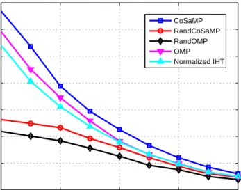
m = 150, n = 300, L = 10. Bayesian algorithms (RandOMP and RandCoSaMP) have lower mean-squared error than non-Bayesian algorithms. . . 34 4.4 Mean-squared error vs SNR. The parameter values are: k = 50,

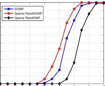
m = 150, n = 300, L = 10. Bayesian algorithms (RandOMP and RandCoSaMP) have lower mean-squared error than non-Bayesian algorithms. . . 34 5.1 Probability of exact support recovery vs SNR. The parameter values

are: m= 150, n= 300, k = 20,L= 10, q= 30. Sparse RandSOMP provides higher probability of exact support recovery than both SOMP and Sparse RandOMP. . . 45 5.2 Relative mean-squared error vs SNR. The parameter values are:

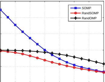
m = 150, n = 300, k = 20, L = 10, q = 30. RandSOMP provides lower MSE than both SOMP and RandOMP. . . 46 5.3 Probability of exact support recovery vs number of measurement

vectors (q). The parameter values are: m = 150, n = 300, k = 20,

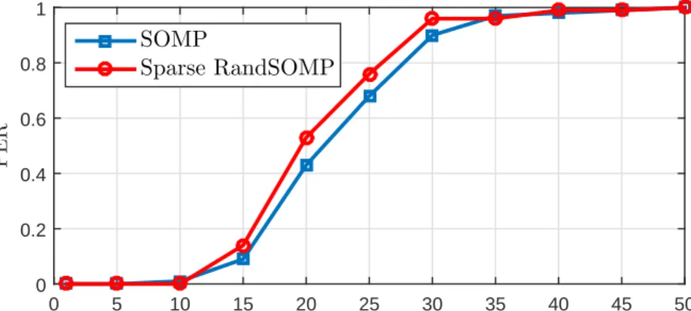
L= 10, SNR= 5dB. Sparse RandSOMP provides higher probability of exact support recovery than SOMP. . . 46 6.1 PER rates vs SNR. The parameter values are: m = 150, n = 300,

k= 20, L= 15, q= 30. Sparse RandSOMP has higher PER rates for all the given SNR levels. . . 52

(9)

6.2 Normalized MSE vs SNR. The parameter values are: m = 150,

n= 300, k= 20, L= 15, q= 30. RandSOMP has lower normalized MSE for all the given SNR levels. . . 52 6.3 PER rates vsq. The parameter values are: m = 150,n = 300,k = 20,

L= 15, SNR= 3 dB. Sparse RandSOMP has higher PER rates for all the given values ofq. . . 53 7.1 Relative frequency vs DOA (degrees). The parameter values are:

m= 20, n = 90, q= 50,k = 2, L= 10, SNR =−5dB, true DOAs at

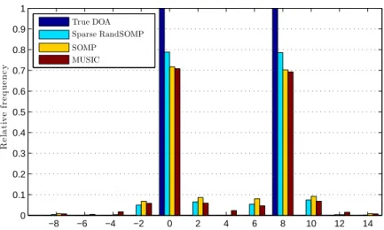
0◦ and 8◦. Each algorithm has correctly estimated the true DOAs in every trial. . . 55 7.2 Relative frequency vs DOA (degrees). The parameter values are:

m= 20, n= 90, q= 50, k = 2,L= 10, SNR=−15 dB, true DOAs at0◦ and 8◦. Sparse RandSOMP has correctly found the true DOAs more frequently than SOMP and MUSIC. . . 56 7.3 Relative frequency vs DOA (degrees). The parameter values are:

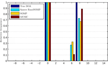
m= 20, n = 90, q= 50,k = 2, L= 10, SNR =−5dB, true DOAs at

0◦ and 7.2◦. The source at 7.2◦ is incorrectly located more frequently at8◦ and less frequently at 6◦. . . 57 7.4 Two overlapping patches (black and gray) shown within a larger RGB

image. . . 58 7.5 RGB image denoising with SOMP and RandSOMP (L= 10,C = 0.99).

(a) Original image; (b) Noisy image (PSNR = 12 dB); (c) Denoised image with SOMP (PSNR = 22.57 dB); (d) Denoised image with RandSOMP (PSNR= 22.47dB). . . 59

(10)

Chapter 1 Introduction

1.1 Background

In signal processing, the Nyquist-Shannon sampling theorem has long been seen as the guiding principle for signal acquisition. The theorem states that an analog signal can be perfectly reconstructed from its samples if the samples are taken at a rate at least twice the bandwidth of the signal. This gives a sampling rate which is sufficient to reconstruct an analog signal from its samples. But is this sampling rate necessary as well? The recently developed field of compressed sensing [1, 2, 3, 4, 5] has successfully answered that question. It turns out that it is possible to sample a signal at a lower than Nyquist rate without any significant loss of information. In order to understand when and how this is possible, let us start with an example.

Consider a digital camera that acquires images with a 20 megapixel resolution. A raw image produced by this camera would require about 60 megabytes (MB) of storage space. Typically, images are compressed using some compression technique (e.g., JPEG standard) which often results in a large reduction in the size of the image. The same 60 MB raw image, for example, could be compressed and stored in a 600 kilobytes storage space without any significant loss of information. The key fact that enables this compression is the redundancy of information in the image. If one could exploit this information redundancy then it should be possible to sample at a lower rate. The real challenge here is to know what is important in a signal before the signal is even sampled. The theory of compressed sensing provides a surprising solution to that challenge, i.e., the solution lies in the randomly weighted sums of signal measurements.

In compressed sensing, the signal to be sampled is generally represented as a vector, sayx∈_Rn_{. The information contained in}_x_{is assumed to be highly redundant.} This means xcan be represented in an orthonormal basis system W∈_Rn×n _using

k n basis vectors, i.e., x=Ws. The vector s∈_Rn _{has only} _k _{non-zero elements} and is called the sparse representation ofx. A linear sampling process is represented by a measurement matrix A∈_Rm×n_{. The sampled signal is represented as a vector} y = Ax+v, where y ∈ _Rm _and _v _∈

Rm represents additive noise in the system.

The goal in compressed sensing is to acquire the signalx with no or insignificant loss of information using fewer than n measurements, i.e., to accurately recover x from

(11)

y with m < n. In other words, the central theme of compressed sensing is about finding a sparse solution to an underdetermined linear system of equations.

A fundamental question in compressed sensing is about how small the number of measurementsm can be made in relation to the dimension n of the signal. The role played in the sampling process by the sparsity k of the signal is also worth exploring. Theoretical results in compressed sensing prove that the minimum number of measurementsmneeded to capture all the important information in a sparse signal grows linearly with k and only logarithmically with n [2]. This makes sense since the actual amount of information in the original signal is indicated byk and not by

n, which is why m has a stronger linear dependence on k but a weaker logarithmic dependence onn.

The design of the measurement matrixAis also an important aspect of compressed sensing. It is desired that A is not dependent on the signal being sampled so that it can be applied to any sparse signal regardless of the actual contents of the signal. As it turns out, A can be chosen independent of the sampled signal as long as it is different from the basisW in which the signal is known to be sparse. Theoretical results in compressed sensing have shown that random matrices that possess the restricted isometry property and/or have low mutual coherence among their columns are suitable candidates for this purpose [1, 2].

The recovery of the signalx(or equivalentlys) from its compressed measurements yhas gained a lot of attention in the past several years. A number of techniques have been developed for this purpose. These can be broadly classified into two categories. First of these is the set of techniques that are based on `1-norm minimization using

convex optimization [6, 7, 8]. These techniques generally have excellent recovery performance and also have guaranteed performance bounds. High computational cost is one major drawback of these techniques, which makes it difficult to apply these techniques to large-scale problems. Alternative techniques include iterative greedy methods [9, 10, 11, 12]. These methods make sub-optimal greedy choices in each iteration and hence are computationally much more efficient. They may suffer a little in their recovery performance but are much more useful in large-scale problems. These methods generally have proven performance bounds, making them a reliable set of tools for sparse signal recovery.

1.2 Research Problem

The main focus of this thesis is the study of signal recovery algorithms in compressed sensing. Specifically, greedy algorithms that estimate the sparse signals in both Bayesian and non-Bayesian frameworks are considered in this thesis. The objective is to give a performance evaluation of several greedy algorithms under different parameter settings. Multichannel sparse signal recovery problem is also considered and a novel Bayesian algorithm is developed for solving this problem.

(12)

3

1.3 Contributions of the Thesis

The following are the main contributions of this thesis:

• Several existing theoretical results regarding the measurement system and the recovery algorithms in compressed sensing are reviewed in detail in Chapters 2-3. This includes the results on the minimum number of measurements required for accurate signal recovery, structure of the measurement matrix, and error bounds of some of the recovery algorithms.

• Several greedy algorithms for sparse signal recovery are reviewed in Chapters 3-4 and their codes are developed in Matlab. Based on simulations carried out in Matlab, the signal recovery performance of these algorithms is numerically evaluated and compared.

• A novel Bayesian algorithm for multichannel sparse signal recovery is developed as the main contribution of this thesis in Chapter 5. A generalization of the developed algorithm for complex-valued signals is developed in Chapter 6. The performance of the algorithm is numerically evaluated in Matlab. The algorithm is applied to direction-of-arrival (DOA) estimation with sensor arrays and image denoising, and is shown to produce accurate results in these applications. The algorithm and its derivation are also described in a conference paper that has been submitted for publication [13].

1.4 Outline of the Thesis

The thesis is organized into eight chapters. An introduction to this thesis is given in Chapter 1. In Chapter 2, we present several basic definitions. Some fundamental theoretical results in compressed sensing are also presented. Chapter 3 reviews some of the commonly used greedy algorithms for signal recovery in compressed sensing. In Chapter 4, we review several Bayesian algorithms that take prior knowledge about the sparse signal into account. We numerically evaluate signal recovery performance of several Bayesian and non-Bayesian methods in this chapter. In Chapter 5, we present the problem of multichannel sparse signal recovery and develop a novel Bayesian algorithm for solving it. The performance of the developed algorithm is numerically evaluated and compared with a widely-used greedy algorithm. Chapter 6 generalizes the developed algorithm for recovering multichannel complex-valued sparse signals. In Chapter 7, we apply the algorithms for multichannel sparse signal recovery in DOA estimation with sensor arrays and image denoising. Concluding remarks of the thesis are given in Chapter 8.

(13)

Compressed Sensing

In this chapter we will formulate the problem of sparse signal recovery in compressed sensing. We will give several basic definitions. We will also review important theoret-ical results in compressed sensing concerning the minimum number of measurements required for accurate signal recovery and the structure of the measurement matrix. We start the chapter with a formal mathematical formulation of the compressed sensing model.

Let x ∈_Rn _{be an unknown signal vector. The vector} _x _{can be assumed to be} sparse (i.e., most of the entries are zero) either in the canonical basis or some other non-canonical orthonormal basis. For simplicity of representation, xis assumed to be sparse in the canonical basis. Let A ∈_Rm×n _{be a known measurement matrix} with m < n. Observed vectory∈_Rm _{is then modeled as}

y=Ax. (2.1)

It is then required to recover x given the knowledge of just A and y. Since it is assumed that A has fewer rows than columns (underdetermined system), dimension of the null space ofAwill be greater than zero (N ullSpace(A) ={z∈_Rn_:_Az₌₀_}). As a consequence, the mapping from xto yis non-injective since for every xthere are infinitely many vectors of the form x+z (z ∈ N ullSpace(A)\{0}) such that A(x+z) =y. Therefore, in general, it is not possible to recoverxfromyunless there are additional conditions which are satisfied by x. Sparsity is one such condition. In practice, most of the natural signals are either sparse or well approximated by sparse signals. Formally, a vector is said to be k-sparse if at most k of its components are non-zero. When xis known to be sparse then it becomes possible to recover it in an underdetermined framework. Besides sparsity ofx, the structure of the measurement matrixA is also crucial for accurate recovery. This will be discussed in greater detail later on, but first we introduce basic terminology.

Definition 1. Cardinality of a finite set S is defined as ‘the number of elements of the set’. Cardinality of S is indicated by |S|.

Definition 2. For a real number p≥1, `p-norm of a vector x∈Rn is defined as kxkp := n X i=1 |xi|p !1/p , 4

(14)

5

where |xi| indicates the absolute value of the i-th component of x. Two commonly used `p-norms are the `1-norm and the `2-norm:

kxk1 := n X i=1 |xi|, kxk2 := v u u t n X i=1 |xi|2.

For 0< p <1, `p-norm as defined above does not satisfy the triangle inequality and therefore cannot be called a norm. Instead it is called a quasinorm as it satisfies the following weaker version of the triangle inequality,

kx+ykp ≤c(kxkp+kykp), with c= 21/p−1_.

Definition 3. The `0-pseudonorm of a vector x∈Rn is defined as

kxk0 := {j :xj 6= 0} ,

i.e., the `0-pseudonorm of a vector is defined as the number of non-zero components

of the vector.

The `0-pseudonorm is not a proper norm as it does not satisfy the homogeneity

property, i.e.,

kcxk0 6=|c|kxk0,

for all scalarsc6=±1. The `0-pseudonorm and `p-norm with three different values of

pare illustrated in Figure 2.1.

Definition 4. Spark of a matrix A ∈ _Rm×n _{is defined as ‘the cardinality of the}

smallest set of linearly dependent columns of A’, i.e.,

Spark(A) = min |V| such that V ⊆[n] and rank(AV)<|V|,

where [n] = {1,2, . . . , n} and AV is the matrix consisting of those columns of A

which are indexed by V.

For a matrix A∈_Rm×n_{, every set of} _m_{+ 1} _{columns of} _A _{is guaranteed to have} linearly dependent columns. On the other hand, one needs to take at least two column vectors to form a linearly dependent set. Therefore, 2≤Spark(A)≤m+ 1. The definition of the spark of a matrix draws some parallels to the definition of the rank of a matrix, i.e., spark is the cardinality of the smallest set of linearly dependent columns whereas rank is the cardinality of the largest set of linearly independent columns. While rank of a matrix can be computed efficiently, computing spark of a matrix is NP-Hard [14].

(15)

(a)kxk₂ = 1 (b)kxk₁ = 1

(c)kxk₁_/₂ = 1 (d)kxk₀ = 1 Figure 2.1: Unit Balls in _R2

From the definition of the spark of a matrix A, it can be concluded that kzk0 ≥

Spark(A)for all z∈N ullSpace(A)\{0}. Now suppose that xis k-sparse and A is designed so that Spark(A)≥2k+ 1. Then by solving the optimization problem,

min kxk0 subject to Ax=y, (P0)

one is guaranteed to recoverxexactly. It is quite easy to show that above formulation indeed recovers x unambiguously. Since kxk0 ≤ k and kzk0 ≥ Spark(A)≥ 2k+ 1

for all z ∈ N ullSpace(A)\{0} it follows that kx + zk0 ≥ k + 1 and therefore

kxk0 <kx+zk0. In other words, xis sparser than all other solutions (x+z) of (2.1)

and thus solving (P0) will recover xand not any other solution.

So far it has been assumed that there was no noise present in the system which is not a realistic assumption when real-world data or physical observations are processed. A more realistic model in which the observations are contaminated by an additive noise is given as

(16)

7 where v∈_Rm _{is the unknown noise vector. To compensate for the effect of noise in} (2.2) the optimization problem (P0) is slightly modified as

min kxk0 subject to ky−Axk2 ≤η, (P0,η) whereη is a measure of the noise power. In (P0,η) the objective is to find the sparsest vector x such that`2-norm of the error y−Ax remains within a certain bound η.

Minimizing `0-pseudonorm leads to exact recovery in noiseless case (provided A

is appropriately chosen) but this approach suffers from one major drawback. It turns out that both (P0) and (P0,η) are NP-hard problems [15] so in general there is no known algorithm which can give a solution to these problems in polynomial time and exhaustive search is the only option available which is not practical even in fairly simple cases.

To circumvent this limitation several approaches have been proposed in the literature. One such popular approach is to solve the optimization problems in which

`1-norm replaces the `0-pseudonorm, i.e.

min kxk1 subject to Ax=y, (P1)

min kxk1 subject to ky−Axk2 ≤η. (P1,η) (P1) is referred to as basis pursuit while (P1,η) is known as quadratically-constrained

basis pursuit [7]. Since these are convex optimization problems, there are methods that can efficiently solve them. The only question that remains is whether the solution obtained through`1-minimization is relevant to the original`0-minimization problem

and the answer to that is in the affirmative. In fact, ifA satisfies the so-called null space property (NSP) [16] then solving (P1) will recover the same solution as the one obtained by solving (P0).

Definition 5. Anm×n matrixAis said to satisfy the null space property of orderk if the following holds for all z∈N ullSpace(A)\{0} and for all S⊂[n] ={1,2, . . . , n}

with |S|=k,

kzSk1 <kzSk1,

where zS is the vector consisting of only those components of z which are indexed by

S while z_S is the vector consisting of only those components of z which are indexed by S = [n]\S.

If a matrix A satisfies NSP of order k then it is quite easy to see that for every k-sparse vector x and for every z∈N ullSpace(A)\{0} it holds that kxk1 <

kx+zk1. This means that the k-sparse solutionx to (2.1) will have smaller`1-norm

than all other solutions of the form(x+z) and therefore by solving (P1) one will recover x unambiguously. Furthermore, if a matrix satisfies NSP of order k then it implies that the spark of the matrix will be greater than 2k. Therefore it is very important that the measurement matrix satisfies NSP. It turns out that there exists an effective methodology that generates measurement matrices which satisfy NSP. Before proceeding, it is important to first introduce the concept ofrestricted isometry property (RIP) [3, 17].

(17)

Definition 6. An m×n matrix A is said to satisfy the restricted isometry property of order 2k if the following holds for all 2k-sparse vectors x with 0< δ2k <1,

(1−δ2k)kxk22 ≤ kAxk 2

2 ≤(1 +δ2k)kxk22,

where δ2k is called the restricted isometry constant.

A matrix that satisfies RIP of order 2k will operate on k-sparse vectors in a special way. Consider twok-sparse vectors x1 and x2 and a measurement matrixA

that satisfies RIP of order2k. Nowx₁−x₂ will be2k-sparse and since Ais assumed to satisfy RIP of order 2k the following will hold,

(1−δ2k)kx1−x2k22 ≤ kA(x1 −x2)k22 ≤(1 +δ2k)kx1 −x2k22,

⇒(1−δ2k)kx1−x2k22 ≤ kAx1−Ax2k22 ≤(1 +δ2k)kx1−x2k22.

This means that the distance between Ax1 and Ax2 is more or less the same as

the distance between x1 and x2, which implies that no two distinct k-sparse vectors

are mapped by A to the same point. As a consequence, it can be argued that RIP of order 2k implies that the spark of the matrix is greater than 2k. Furthermore, it can be proved that RIP of order 2k with 0 < δ2k < 1/(1 +

√

2) implies NSP of order k [18]. Therefore for accurate recovery of sparse signals it is sufficient that the measurement matrix satisfies RIP. Theoretical results in compressed sensing show that anm×n matrix will satisfy RIP fork-sparse vectors with a reasonably high probability if, m =O klogn k ,

and entries of the matrix are taken independent of each other from a Gaussian or a Bernoulli distribution [19]. This gives a simple but effective method of constructing measurement matrices that enable accurate recovery of sparse signals.

In addition to `1-minimization, there exist greedy methods for sparse signal

recovery in compressed sensing. Greedy pursuit methods and thresholding-based methods are two broad classes of these algorithms which are generally faster to compute than`1-minimization methods. Orthogonal matching pursuit (OMP) [9, 10]

andcompressive sampling matching pursuit (CoSaMP) [12] are two of the well-known greedy pursuit methods whereas iterative hard thresholding (IHT) and its many variants [11, 20, 21] are examples of thresholding-based methods. Some of these algorithms are discussed in detail in the next chapter.

(18)

Chapter 3 Non-Bayesian Greedy Methods

Sparse signal recovery based on `1-minimization is an effective methodology which,

under certain conditions, can result in an exact signal recovery. In addition, `1

-minimization also has very good performance guarantees which make it a reliable tool for sparse signal recovery. One drawback of the methods based on`1-minimization

is their higher computational cost in large-scale problems. Therefore, algorithms that scale up better and are similar in performance in comparison to the convex optimization methods are needed. Greedy algorithms described in this chapter are good examples of such methods [9, 10, 11, 12, 20, 21]. These algorithms make significant savings in computation by performing locally optimal greedy iterations. Some of these methods also have certain performance guarantees that are somewhat similar to the guarantees for `1-minimization. All of this makes greedy algorithms

an important set of tools for recovering sparse signals.

The greedy algorithms reviewed in this chapter recover the unknown sparse vector in a non-Bayesian framework, i.e., the sparse vector is treated as a fixed unknown and no prior assumption is made about the probability distribution of the sparse vector. In contrast, the Bayesian methods [22, 23, 24] reviewed in Chapter 4 consider the unknown sparse vector to be random and assume that some prior knowledge of the signal distribution is available. Non-Bayesian greedy methods are computationally very simple. There are also some theoretical results associated with non-Bayesian greedy methods that provide useful guarantees regarding the convergence and error bounds of these methods.

Bayesian methods do not have any theoretical guarantees regarding their recovery performance. They also require some kind of greedy approximation scheme to circumvent their combinatorial complexity. Their use for sparse signal recovery is justified only when some accurate prior knowledge of the signal distribution is available. In such cases, Bayesian methods can incorporate the prior knowledge of the signal distribution into the estimation process and hence provide better recovery performance than non-Bayesian methods.

(19)

3.1 Orthogonal Matching Pursuit

Consider a slightly modified version of the optimization problem (P0,η) in which role of the objective function is interchanged with the constraint function, i.e.,

min ky−Axk2

2 subject to kxk0 ≤k. (P2)

In (P2) the objective is to minimize the squared`2-norm of the residual errory−Ax

subject to the constraint that xshould be k-sparse. Let us definesupport set of a vector x asthe set of those indices where x has non-zero components, i.e.,

supp(x) ={j :xj 6= 0},

where xj denotes j-th component of x. Assuming A∈Rm×n and x∈Rn, the total

number of different supports thatk-sparse xcan have is given by L=Pk

i=1

_n i

. In theory one could solve (P2) by going through all L supports one by one and for each support finding the optimal solution by projecting yonto the space spanned by those columns of A which are indexed by the selected support. This is equivalent to solving a least squares problem for each possible support of x. Finally one could compare allLsolutions and select the one that gives the smallest squared `2-norm of

the residual. Although least squares problem can be solved efficiently, difficulty with the given brute-force approach is that L is a huge number even for fairly small-sized problems and computationally it is not feasible to go through all of theL supports.

Orthogonal matching pursuit (OMP) [9, 10] is a greedy algorithm which overcomes this difficulty in a very simple iterative fashion. Instead of projectingyontoLdifferent subspaces (brute-force approach), OMP makes projections onto n columns of A. In comparison toL,nis a much smaller number and therefore computational complexity of OMP remains small. In each iteration, OMP projects the current residual error vector onto all n columns of A and selects that column which gives smallest`2-norm

of the projection error. Residual error for next iteration is then computed by taking the difference betweeny and its orthogonal projection onto the subspace spanned by all the columns selected up to the current iteration. Afterk iterations OMP gives a set ofk ‘best’ columns of A. Thesek columns form an overdetermined system of equations and an estimate of xis obtained by solving that overdetermined system for observed vector y. A formal definition of OMP is given in Algorithm 1.

In the above algorithm, the iteration number is denoted by a superscript in parenthesis, e.g., S(i) _{denotes the support set}_S _at_i_{-th iteration, while}_a

j denotes the

j-th column of A. In line 4, r denotes the residual error vector while aT

j r/aTjaj

aj in line 5 is the orthogonal projection ofr onto aj and thereforer−

aT

j r/ajTaj

aj is the projection error ofr with aj. The solution of the optimization problem in line 7 can be obtained by solving an overdetermined linear system of equations. If S(i)

indexed columns of A are linearly independent then the non-zero entries of xb

(i) _can

be computed as linear least squares (LS) solution:

b x(_Si()i) = AT_S(i)A_S(i) −1 AT_S(i)y,

(20)

11

Algorithm 1: Orthogonal Matching Pursuit (OMP) [9], [10]

1 Input: Measurement matrixA∈_Rm×n, observed vectory∈_Rm, sparsity k 2 Initialize: S(0)←_∅, x_b(0) ←0 3 for i←1 to k do 4 r←y−Axb (i−1) 5 bj ←argmin j∈[n] r− aT jr/aTjaj aj 2 2 6 S(i) ←S(i−1)∪ n b jo 7 xb (i) _←_argmin e x∈Rn ky−Axek 2 2 s.t. supp(xe)⊆S (i) 8 end

9 Output: Sparse vector xis estimated as xb =xb

(k)

where A_S(i) is an m×i matrix that consists of only S(i) indexed columns of A and

b

x_S(i()i) is an i×1vector that represents non-zero entries of xb

(i)_.

OMP greedily builds up support of the unknown sparse vector one column at a time and thereby avoids large combinatorial computations of the brute-force method. There are also some theoretical results which give recovery guarantees of OMP for sparse signals. Although the performance guaranteed by these results is not as good as those for `1-based basis pursuit, they nevertheless provide necessary theoretical

guarantees for OMP which is otherwise a somewhat heuristic method. One such result states that in the absence of measurement noise OMP will succeed in recovering an arbitrary k-sparse vector ink iterations with high probability if entries of them×n

measurement matrix are Gaussian or Bernoulli distributed and m=O(klogn) [25]. This result does not mean that OMP will succeed in recovering all k-sparse vectors under the given conditions, i.e., if one tries to recover different k-sparse vectors one by one with the same measurement matrix then at some point OMP will fail to recover some particulark-sparse vector. In order to guarantee recovery of allk-sparse vectors, OMP needs to have more measurements, i.e. m =O(k2logn)[26]. If OMP is allowed to run for more thank iterations then the number of measurements needed for guaranteed recovery can be further reduced from O(k2_log_n₎_[27].

3.2 Compressive Sampling Matching Pursuit

Compressive sampling matching pursuit (CoSaMP) [12] is an iterative greedy algo-rithm for sparse signal recovery. The main theme of CoSaMP is somewhat similar to that of orthogonal matching pursuit (OMP), i.e., each iteration of CoSaMP involves both correlating the residual error vector with the columns of the measurement matrix and solving a least squares problem for the selected columns. CoSaMP also has a guaranteed upper bound on its error which makes it a much more reliable tool for sparse signal recovery.

A formal definition of CoSaMP is given in Algorithm 2. In each iteration of CoSaMP, one correlates the residual error vector r with the columns of the

(21)

Algorithm 2: Compressive Sampling Matching Pursuit (CoSaMP) [12]

1 Input: Measurement matrixA∈_Rm×n, observed vectory∈_Rm, sparsity k 2 Initialize: S(0)←_∅, x_b(0) ←0, i←1

3 while stopping criterion is not met do 4 r←y−Axb (i−1) 5 Se(i) ←S(i−1)∪supp H2k(ATr) 6 xe (i) _←_argmin z∈Rn ky−Azk2 2 s.t. supp(z)⊆Se(i) 7 xb (i) _←_H k(xe (i)₎ 8 S(i) ←supp(xb (i)₎ 9 i←i+ 1 10 end

(i) _{from the last iteration}

measurement matrix A. One then selects 2k columns of A corresponding to the 2k

largest absolute values of the correlation vectorATr, where k denotes the sparsity of the unknown vector. This selection is represented by supp(H2k(ATr)) in line 5 of Algorithm 2. H2k(.)denotes the hard thresholding operator. Its output vector is obtained by setting all but the largest (in magnitude) 2k elements of its input vector to zero. The indices of the selected columns (2k in total) are then added to the current estimate of the support (of cardinalityk) of the unknown vector. A3k-sparse estimate of the unknown vector is then obtained by solving the least squares problem given in line 6 of Algorithm 2. The hard thresholding operatorHk(.) is applied on the3k-sparse vector to obtain thek-sparse estimate of the unknown vector. This is a crucial step which ensures that the estimate of the unknown vector remains k-sparse. It also makes it possible to get rid of any columns that do not correspond to the true signal support but which might have been selected by mistake in the correlation step (line 5). This is a unique feature of CoSaMP which is missing in OMP. In OMP, if a mistake is made in selecting a column then the index of the selected column remains in the final estimate of the signal support and there is no way of removing it from the estimated support. In contrast, CoSaMP is more robust in dealing with the mistakes made in the estimation of the signal support.

The stopping criterion for CoSaMP can be set in a number of different ways. One way could be to run CoSaMP for a fixed number of iterations. Another possible way is to stop running CoSaMP once the `2-norm of the residual error vector r becomes

smaller than a predefined threshold. The exact choice of a stopping criterion is often guided by practical considerations.

The computational complexity of CoSaMP is primarily dependent upon the complexity of solving the least squares problem in line 6 of Algorithm 2. The authors of CoSaMP suggest in [12] that the least squares problem should be solved iteratively using either Richardson’s iteration [28, Section 7.2.3] or conjugate gradient [28, Section 7.4]. The authors of CoSaMP have also analyzed the error performance of these iterative methods in the context of CoSaMP. It turns out that the error decays

(22)

13 exponentially with each passing iteration, which means that in practice only a few iterations are enough to solve the least squares problem.

3.2.1 Error bound of CoSaMP

Letx∈_Rn _{be an arbitrary vector and} _x

k be the best k-sparse approximation ofx, i.e. amongst all k-sparse vectors,xk is the one which is nearest (under any `p-metric) tox. Furthermore let xbe measured according to (2.2), i.e.,

y=Ax+v,

where A∈_Rm×n _{is the measurement matrix and} _v_{is the noise vector. Now if the} following condition holds,

• A satisfies RIP withδ4k≤0.1, then CoSaMP is guaranteed to recover xb

(i) _at _i_{-th iteration such that the error is}

bounded by [12] kx−xb (i)_k 2 ≤ 2−ikxk2 + 20k, where k = kx−xkk2 + 1 √ kkx−xkk1 +kvk2.

This means that the error term 2−ikxk2 decreases with each passing iteration of

CoSaMP and the overall errorkx−xb

(i)_k

2 is mostly determined byk. In case xitself isk-sparse (xk =x) then the error bound of CoSaMP is given by

kx−xb

(i)_k

2 ≤ 2−ikxk2+ 15kvk2.

3.3 Iterative Hard Thresholding

Consider again the optimization problem in (P2). Although the objective function is convex, the sparsity constraint is such that the feasible set is non-convex which makes the optimization problem hard to solve. Ignoring the sparsity constraint for a moment, one way of minimizing the objective function is to use gradient based methods. Iterative hard thresholding (IHT) [20, 11] takes such an approach. In each iteration of IHT the unknown sparse vector is estimated by taking a step in the direction of the negative gradient of the objective function. The estimate obtained this way will not be sparse in general. In order to satisfy the sparsity constraint IHT sets all but the largest (in magnitude) components of the estimated vector to zero using the so-called hard thresholding operator. A formal definition of IHT is given in Algorithm 3 while the objective function used in IHT and its negative gradient are given by J(x) = 1 2ky−Axk 2 2, −∇J(x) =A T₍_y₋_Ax₎ .

(23)

Algorithm 3: Iterative Hard Thresholding (IHT) [20], [11]

1 Input: Measurement matrixA∈_Rm×n, observed vectory∈_Rm, sparsity k 2 Initialize: x_b(0) ←0, i←0

3 while stopping criterion is not met do 4 xe (i+1) _← b x(i)₊_AT₍_y₋_A b x(i)₎ 5 xb (i+1) _←_H k(xe (i+1)₎ 6 i←i+ 1 7 end

(i+1) _{from the last iteration}

In line 5 of the Algorithm 3,Hk(.) denotes the hard thresholding operator. Hk(x) is defined as the vector obtained by setting all but k largest (in magnitude) values of x to zero. Application of hard thresholding operator ensures that the sparsity constraint in (P2) is satisfied in every iteration of IHT. Lastly, IHT cannot run indefinitely so it needs a well defined stopping criterion. There are several possible ways in which a stopping criterion can be defined for IHT. For example, one could limit IHT to run for a fixed number of iterations, or another possibility is to terminate IHT if the estimate of the sparse vector does not change much from one iteration to the next. The choice of a particular stopping criterion is often guided by practical considerations.

Although IHT is seemingly based on an ad hoc construction, there are certain performance guarantees which make IHT a reliable tool for sparse signal recovery. Performance guarantees related to convergence and error bound of IHT are discussed next.

3.3.1 Convergence of IHT

Assuming A∈_Rm×n_{, IHT will converge to a local minimum of (P2) if the following} conditions hold [20],

• rank(A) =m,

• kAk2 <1,

where kAk2 is the operator norm ofA from`2 to `2 which is defined below:

kAk2 := max

kxk2=1

kAxk2.

It can be shown thatkAk2 is equivalent to the largest singular value of A.

3.3.2 Error bound of IHT

Letx∈_Rn _{be an arbitrary vector and} _x

k be the best k-sparse approximation of x. Furthermore let x be measured according to (2.2), i.e.,

(24)

15 where A∈_Rm×n _{is the measurement matrix and} _v_{is the noise vector. Now if the} following condition holds,

• A satisfies RIP withδ3k< √1₃₂,

then IHT is guaranteed to recoverxb

(i) _at_i_{-th iteration such that the error is bounded}

by [11] kx−xb (i)_k 2 ≤ 2−ikxkk2+ 6k, where k = kx−xkk2 + 1 √ kkx−xkk1 +kvk2.

This means that the error term 2−i_k_x

kk2 decreases with each passing iteration of

IHT and the overall error kx−xb

(i)_k

2 is mostly determined by k. In case xitself is

k-sparse (xk=x) then the error bound of IHT is given by kx−xb

(i)_k

2 ≤ 2−ikxk2+ 5kvk2.

3.4 Normalized Iterative Hard Thresholding

The basic version of IHT discussed previously has nice performance guarantees which are valid as long as the underlying assumptions hold. If any one of the underlying assumptions does not hold then the performance of IHT degrades significantly. In particular, IHT is sensitive to scaling of the measurement matrix. This means that even though IHT may converge to a local minimum of (P2) with a measurement matrix satisfying kAk2 < 1, it may fail to converge for some scaling cA of the

measurement matrix for which kcAk2 ≮1. This is clearly an undesirable feature of

IHT. In order to make IHT insensitive to operator norm of the measurement matrix, a slight modification to IHT has been proposed, called the normalized iterative hard thresholding (normalized IHT) [21]. The normalized IHT uses an adaptive step size

(µ) in the gradient update equation of IHT. Any scaling of the measurement matrix is counterbalanced by an inverse scaling of the step size and as a result the algorithm remains stable. A suitable value ofµ, which would ensure that the objective function decreases in each iteration, is then required to be recomputed in each iteration of the normalized IHT. The following discussion describes how µis computed in the normalized IHT.

Let g denote the negative gradient of the objective function J(x) = 1

2ky−Axk 2 2,

i.e.,

g =−∇J(x) = AT(y−Ax).

The gradient update equation for the normalized IHT in i-th iteration is then given by e x(i+1) =xb (i)₊_µ(i)_g(i) =xb (i)₊_µ(i)_AT₍_y₋_A b x(i)).

(25)

An initial guess for the step size µis obtained in a manner similar to the line search method. In the usual line search method, µ would be chosen such that it minimizes the objective function along the straight line in the direction of the negative gradient. For the given (quadratic) objective function this results in the following expression for optimal µ, µ(i) =argmin µ y−A b x(i)+µg(i) 2 2 = g (i)T_g(i) g(i)T_AT_Ag(i).

In case of the normalized IHT, the above value ofµ is not guaranteed to decrease the objective function after the application of the hard thresholding operator (Hk(.)). To ensure that the objective function decreases even after the application of Hk(.),µ is computed using a slightly modified version of the above formula, i.e., it includes the support of the current estimate of the sparse vector as given below:

µ(i) = g (i)T Γ(i)g (i) Γ(i) g(_Γi()iT)A T Γ(i)AΓ(i)g (i) Γ(i) , (3.1) where Γ(i) ₌ _supp₍ b x(i)₎_, _g(i)

Γ(i) is the vector consisting of only those entries of g(i)

which are indexed by Γ(i)_{, and} _A

Γ(i) is the matrix consisting of only those columns

of A which are indexed by Γ(i)_.

The value of µcomputed in (3.1) is only an initial guess. In each iteration of the normalized IHT a move is made in the direction of the negative gradient using this initial guess and the estimate of the sparse vector is updated as

e x(i+1) =xb (i)₊_µ(i)_AT₍_y₋_A b x(i)), b x(i+1) =Hk(xe (i+1)₎_.

If the support of the new estimate xb

(i+1) _{is same as that of the previous estimate}

b

x(i) _{then the initial guess of} _µ_{is guaranteed to decrease the objective function. In}

this case the new estimate of the sparse vector is valid and the algorithm continues to next iteration. When supports of the two estimates are different then in order to guarantee a decrease in the objective function, µneeds to be compared with another parameter ω which is defined as,

ω(i) = (1−c) kbx (i+1)₋ b x(i)_k2 2 kA(xb(i+1)−xb(i))k 2 2 ,

where c is some small fixed constant. Ifµ is less than or equal to ω then µ is still guaranteed to decrease the objective function and there is no need to re-estimate the sparse vector. Otherwise µ is repeatedly scaled down and the sparse vector is re-estimated until µbecomes less than or equal to ω.

Just like in IHT, stopping criterion for the normalized IHT can be based on a fixed number of iterations or on the amount of change in the estimate of the sparse vector from one iteration to another. The stopping criterion can also be based on the norm of the residual error vector. The normalized IHT is formally defined in Algorithm 4.

(26)

17

Algorithm 4: Normalized Iterative Hard Thresholding (Normalized IHT) [21]

1 Input: Measurement matrixA∈_Rm×n, observed vectory∈_Rm, sparsity k,

small constant c, κ >1/(1−c)

2 Initialize: xb

(0) _←₀_, _Γ(0) _←_supp₍_H

k(ATy)),i←0

3 while stopping criterion is not met do 4 g(i)←AT(y−Axb (i)₎ 5 µ(i) ←g(i) T Γ(i)g (i) Γ(i) g(_Γi()iT)AT_Γ(i)AΓ(i)g (i) Γ(i) 6 xe (i+1) _← b x(i)₊_µ(i)_g(i) 7 xb (i+1) _←_H k(xe (i+1)₎ 8 Γ(i+1) ←supp(xb (i+1)₎ 9 if (Γ(i+1) 6= Γ(i)) then 10 ω(i) ←(1−c)kxb (i+1)₋ b x(i)_k2 2 kA(xb (i+1)₋ b x(i)₎_k2 2 11 while (µ(i)> ω(i))do 12 µ(i)←µ(i)/(κ(1−c)) 13 xe (i+1) _← b x(i)+µ(i)g(i) 14 x_b(i+1) ←H_k(x_e(i+1)) 15 ω(i)←(1−c)kxb (i+1)₋ b x(i)_k2 2 kA(xb (i+1)₋ b x(i)₎_k2 2 16 end 17 Γ(i+1) ←supp(x_b(i+1)) 18 end 19 i←i+ 1 20 end

(27)

3.4.1 Convergence of the normalized IHT

Assuming A∈_Rm×n_{, the normalized IHT will converge to a local minimum of (P2)} if the following conditions hold [21],

• rank(A) =m,

• rank(AΓ) =k for all Γ⊂[n]such that|Γ|=k (which is another way of saying

that Spark(A) should be greater than k.)

For the convergence of the normalized IHT, kAk2 is no longer required to be less

than one.

3.4.2 Error bound of the normalized IHT

Error bound of the normalized IHT is obtained using non-symmetric version of restricted isometry property. A matrix A satisfies non-symmetric RIP of order 2k if the following holds for some constants α2k, β2k and for all 2k-sparse vectors x,

α2₂_kkxk2 2 ≤ kAxk 2 2 ≤β 2 2kkxk 2 2.

Let x be an arbitrary unknown vector which is measured under the model given in (2.2). Let xk be the best k-sparse approximation of x. If the normalized IHT computes the step sizeµ in every iteration using (3.1) then let γ2k= (β22k/α22k)−1, otherwise let γ2k = max{1 −(α22k/(κβ22k)),(β22k/α22k)−1}. Now if the following condition holds,

• A satisfies non-symmetric RIP with γ2k<1/8, then the normalized IHT is guaranteed to recover xb

(i) _at _i_{-th iteration such that the}

error is bounded by [21] kx−xb (i)_k 2 ≤ 2−ikxkk2+ 8k, where k = kx−xkk2+ 1 √ kkx−xkk1+ 1 β2k kvk2.

Just as in IHT, the error term 2−i_k_x

kk2 decreases with each passing iteration and

the overall error kx−xb

(i)_k

2 is mostly determined by k. In the case whenx itself is

k-sparse (xk=x) then the error bound of the normalized IHT is given by kx−xb (i)_k 2 ≤ 2−ikxk2+ 8 β2k kvk2.

(28)

Chapter 4 Bayesian Methods

The greedy algorithms described in Chapter 3 aim to recover the unknown sparse vector without making any prior assumptions about the probability distribution of the sparse vector. In the case when some prior knowledge about the distribution of the sparse vector is available, it would make sense to incorporate that prior knowledge into the estimation process. Bayesian methods, which view the unknown sparse vector as random, provide a systematic framework for doing that. By making use of Bayes’ rule, these methods update the prior knowledge about the sparse vector in accordance with the new evidence or observations. This chapter deals with the methods that estimate the sparse vector in a Bayesian framework. As it turns out, computing the Bayesian minimum mean-squared error (MMSE) estimate of the sparse vector is infeasible due to the combinatorial complexity of the estimator. Therefore, methods which provide a good approximation to the MMSE estimator are discussed in this chapter.

4.1 Fast Bayesian Matching Pursuit

Fast Bayesian matching pursuit (FBMP) [22] is an algorithm that approximates the Bayesian minimum mean-squared error (MMSE) estimator of the sparse vector. FBMP assumes binomial prior on the signal sparsity and multivariate Gaussian prior on the noise. The non-zero values of the sparse vector are also assumed to have multivariate Gaussian prior. Since the exact MMSE estimator of the sparse vector requires combinatorially large number of computations, FBMP makes use of greedy iterations and derives a feasible approximation of the MMSE estimator. In this section we provide a detailed description of FBMP.

Let us consider the following linear model,

y=Ax+v, (4.1)

where x∈_Rn _{is the unknown sparse vector which is now treated as a random vector.} Lets be a binary vector whose entries are equal to one if the corresponding entries

(29)

of xare non-zero, and vice versa. si =    1 if xi 6= 0 0 if xi = 0 i= 1,2, . . . , n.

Since x is considered to be random, s will also be a random vector. By framing x and s as random vectors, available prior knowledge about these parameters can be incorporated into the model in the form of prior probability distributions. After observation vector y becomes available, uncertainty in the model is reduced by updating the distributions of xand s. MMSE estimate is then simply the mean of the posterior distribution. The following discussion provides a concrete example on how Bayesian approach in FBMP is applied for estimating the sparse signal.

As usual, the measurement matrix A ∈ _Rm×n _{is supposed to have fewer rows} than columns (m < n). The components of the noise vector v∈ _Rm _{are assumed} to be independent and identically distributed (i.i.d.) Gaussian random variables having mean zero and varianceσ2

v. This implies that vhas multivariate Gaussian distribution and the covariance matrix ofvis a diagonal matrix with diagonal entries equal to σ2

v,

v∼ Nm(0, σv2I).

The components si of s are assumed to be i.i.d. Bernoulli random variables with Pr(si = 1) =p1, therefore p(si) =ps1i(1−p1)1−si, p(s) = n Y i=1 p(si) =p ksk0 1 (1−p1)n−ksk0.

The vectorsxands are obviously not independent of each other and the distribution of xi conditioned on si is assumed to be

xi|(si = 1)∼ N(0, σ2xi),

xi|(si = 0) = 0.

Let xs be the vector consisting of those entries of x whose indices correspond to zero entries of s whilexs denotes the vector consisting of those entries of x whose indices correspond to non-zero entries of s. The vector xs|s is then by definition equal to0, while assuming each xi is independent of every other xj andsj (j 6=i), the distribution of xs conditioned on s is given by

xs|s∼ N(0,R(s)),

where R(s)is the diagonal covariance matrix whose diagonal entries are equal to σ2_x_i. Sincexs|sandvhave Gaussian distributions and they are assumed to be independent of each other, their joint distribution will also be multivariate Gaussian which is given by " xs v # |s∼ N " 0 0 # , " R(s) 0 0 σ2 vI #! .

(30)

21 The joint vector formed from y and xs can be written as

" y xs # |s= " As I I 0 # " xs v # ,

which is just a linear transformation of the joint vector formed from xs and v. Therefore, the joint distribution ofyandxsconditioned onswill also be multivariate Gaussian which is given by

" y xs # |s∼ N " 0 0 # , " AsR(s)ATs +σ2vI AsR(s) R(s)AT s R(s) #! .

E[x|(y,s)] is then obtained by merging togetherE[xs|(y,s)] andE[xs|(y,s)]. Finally, MMSE estimate ofx|y, which is equal to the mean of the posterior distribution ofx, is given by b xMMSE =E[x|y] = X s∈S p(s|y)_E[x|(y,s)], (4.2) where S denotes the set of all2n _{binary vectors of length} _n_{. From (4.2) it becomes} evident that MMSE estimate of x is equal to the weighted sum of conditional expectations _E[x|(y,s)] with the weights given by the posterior distribution of s. Since the summation in (4.2) needs to be evaluated over allS and |S|= 2n_{, it is not} feasible to compute the MMSE estimate of x. This motivates the development of approximate MMSE estimates that would not need to perform exponentially large number of computations. FBMP is an example of such a method.

The main idea in FBMP is to identify those binary vectors s that have high posterior probability mass p(s|y). These vectors would then be called dominant vectors since they have a larger influence on the accuracy of the MMSE approximation due to their larger weights. A set S? containing Dnumber of dominant vectors can then be constructed. An approximate MMSE estimate of x can then be obtained by evaluating (4.2) over S? instead ofS,

b xAMMSE = X s∈S? p(s|y)_E[x|(y,s)] |S?|=D.

A central issue that needs to be solved is finding the D dominant vectors from S. In principle, one could evaluate p(s|y) for all s∈ S and select D vectors with

(31)

largest values of p(s|y). But this is not feasible since the search space in this case would be exponentially large. FBMP overcomes this difficulty by using a greedy iterative approach. In FBMP, binary vectors sare selected on the basis of a metric

µ(s) which is based on p(s|y).

p(s|y)∝p(s)p(y|s),

µ(s) := logp(s)p(y|s) = logp(s) + logp(y|s),

where logp(s) = logpksk0 1 (1−p1)n−ksk0 =ksk0logp1+ (n− ksk0) log(1−p1) =ksk0log(₁₋p1_p₁) +nlog(1−p1), logp(y|s) = log   1 q (2π)m_det₍_Φ₍_s₎₎exp(− 1 2y T_Φ₍_s₎−1_y₎   =−1

2 mlog 2π+ logdet(Φ(s)) +y

T_Φ₍_s₎−1_y

!

.

Let S(1) _{denote the set of all 1-sparse binary vectors of length} _n _|S(1)_|₌ _n_{. In}

the first iteration of FBMP, µ(s) is computed for every s∈ S(1) _{and then}_D _vectors

with largest values of µ(s) are selected. This set of selected vectors is denoted by S?(1). For each s∈ S?(1), there are n−1 vectors that are 2-sparse and whose support includes the support of s. Let the set of all such 2-sparse vectors be denoted by S(2) _|S(2)_{| ≤} _D _·₍_n₋₁₎_{. In the second iteration of FBMP,} _µ₍_s₎ _{is computed}

for every s ∈ S(2) _{and then the} _D _{vectors with largest values of} _µ₍_s₎ _{are selected.}

This set of selected vectors is then denoted by S?(2). For each s ∈ S?(2), there are now n−2 vectors that are 3-sparse and whose support includes the support of s. Let the set of all such 3-sparse vectors be denoted by S(3) _|S(3)_{| ≤} _D_·₍_n₋₂₎_.

The third iteration and all the subsequent iterations proceed in a manner which is similar to the first two iterations, i.e., in each iterationi, µ(s) is computed for every s∈ S(i) _|S(i)_{| ≤}_D_·₍_n_{+ 1}₋_i₎_{and then the} _D _{vectors with largest values of} _µ₍_s₎