Sparse Nested Markov Models with Log-linear Parameters
Ilya Shpitser Mathematical Sciences University of Southampton [email protected] Robin J. Evans Statistical Laboratory Cambridge University [email protected] Thomas S. Richardson Department of Statistics University of Washington [email protected] James M. Robins Department of Epidemiology Harvard University [email protected]Abstract
Hidden variables are ubiquitous in practi-cal data analysis, and therefore modeling marginal densities and doing inference with the resulting models is an important problem in statistics, machine learning, and causal inference. Recently, a new type of graphi-cal model, graphi-called the nested Markov model, was developed which captures equality con-straints found in marginals of directed acyclic graph (DAG) models. Some of these straints, such as the so called ‘Verma con-straint’, strictly generalize conditional inde-pendence. To make modeling and inference with nested Markov models practical, it is necessary to limit the number of parameters in the model, while still correctly capturing the constraints in the marginal of a DAG model. Placing such limits is similar in spirit to sparsity methods for undirected graphical models, and regression models. In this paper, we give a log-linear parameterization which allows sparse modeling with nested Markov models. We illustrate the advantages of this parameterization with a simulation study.
1
Introduction
Analysis of complex multidimensional data is often made difficult by the twin problems of hidden vari-ables, and a dearth of data relative to the dimension of the model. The former problem motivates the study of marginal and/or latent models, while the latter has resulted in the development of sparsity methods. A particularly appealing model for multidimensional data analysis is the Bayesian network or directed acyclic graph (DAG) model [10], where random vari-ables are represented as vertices in the graph, with
directed edges (arrows) between them. The popular-ity of DAG models stems from their well understood theory, and from the fact that they elicit an intuitive causal interpretation: an arrow from a variable A to a variable B in a DAG model can be interpreted, in a way which can be made precise, to mean that A is a ‘direct cause’ ofB.
DAG models assume all variables are observed, and a latent variable model based on DAGs simply re-laxes this assumption. However, latent variables intro-duce a number of problems: it is difficult to correctly model the latent state, and the resulting marginal den-sities are quite challenging to work with. An alter-native is to encode constraints found in marginals of DAG models directly; a recent approach in this spirit is the nested Markov model [15]. The advantage of the nested Markov model is that it correctly captures the conditional independences and other equality con-straints found in marginals of DAG models. However, the discrete parameterization of nested Markov mod-els has the disadvantage of being unable to represent constraints in various marginals of DAGs concisely, that is with few non-zero parameters. This implies that model selection methods based on scoring (via the BIC score [13] for instance) often prefer simpler models which fail to capture independences correctly, but which contain many fewer parameters [15]. More generally, in high dimensional data analyses there is often such a shortage of samples that clas-sical statistical inference techniques do not work. To address these issues, sparsity methods have been de-veloped, which drive as many parameters in the sta-tistical model to zero as possible, while still providing a reasonable fit to the data. Sparsity methods have been developed for regression models [16], undirected graphical models [8, 9], and even some marginal mod-els [4].
It is not natural to apply sparsity techniques to ex-isting parameterizations of nested Markov models, be-cause the parameters are context (or strata) specific.
1 2 3 4 5 6 7 (a) 1 2 3 4 5 (b)
Figure 1: (a) A DAG with nodes 6 and 7 represent-ing hidden variables. (b) An ADMG representrepresent-ing the same conditional independences as (a) among the vari-ables corresponding to 1,2,3,4,5.
In this paper, we develop a log-linear parameteriza-tion for discrete nested Markov models, where the pa-rameters represent (generalizations of) log odds-ratios within ‘kernels’ (informally ‘interventional’ densities). These can be viewed as interaction parameters, of the kind commonly set to zero by sparsity methods. Our parameterization allows us to represent distributions containing ‘Verma constraints’ in a sparse way, while maintaining advantages of nested Markov models, and avoiding the disadvantages of using marginals of DAG models directly.
2
Disadvantages of the M¨
obius
Parameterization of Nested Markov
Models
One drawback of the standard parameterization of nested Markov models is that parameters are variation dependent; that is, fixing the value of one parameter constrains the ‘legal’ values of other parameters. This is in direct contrast with parameterizations of DAG models where parameters associated with a particu-lar Markov factor (a conditional density for a variable given all its parents in the DAG) do not depend on parameters associated with other Markov factors. We illustrate another difficulty with an example. Here, and in subsequent discussions, we will need to draw distinctions between vertices in graphs, and corre-sponding random variables in distributions or ‘kernels.’ We use the following notation: v (lowercase) denotes a vertex, Xv the corresponding random variable, and
xv a value assignment to this variable. Likewise A
(uppercase) denotes a vertex set, XA the
correspond-ing random variable set, andxAan assignment to this
set.
Consider the marginal DAG shown in Fig. 1 (a). We wish to avoid representing this domain with a DAG directly, in order not to commit to a particular state space of the unobserved variablesX6 andX7, and
be-cause, even if we were willing to make such an assump-tion, the margin over (X1, X2, X3, X4, X5) obtained
from a density that factorizes according to this DAG can be complicated to work with [7].
To use nested Markov models for this domain, we first construct an acyclic directed mixed graph (ADMG) that represents this DAG marginal, using the latent projection algorithm [17]. This graph is shown in Fig. 1 (b); directed arrows in the resulting ADMG repre-sent directed paths in the DAG where any intermediate nodes are unobserved (in this case there are no such paths, and all directed edges in the ADMG are directly inherited from the DAG). Similarly, bidirected arrows in the ADMG, such as 2↔5, represent marginally d-connected paths in the DAG which start and end with arrowheads pointing away from the path, in this case 2←6→5.
If we now use the nested M¨obius parameters, described in more detail in subsequent sections, to parameter-ize the resulting ADMG, we will quickly discover that this results in a model of higher dimension relative to the dimension of DAG models which share their skele-ton with this ADMG. For example, the binary nested Markov model of the graph in Fig. 1 (b) has 16 param-eters, while both binary DAG models corresponding to graphs in Fig. 7 (a) and (b) have 11 parameters each. This leads to a worry that a structure learning al-gorithm that tries to use nested M¨obius parameters to recover an ADMG from data by means of a score method, such as BIC [13], which rewards fit and pa-rameter parsimony, may prefer at low sample sizes in-correct independence models given by DAGs in pref-erence to correct models given by ADMGs, simply be-cause the DAG models compensate for their poor fit of the data with a much smaller parameter count. In fact, this precise issue has been observed in simulation studies reported in [15].
Addressing this problem with a M¨obius parameteriza-tion is not easy, because M¨obius parameters are strata or context-specific; in other words, the parameteriza-tion is not independent of how the states are labeled. For instance, some of the M¨obius parameters repre-senting confounding between X2,X4 andX5 are: 1
θ{2,4,5}(x1, x3) =p(04,05|x3,02, x1)p(02|x1)
for all values ofx1, x3. In a binary model, this gives 4
parameters. The kinds of regularities in the true gen-erative process, which we may want to exploit to cre-ate a dimension reduction in our model, typically in-volve a lack of interactions among variables, or a latent confounder with a low dimensional state space. Such regularities may often not translate into constraints naturally expressible in terms of M¨obius parameters. To avoid this difficulty, we need to construct parame-ters for nested Markov models which represent various
1
To save space, here and elsewhere we will write 1i for
types of interactions among variables directly. In fact, parameters representing interactions are well known in log-linear models, of which undirected graphical mod-els and certain regression modmod-els form a special case.
3
Log-linear Parameters for
Undirected Models
We will use undirected graphical models, also known as Markov random fields, to illustrate log-linear mod-els. A Markov random field over a multivariate binary state space XV, is a set of densitiesp(xV) represented
by an undirected graphG with verticesV, where
p(xV) = exp X C∈cl(G) (−1)kxCk1λ C ;
here cl(G) is the collection of (not necessarily maximal) cliques in the undirected graph, k · k1is theL1-norm,
and λC is a log-linear parameter. Note that the
pa-rameterλ∅ ensures the expression is normalized.
Consider the undirected graph shown in Fig. 2. In this graph, all subsets of {1,2,3}, {2,4}, and{4,5,6} are cliques. The model represents densities where, condi-tional upon its adjacent nodes, each node is indepen-dent of all others. The log-linear parameter(s) corre-sponding to each such subset of size k can be viewed as representingk-way interactions among appropriate variables in the model. Setting some such interaction parameters to zero in a consistent way results in a model which still asserts the same conditional indepen-dences, but has a smaller parameter count, and with all strata in each clique treated symmetrically. For in-stance, if we were to set all parameters for cliques of sizek >2 to zero, so that there remained only param-eters corresponding to vertices and individual edges, we would obtain a model known as a Boltzmann ma-chine [1]. A similar idea had been used to give a sparse parameterization for discrete DAG models [12]. In the remainder of the paper, we describe nested Markov models, and give a log-linear parameteriza-tion for these models which contains similar parame-ters that may be set to zero. While in Markov ran-dom field models the parameters are associated with sets of nodes which form cliques in the corresponding undirected graph, in nested Markov models parame-ters will be associated with special sets of nodes in the corresponding ADMG called intrinsic sets. Further, log-linear parameterizations of this type can often in-corporate individual-level continuous baseline covari-ates [5].
1 2
3
4 5
6
Figure 2: An undirected graph representing a log-linear model.
4
Graphs, Kernels, and Nested
Markov Models
We now introduce the relevant background needed to define the nested Markov model.
Adirected mixed graphG(V, E) is a graph with a set of vertices V and a set of edgesE, where the edges may be directed (→) or bidirected (↔). A directed cycle is a path of the formx→ · · · →y along with an edge y → x. An acyclic directed mixed graph (ADMG) is a mixed graph containing no directed cycles. An example is given in Fig. 1 (b).
Leta,banddbe vertices in a mixed graphG. Ifb→a then we say thatb is aparent ofa, andais achildof b. Ifa↔bthenais said to be aspouseofb. A vertex ais said to be anancestorof a vertexdifeitherthere is a directed path a→ · · · →dfrom ato d, ora=d; similarlydis said to be adescendantofa. The sets of parents, children, spouses, ancestors and descendants of a in G are written paG(a), chG(a), spG(a), anG(a),
deG(a) respectively. We apply these definitions
dis-junctively to sets, e.g. anG(A) =Sa∈AanG(a).
4.1 Conditional ADMGs
Aconditionalacyclic directed mixed graph (CADMG)
G(V, W, E) is an ADMG with a vertex set V ∪W, whereV∩W =∅, subject to the restriction that for all w∈W, paG(w) =∅= spG(w). The vertices inV are therandom vertices, and those inW are called fixed. Whereas an ADMG with vertex set V represents a joint density p(xV), a conditional ADMG represents
the Markov structure of a conditional density, or kernel qV(xV|xW). Following [8, p.46], we define a kernelto
be a non-negative function qV(xV|xW) satisfying:
X
xV
qV(xV |xW) = 1 for allxW. (1)
We use the term ‘kernel’ and writeqV(·|·) (rather than
p(·|·)) to emphasize that these functions, though they satisfy (1) and thus most properties of conditional den-sities, are not in general formed via the usual operation of conditioning on the event XW =xW. To conform
let qV(xA|xW)≡ X V\A qV(xV|xW), qV(xV\A|xW∪A)≡ qV(xV|xW) qV(xA|xW) .
For a CADMG G(V, W, E) we consider collections of random variables (Xv)v∈V indexed by variables
(Xw)w∈W; throughout this paper the random
vari-ables take values in finite discrete sets (Xv)v∈V and
(Xw)w∈W. For A ⊆V ∪W we let XA ≡ ×u∈A(Xu),
and XA ≡ (Xv)v∈A. That we will always hold the
variables inW fixed is precisely why we do not permit edges between vertices in W.
An ADMGG(V, E) may be seen as a CADMG in which W = ∅. In this manner, though we will state sub-sequent definitions for CADMGs, they also apply to ADMGs.
Theinduced subgraph of a CADMGG(V, W, E) given by a setA, denotedGA, consists ofG(V∩A, W∩A, EA)
whereEA is the set of edges inG with both endpoints
in A. In forming GA, the status of the vertices in A
with regard to whether they are in V or W is pre-served.
4.2 Districts and Markov Blankets
A setCisconnectedinGif every pair of vertices inCis joined by a path such that every vertex on the path is inC. For a given CADMGG(V, W, E), denote by (G)↔
the CADMG formed by removing all directed edges from G. A set connected in (G)↔ is called bidirected
connected.
For a vertex x∈V, the district (or c-component) of x, denoted by disG(x), is the maximal bidirected
con-nected set containing x. For instance in the ADMG shown in Fig. 1 (b), the district of node 2 is {2,4,5}. Districts in a CADMG form a partition ofV; vertices in W are excluded by definition. In a DAG G(V, E) the set of districts is the set of all single element sets
{v} ⊆V.
A set of verticesAin G is calledancestral ifa∈A⇒
anG(a) ⊆ A. In a CADMG G(V, W, E), if A is an
ancestral subset ofV∪W inG,t∈A∩V, and chG(t)∩
A =∅, then the Markov blanket of t in A is defined as: mbG(t, A)≡paG disGA(t) ∪disGA(t)\ {t} .
4.3 The fixing operation and fixable vertices We now introduce a ‘fixing’ operation on a CADMG which has the effect of transforming a random vertex
1 2 3 4
5 (a)
1 2 3 4
(b)
Figure 3: (a) The graph from Fig. 1 (b) after fixing 3. (b) An ADMG inducing a non-trivial nested Markov model.
into a fixed vertex, thereby changing the graph. How-ever, this operation is only applicable to a subset of the vertices, which we term the (potentially) fixable vertices.
Definition 1 Given a CADMGG(V, W, E)the set of fixable vertices is
F(G)≡ {v|v∈V,disG(v)∩deG(v) ={v}}.
In words,vis fixable inG if there is no vertexv∗ that is both a descendant of v and in the same district as v. For the graph in Fig. 1 (b), the vertex 2 is not fixable, because 4 is both its descendant and in the same district; all the other vertices are fixable. Definition 2 Given a CADMG G(V, W, E), and a kernelqV(XV |XW), with everyr∈F(G)we associate
a fixing transformation φr on the pair (G, qV(XV |
XW))defined as follows:
φr(G)≡ G∗(V \ {r}, W∪ {r}, Er),
where Er is the subset of edges in E that do not have
arrowheads into r, and φr(qV(xV |xW);G)≡
qV(xV |xW)
qV(xr|xmbG(r,anG(disG(r)))) Returning to the ADMG in Fig. 1 (b), fixing 3 in the graph means removing the edge 2 → 3, while fixing x3inp(x1, x2, x3, x4, x5) means dividing this marginal
density by q1,2,3,4,5(x3|x2) = p(x3|x2). The resulting
CADMG, shown in Fig. 3 (a), represents the resulting kernelq1,2,4,5(x1, x2, x4, x5|x3).
We use◦ to indicate composition of operations in the natural way, so that: φr◦φs(G)≡φr(φs(G)) and
φr◦φs(qV(XV|XW);G)
≡φr(φs(qV(XV|XW);G) ;φs(G)).
4.4 Reachable and Intrinsic Sets
In order to define the nested Markov model, we will need to define special classes of vertex sets in ADMGs.
Definition 3 A CADMG G(V, W) isreachable from an ADMGG∗(V∪W)if there is an ordering of the
ver-tices in W =hw1, . . . , wki, such that forj = 1, . . . , k,
w1∈F(G∗) and forj= 2, . . . , k,
wj∈F(φwj−1◦ · · · ◦φw1(G
∗)).
A subgraph is reachable if, under some ordering, each vertex wi is fixable in φwi−1(· · ·φw2(φw1(G
∗))· · ·).
Fixing operations do not in general commute, and thus only some orderings are valid for fixing a particular set. For example, in the ADMG shown in Fig. 1 (b), the set {2,3} may be fixed, but only under the ordering where 3 is fixed first, to yield the CADMG shown in Fig. 3 (a), and then 2 is fixed in this CADMG. Fixing 2 first in Fig. 1 (b) is not valid, because 4 is both a descendant of 2 and in the same district as 2 in that graph, and thus 2 is not fixable.
If a CADMG G(V, W) is reachable from G∗(V ∪W),
we say that the setV is reachable inG∗. A reachable
set may be obtained by fixing vertices using more than one valid sequence. We will denote any valid compo-sition of fixing operations that fixes a set A byφA if
applied to the graph, and byφXAif applied to a kernel.
With a slight abuse of notation (though justified as we will later see) we suppress the precise fixing sequence chosen.
Definition 4 A set of verticesS isintrinsicinG if it is a district in a reachable subgraph of G. The set of intrinsic sets in an ADMGG is denoted by I(G). For example, in the graph in Fig. 1 (b), the set{2,4,5}
is intrinsic (and reachable), while the set {1,2,4,5}is reachable but not intrinsic.
In any DAG G(V, E), I(G) = {{x}|x ∈ V}, while in any bidirected graphG,I(G) is equal to the set of all connected sets in G.
4.5 Nested Markov Models
Just as for DAG models, nested Markov models may be defined via one of several equivalent Markov prop-erties. These properties are allnested in the sense that they apply recursively to either reachable or intrinsic sets derived from an ADMG. In particular, there is a nested analogue of the global Markov property for DAGs (d-separation), the local Markov property for DAGs (which asserts that variables are independent of non-descendants given parents), and the moralization-based property for DAGs. These definitions appear and are proven equivalent in [11]. It is possible to as-sociate a unique ADMG with a particular marginal DAG model, and a nested Markov model associated
with this ADMG will recover all independences which hold in the marginal DAG [11].
We now define a nested factorization on probability distributions represented by ADMGs using special sets of nodes called ‘recursive heads’ and ‘tails.’
Definition 5 For an intrinsic set S ∈ I(G) of a CADMGG, define the recursive head (rh) as: rh(S)≡ {x∈S|chG(x)∩S=∅}.
Definition 6 The tail associated with a recursive head H of an intrinsic setS in a CADMG G is given by: tail(H)≡(S\H)∪paG(S).
In the graph in Fig. 1 (b), the recursive head of the intrinsic set{2,4,5}is equal to the set itself, while the tail is{1,3}.
A kernel qV(XV|XW) satisfies the head factorization
propertyfor a CADMGG(V, W, E) if there exist kernels
{fS(XH|Xtail(H))|S∈ I(G), H= rhG(S)} such that
qV(XV|XW) =
Y
H∈JVKG
S:rhG(S)=H
fS(XH|Xtail(H)) (2)
whereJVKG is a partition ofV into heads given in [14].
Let G(G) ≡ {(G∗,w∗)| G∗=φw∗(G)} for an ADMG
G. That is, G(G) is the set of valid fixing sequences
and the CADMGs that they reach. The same graph may be reached by more than one sequencew∗. We say that a distributionp(xV) obeys thenested head
factor-ization property for G if for all (G∗,w∗)∈ G(G), the
kernelφw∗(p(XV);G) obeys the head factorization for φw∗(G)≡ G∗. We denote the set of such distributions by Pn
h(G). Nested Markov models have been defined
via a nested district factorization criterion [15], and a number of Markov properties [11]. The head factor-ization is another way of defining the nested Markov model due to the following result.
Theorem 7 The set Pn
h(G) is the nested Markov
model of G.
Our decision to suppress the precise fixing sequence from the fixing operation applied to sets is justified, due to the following result.
Theorem 8 If p(xV) is in the nested Markov model
ofG, then for any reachable setAinG, any valid fixing sequence onV\Agives the same CADMG overA, and the same kernel qA(xA|xV\A)obtained fromp(xV).
4.6 A M¨obius Parameterization of Binary Nested Markov Models
We now give the original parameterization for binary nested Markov models. The approach generalizes in
a straightforward way to finite discrete state spaces. Multivariate binary distributions in the nested Markov model for an ADMG G may be parameterized by the following:
Definition 9 The nested M¨obius parameters associ-ated with a CADMG G are a set of functions: QG ≡
qS(XH=0|xtail(H))forH = rh(S), S∈ I(G) .
Intuitively, a parameter qS(XH = 0|xtail(H)) is the
probability that the variable set XH assumes values
0 in a kernel obtained from p(xV) by fixing XV\S,
and conditioning on Xtail(H). As a shorthand, we
will denote the parameter qS(XH = 0|xtail(H)) by
θH(xtail(H)).
Definition 10 Let ν : V ∪W 7→ {0,1} be an as-signment of values to the variables indexed by V ∪W. Define ν(T) to be the values assigned to variables in-dexed by a subset T ⊆V ∪W. Let ν−1(0) ={v |v∈
V, ν(v) = 0}.
A distribution P(XV | XW) is said to be
parameter-ized by the setQG, for CADMGG if:
p(XV=ν(V)|XW=ν(W)) = X B:ν−1(0)∩V⊆B⊆V (−1)|B\ν−1(0)|× Y H∈JBKG θH(Xtail(H)=ν(tail(H))) (3)
where the empty product is defined to be1.
For example, the graph shown in Fig. 3 (b) rep-resenting a model over binary random variables X1, X2, X3, X4 is parameterized by the following sets
of parameters: θ1=p(01) θ2(x1) =p(02|x1) θ1,3(x2) =p(03|x2,01)p(01) θ3(x2) = X x1 p(03|x2, x1)p(x1) θ2,4(x1, x3) =p(04|x3,02, x1)p(02|x1) θ4(x3) = X x2 p(04|x3, x2, x1)p(x2|x1).
The total number of parameters is 1+2+2+2+4+2 = 13, which is 2 fewer than a saturated parameterization of a 4 node binary model, which contains 24−1 = 15
parameters. The two missing parameters reflect the fact that θ4(x3) does not depend on x1, which is a
constraint induced by the absence of the edge from 1 to 4 in Fig. 3 (b). Note that this constraint is not a conditional independence. In fact, no conditional independences over variables corresponding to vertices 1,2,3,4 are advertised in Fig. 3 (b).
This parameterization maps θH parameters to
prob-abilities in a CADMG via the inverse M¨obius trans-form given by (3), and generalizes both the standard Markov parameterization of DAGs in terms of param-eters of the form p(xi = 0|pa(xi)), and the
parame-terization of bidirected graph models given in [3].
5
A Log-linear Parameterization of
Nested Markov Models
We begin by defining a set of objects which are func-tions of the observed density, and which will serve as our parameters.
Definition 11 Let G(V, E) be an ADMG and p(xV)
a density over a set of binary random variables XV
in the nested Markov model of G. For any S ∈ I(G), let M =S∪paG(S), A ⊆M (with A∩S 6=∅), and let qS(xS|xM\S) = φV\S(p(xV);G) be the associated
kernel. Then define λMA = 1 2|M| X xM (−1)kxAk1logq S(xS|xM\S),
to be the nested log-linear parameter associated with A inS. Further let Λ(G)be the collection
{λMA |S∈ I(G), M =S∪paG(S),rhG(S)⊆A⊆M}
of these log-linear parameters. We call Λ(G) the nested ingenuous parameterization of G.
This parameterization is based on the graphical con-cepts of recursive heads and corresponding tails. We call the parameterization ‘nested ingenuous’ due to its similarity to a marginal log-linear parameterization called ingenuous in [6], and in contrast to other log-linear parameterizations which may exist for nested Markov models. Marginal model parameterizations of this type were first introduced in [2]. This definition extends easily to non-binary discrete data, in which case some parameters λM
A become collections of
pa-rameters.
As an example, consider the graph shown in Fig. 3 (b) which represents a binary nested Markov model. The nested ingenuous parameters associated with the marginal p(x1) and conditionalp(x2|x1) are
λ11= 1 2log p(01) p(11) λ212 = 1 4log p(02|01)·p(02|11) p(12|01)·p(12|11) λ2121= 1 4log p(02|01)·p(12|11) p(12|01)·p(02|11)
whereas parameters associated with the kernel q4(x4|x3) =Px2p(x4|x3, x2, x1)p(x2|x1) are λ434 = 1 4log q4(04|03)·q4(04|13) q4(14|03)·q4(14|13) λ4343= 1 4log q4(04|03)·q4(14|13) q4(14|03)·q4(04|13) A parameter λM
A, where M is the union of a head H
and its tail T, can be viewed, by analogy with similar clique parameters in undirected log-linear models, as a
|A|-way interaction between the vertices in A, within the kernel corresponding toM. For instance the kernel q2,4(x2, x4|x1, x3) = p(x4|x3, x2, x1)p(x2|x1),2 makes
an appearance in 4 parameters in a binary model: λ123424 , λ1234124 , λ2341234, and λ12341234. If we set λ12341234 to
0, we claim there is no 4-way interaction between X1, X2, X3, X4 in the kernel.
It can be shown that while the M¨obius parameteriza-tion of the graph in Fig. 3 (b) is variaparameteriza-tion dependent, the nested ingenuous parameterization of the same graph is variation independent. This is not true in general. In particular both parameterizations for the graph in Fig. 1 (b) are variation dependent.
6
Main Results
In this section we prove that the nested ingenuous pa-rameters indeed parameterize discrete nested Markov models. We start with an intermediate result.
Lemma 12 Let H ⊆M and q(xH|xM\H) be a
ker-nel. Then q is smoothly parameterized by the col-lection of NLL parameters {λM
A |H ⊆ A ⊆ M}
to-gether with the (|H| −1)-dimensional margins of q, q(xH\{v}|xM\H), v∈H.
Proof: The proof is essentially identical to the proof
of Lemma 4.4 in [6].
6.1 The Main Result
We now define a partial order on heads and use this order to inductively establish the main result.
Definition 13 Let ≺I(G) be the partial order on
heads,Hi, of intrinsic sets,Si, inGsuch thatHi≺I(G)
Hj whenever Si⊂Sj.
Theorem 14 The nested ingenuous parameterization of an ADMG G with nodes V parameterizes precisely those distributions p(xV) obeying the nested global
Markov property with respect to G.
2
This kernel, viewed causally, isp(x2, x4|do(x1, x3)).
Proof: Let ≺I(G) be the partial ordering on heads
given in Definition 13. We proceed by induction on this ordering. For the base case, we know that sin-gleton heads {h} with empty tails are parameterized by λh
h. If a singleton head has a non-empty tail, the
conclusion follows immediately by Lemma 12.
Now, suppose that we wish to find the kernel with a non-singleton headH† and a tailT† corresponding to the intrinsic set S†. Assume, by inductive hypothe-sis, that we have already obtained the kernels with all heads H such that H ≺I(G) H†. We claim this is
sufficient to give the (|H†| −1)-dimensional marginal kernelsqS†(xH†\{v}|xT†), for allv∈H†.
Fix a particularv∈H†. The setS†\ {v}is reachable, sinceV \S† is a set with a valid fixing sequence, and any v ∈ H† has no children in S† in φV\S†(G) so is fixable inφV\S†(G). Theorem 7 and Theorem 8 imply that for every reachable set A, (2) holds. Hence:
qS†(xS†\{v}|xV\(S†\{v})) = Y H∈JS †\{v} KG S:rhG(S)=H qS(xH|xtail(H)). (4) For anyS such that rhG(S) =H, andH ⊆S†\ {v},
H ≺I(G) H†, hence by the induction hypothesis, the
kernelqS(xS|xpa(S)\S) is already obtained, and all
ker-nels which appear in (4) can be derived by condi-tioning from some such qS(xS|xpa(S)\S). The desired
kernel qS†(xH†\{v}|xT†) can itself be obtained from qS†(xS†\{v}|xpa(S†)\S†) by conditioning.
We can repeat this argument for any v ∈ H†. Fi-nally, the nested ingenuous parameterization contains λH†∪T†
A forH†⊆A⊆H†∪T†. The result then follows
by Lemma 12.
7
Simulations
To illustrate the utility of setting higher order parame-ters to zero (‘removing’), we present a simulation study based on the ADMG in Fig. 5 (b). This graph is a special case of two bidirected chains ofkvertices each, with a path of directed edges alternating between the chains, for k = 4. The number of parameters in the relevant binary nested Markov model grows exponen-tially withkin graphs of this type.
Consider also the latent variable model defined by re-placing each bidirected edge with an independent la-tent variable shown in Fig. 5 (a), so that 1 ↔ 3 be-comes 1←9→3. If the state space of each latent vari-able is the same and fixed, then the number of param-eters in this hidden variable DAG model grows only linearly in k. This suggests that the nested Markov model may include higher order parameters which are
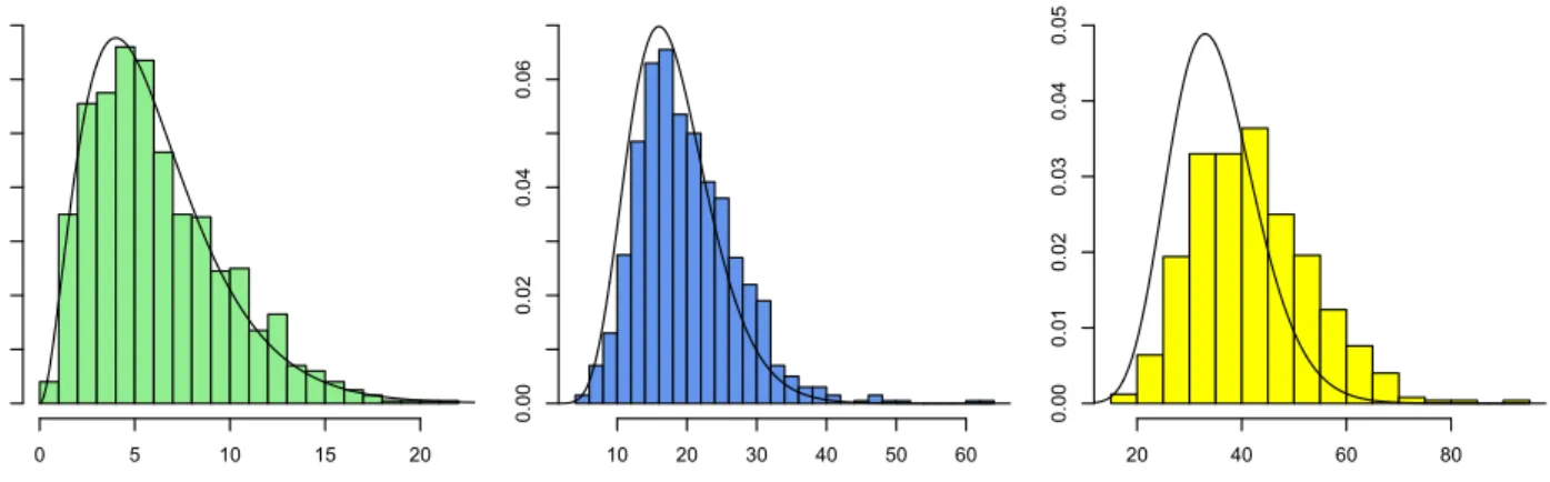
0 5 10 15 20 0.00 0.04 0.08 0.12 10 20 30 40 50 60 0.00 0.02 0.04 0.06 20 40 60 80 0.00 0.01 0.02 0.03 0.04 0.05
Figure 4: Histograms showing the increase in deviance associated with setting to zero any nested log-linear parameters with effects higher than orders (from left to right) seven, six and five respectively. This corresponds to removing 6, 18 and 35 parameters respectively; the relevantχ2density is plotted in each case.
1 2 3 4 5 6 7 8 9 10 11 12 13 14 (a) 1 2 3 4 5 6 7 8 (b)
Figure 5: (a) A hidden variable DAG used to generate samples for Section 7. (b) The latent projection of this generating DAG.
not really necessary in this case (though the higher order parameters may become necessary again if the state space of latent variables grows).
We generated distributions from the latent variable model associated with the DAG in Fig. 5 (a) as fol-lows: each of the six latent variables takes one of three states with equal probability, and each observed vari-able takes the value 0 with a probability generated as an independent uniform random variable on (0,1), conditional upon each possible value of its parents. For each of 1,000 distributions produced independently using this method, we generated a dataset of size 5,000. We then fitted the nested model generated by the graph in Fig. 5 (b) to each dataset by maximum like-lihood estimation, using a variation of an algorithm found in [5], and measured the increase in deviance associated with zeroing any nested ingenuous param-eters corresponding to effects above a certain order. If these parameters were truly zero, we would expect the increase to follow a χ2-distribution with an ap-propriate number of degrees of freedom; the first two histograms in Fig. 4 demonstrate that the distribution
of actual increases in deviance looks much like the rele-vantχ2-distribution if we remove interactions of order
6 and higher. The third histogram shows that this starts to break down slightly when 5-way interactions are also zeroed.
These results suggest that higher order parameters are often not useful for explaining finite datasets, and more parsimonious models can be obtained by remov-ing them; a similar simulation was performed for the Markov case in [6].
7.1 Distinguishing Graphs
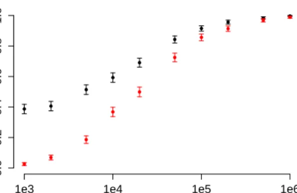
The use of score-based search methods for recovering nested Markov models had been investigated [15]. It was found that relatively large sample sizes were re-quired to reliably recover the correct graph, even in examples with only 4 or 5 binary nodes and after en-suring that the underlying distributions were approx-imately faithful to the true graph. One phenomenon identified was that incorrect but more parsimonious graphs, especially DAGs, tended to have lower BIC scores than the correct models, which include higher order parameters. Although BIC is guaranteed to be smaller on the correct model asymptotically, in finite samples it applies strong penalties for having addi-tional parameters with little explanatory power. Here we present a simulation to show how the new parameterization can help to overcome this difficulty. Using the method described in the previous subsec-tion, we generated 1,000 multivariate binary distribu-tions which were nested Markov with respect to the graph in Fig. 1 (b). For each distribution we gen-erated a dataset, and fitted the data to the correct model, which has 16 parameters, as well as the two DAGs given in Fig. 7 (a) and (b), which each have
1e3 1e4 1e5 1e6 0.0 0.2 0.4 0.6 0.8 1.0 Sample Size
Figure 6: From the experiment in Section 7.1: in red, the proportion of times graph in Fig. 1 (b) had lower BIC than the DAGs in Fig. 7, for varying sample sizes; in black, the proportion of times some restricted ver-sion of this model had a lower BIC than any restricted versions of either DAG.
11 parameters. This was repeated at various sample sizes.
The plot in Fig. 6 shows, in red, the proportion of times in which the BIC score for the correct model was lower than that for each of the DAGs, at various sample sizes. The correct graph only has the lowest BIC score of the three graphs on less than 3% of runs at sample size ofn= 1,000, increasing to around 50% forn= 20,000.
In addition to the full models, we fitted the datasets to versions of the models with higher order parameters removed; the graph in Fig. 1 (b) can be restricted by zeroing the 5-way parameter (leaving 15 free parame-ters), the 4-way and and above (13 params), or 3-way and above (10 params). Similarly we can restrict the DAGs to have no 3-way effects, giving each model 10 free parameters. Fig. 6 shows, in black, the proportion of times that one of these restricted versions of the true model had a lower BIC than any version of either DAG model. We see that the correct graph has the lowest score in 40% of runs at n = 1,000, rising to around 70% atn= 20,000. Note that these results should not be compared directly to those in [15], since the single ground truth law used in that paper was generated so as to ensure faithfulness to the correct graph, whereas we are randomly sampling multiple laws without both-ering to ensure any particular properties in these laws other than consistency with the underlying DAG. These results suggest that these submodels of the nested model may be advantageous in recovering the correct graphical structure using score-based methods.
1 2 3 4
5
(a) 1 2 3 4
5 (b)
Figure 7: (a) and (b) two DAGs with the same skeleton as the graph in Fig. 1 (b).
Note that determining which higher order parameters should be set to zero for a given data set and sample size remains non-trivial. Automatic selection might be possible with anL1-penalized approach [16, 4].
8
Discussion and Conclusions
We have introduced a new log-linear parameterization of nested Markov models over discrete state spaces. The log-linear parameters correspond to ‘interactions’ in kernels obtained after an iterative application of truncation and marginalization steps (informally ‘in-teractions in interventional densities’). By contrast the M¨obius parameters [15] correspond to context specific effects in kernels (informally ‘context specific causal effects’).
We have shown by means of a simulation study that in cases where data is generated from a marginal of a DAG with ‘weak confounders’, we can reduce the dimension of the model by ignoring higher order in-teraction parameters, while retaining the advantages of nested Markov models compared to modeling weak confounding directly in a DAG.
Though there is no efficient, closed form mapping from ingenuous parameters to either M¨obius parameters or standard probabilities, this is a smaller disadvantage than it may seem. This is because in cases where the ingenuous parameterization was used to select a particular submodel based on a dataset, we may still reparameterize and use M¨obius parameters, or even standard joint probabilities if desired. Moreover, this reparameterization step need only be performed once, compared to multiple calls to a fitting procedure which identified the particular graph corresponding to our submodel in the first place.
The ingenuous and the M¨obius parameterizations are thus complementary. The natural application of the ingenuous parameterization is in learning graph struc-ture from data in situations where many samples are not available, but we expect most confounding to be weak. The natural application of the M¨obius param-eterization is the support of probabilistic and causal inference in a particular graph [14, 15], in cases where an efficient mapping from parameters to joint proba-bilities is important.
References
[1] D. H. Ackley, G. E. Hinton, and T. J. Seinowski. A learning algorithm for boltzmann machines.Cognitive Science, 9(1):147–169, 1985.
[2] W. P. Bergsma and T. Rudas. Marginal models for categorical data. Annals of Statistics, 30(1):140–159, 2002.
[3] M. Drton and T. S. Richardson. Binary models for marginal independence. Journal of the Royal Statisti-cal Society (Series B), 70(2):287–309, 2008.
[4] R. J. Evans. Parametrizations of Discrete Graphical Models. PhD thesis, Department of Statistics, Univer-sity of Washington, 2011.
[5] R. J. Evans and A. Forcina. Two algorithms for fitting constrained marginal models. Computational Statis-tics & Data Analysis, 66:1–7, 2013.
[6] R. J. Evans and T. S. Richardson. Marginal log-linear parameters for graphical Markov models. Journal of the Royal Statistical Society (Series B) (to appear), 2013.
[7] D. Geiger, D. Heckerman, H. King, and C. Meek. Stratified exponential families: Graphical models and model selection. Annals of Statistics, 29(2):505–529, 2001.
[8] S. L. Lauritzen. Graphical Models. Oxford, U.K.: Clarendon, 1996.
[9] N. Meinshausen and P. B¨uhlmann. High-dimensional graphs and variable selection with the lasso. Annals of Statistics, 34(3):1436–1462, 2006.
[10] J. Pearl. Probabilistic Reasoning in Intelligent Sys-tems. Morgan and Kaufmann, San Mateo, 1988. [11] T. S. Richardson, J. M. Robins, and I. Shpitser.
Nested Markov properties for acyclic directed mixed graphs. In28th Conference on Uncertainty in Artifi-cial Intelligence (UAI-12). AUAI Press, 2012. [12] T. Rudas, W. P. Bergsma, and R. Nemeth.
Parame-terization and estimation of path models for categor-ical data. InProceedings in Computational Statistics, 17th Symposium, pages 383–394. Physica-Verlag HD, 2006.
[13] G. E. Schwarz. Estimating the dimension of a model.
Annals of Statistics, 6:461–464, 1978.
[14] I. Shpitser, T. S. Richardson, and J. M. Robins. An efficient algorithm for computing interventional dis-tributions in latent variable causal models. In 27th Conference on Uncertainty in Artificial Intelligence (UAI-11). AUAI Press, 2011.
[15] I. Shpitser, T. S. Richardson, J. M. Robins, and R. J. Evans. Parameter and structure learning in nested Markov models. In UAI Workshop on Causal Struc-ture Learning 2012, 2012.
[16] R. Tibshirani. Regression shrinkage and selection via the lasso.Journal of the Royal Statistical Society (Se-ries B), 58(1):267–288, 1996.
[17] T. S. Verma and Judea Pearl. Equivalence and synthe-sis of causal models. Technical Report R-150, Depart-ment of Computer Science, University of California, Los Angeles, 1990.