Arnu Pretorius
Dissertation presented for the degree of Doctor of Philosophy
in the Faculty of Science at Stellenbosch University
Computer Science Division,
Department of Mathematical Sciences,
University of Stellenbosch,
Private Bag X1, Matieland 7602, South Africa.
Promoters:
Dr R. S. Kroon Dr H. Kamper
Declaration
By submitting this dissertation electronically, I declare that the entirety of the work
con-tained therein is my own, original work, that I am the sole author thereof (save to the
extent explicitly otherwise stated), that reproduction and publication thereof by
Stellen-bosch University will not infringe any third party rights and that I have not previously
in its entirety or in part submitted it for obtaining any qualification.
This dissertation includes five original papers (two published and three under review).
The development and writing of the papers were the principal responsibility of myself
and, for each of the cases where this is not the case, a contribution statement is included
in the dissertation indicating the nature and extent of the contributions of co-authors.
Date:
December 2019
Copyright © 2019 Stellenbosch University
All rights reserved.
Abstract
On
Noise
Regularised
Neural
Networks:
Initialisation,
Learning
and
Inference
A.
Pretorius
Computer
Science
Division,
Department
of
Mathematical
Sciences,
University
of
Stellenbosch,
Private
Bag
X1,
Matieland
7602,
South
Africa.
Dissertation:
PhD
(Computer
Science)
December
2019
Innovation in regularisation techniques for deep neural networks has
been a key factor
in
the
rising
success
of
deep
learning.
However,
there
is
often
limited
guidance
from
theory
in
the
development
of
these
techniques
and
our
understanding
of
the
functioning
of various
successful
regularisation
techniques
remains
impoverished.
In
this
work,
we
seek
to
contribute
to
an
improved
understanding
of
regularisation
in
deep
learning.
We
specifically f ocus o n a
p articular a pproach t o r egularisation that
injects
noise
into
a
neural
network.
An
example
of
such
a
technique
which
is
often
used
is
dropout
(Srivastava
et
al.
, 2014).
Our
contributions
in
noise
regularisation
span
three
key areas
of
modeling:
(1)
learn-ing,
(2)
initialisation
and
(3)
inference.
We
first a nalyse t he l earning d ynamics o f a
simple
class
of
shallow
noise
regularised
neural
networks
called
denoising
autoencoders
(DAEs)
(Vincent
et
al.
,
2008),
to
gain
an
improved
understanding
of
how
noise
affects
the
learning
process.
In
this
first p art, w e o bserve a
d ependence o f l earning behaviour
on
initialisation,
which
leads
us
to
study
how
noise
interacts
with
the
initialisation
of
a
deep
neural
network
in
terms
of
signal
propagation
dynamics
during
the
forward
and
backward
pass.
Finally,
we
consider
how
noise
affects
inference
in
a
Bayesian
context.
We mainly
focus on fully-connected feedforward
neural
networks with rectifier linear unit
(ReLU)
activation
functions
throughout
this
study.
To
analyse
the
learning
dynamics
of
DAEs,
we
derive
closed
form
solutions
to
a
sys-tem
of
decoupled differential
equations
that
describe
the
change
in scalar
weights
during
the
course
of
training
as
they
approach
the
eigenvalues
of
the
input
covariance
matrix
(under
a
convenient change of basis).
In
terms
of
initialisation,
we
use mean
field theory
to
approximate
the
distribution of
the
pre-activations of
individual
neurons,
and
use
this
to
derive
recursive
equations
that
characterise
the
signal
propagation
behaviour
of
the
noise
regularised
network
during
the
first forward and backward pass of t raining. Using
these equations, we derive new initialisation schemes for noise regularised neural networks
that ensure stable signal propagation.
Since this analysis is only valid at initialisation, we
next
conduct
a
large-scale
controlled
experiment,
training
thousands
of
networks
under
tion on training speed and generalisation. To shed light on the influence of noise on
inference, we develop a connection between randomly initialised deep noise regularised
neural networks and Gaussian processes (GPs)—non-parametric models that perform
ex-act Bayesian inference—and establish new connections between a particular initialisation
of such a network and the behaviour of its corresponding GP. Our work ends with an
application of signal propagation theory to approximate Bayesian inference in deep
learn-ing where we develop a new technique that uses
self-stabilising priors
for training deep
Bayesian neural networks (BNNs).
Our core findings are as follows: noise regularisation helps a model to focus on the
more prominent statistical regularities in the training data distribution during learning
which should be useful for later generalisation. However, if the network is deep and not
properly initialised, noise can push network signal propagation dynamics into regimes of
poor stability. We correct this behaviour with proper “noise-aware” weight initialisation.
Despite this, noise also limits the depth to which networks are able to train successfully,
and networks that do not exceed this depth limit demonstrate a surprising insensitivity to
initialisation with regards to training speed and generalisation. In terms of inference, noisy
neural network GPs perform best when their kernel parameters correspond to the new
initialisation derived for noise regularised networks, and increasing the amount of injected
noise leads to more constrained (simple) models with larger uncertainty (away from the
training data). Lastly, we find our new technique that uses self-stabilising priors makes
training deep BNNs more robust and leads to improved performance when compared to
other state-of-the-art approaches.
Opsomming
Ruisgeregulariseerde
Neurale
Netwerke:
Inisialisering,
Leer
en
Inferensie
A.
Pretorius
Rekenaarwetenskap
Afdeling,
Departement
van
Wiskundige
Wetenskappe,
Universiteit
van
Stellenbosch,
Privaatsak
X1,
Matieland
7602,
Suid
Afrika.
Proefskrif:
PhD
(Rekenaarwetenskap)
Desember 2019
Innovasie in regulariseringstegnieke vir diep neurale netwerke is ’n belangrike aspek van die
toenemende sukses van diepleer.
Daar is egter beperkte teoretiese leiding in die
ontwikke-ling van hierdie tegnieke, en ons begrip van hoe verskeie suksesvolle regulariseringstegnieke
funksioneer
is
steeds
onvolledig.
Hierdie
proefskrif
poog
om
’n
bydra
te
maak
tot
’n
beter
begrip
van
regularisering
in
diepleer.
Ons
fokus
spesifiek o p b enaderings w at van r uis g ebruik m aak o m neurale
netwerke
te
regulariseer.
Een
voorbeeld
van
so
’n
tegniek
wat
gereeld
gebruik
word,
is
weglating
(“dropout”)
(Srivastava
et
al.
,
2014).
Ons
bydrae
tot
ruisregularisering
span
drie
sleutelareas
van
modellering:
(1)
leer,
(2)
inisialisering en (3) inferensie.
Ons ondersoek eers die leerdinamika van ’n eenvoudige klas
van
vlak
ruisgeregulariseerde
neurale
netwerke,
genaamd
ontruisende
outo-enkodeerders
(DAEs)
(Vincent
et
al.
,
2008),
om
’n
beter
begrip
te
kry
van
hoe
ruis
die
leerproses
beïnvloed.
In
die
eerste
deel,
neem
ons
waar
dat
leergedrag
afhanklik
is
van
inisialise-ring.
Dit
motiveer
’n
studie
waar
ons
die
wisselwerking
tussen
ruis
en
die
inisialisering
van
diep
neurale
netwerke
bestudeer
in
terme
van
die
dinamika
van
seinvloei
gedurende
die
aanvanklike
voorwaartse
en
terugwaartse
deurvloei.
Laastens
word
daar
gekyk
na
die
invloed
van
ruis
in
die
Bayes-konteks.
Hierdie
studie
fokus
hoofsaaklik
op
volledig-gekoppelde vorentoevoer
neurale
netwerke met die
gerektifiseerde lineêre eenheid (ReLU)
aktiveringsfunksie.
Om
die
leerdinamika
van
DAEs
te
ontleed,
lei
ons
geslotevorm
oplossings
af
vir
’n
stelsel ontkoppelde differensiaalvergelykings
wat
die verandering in skalaargewigte
tydens
die
afrigproses
beskryf,
soos
wat
hulle
na
die
eiewaardes
van
die
toevoerkovariansiema-triks
neig
(onder
’n
gerieflike b asisverandering). Wat i nisialisering b etref, g ebruik ons
gemiddelde-veldteorie
om
die
verdeling
van
die
voor-aktiverings
van
individuele
neurone
te
benader,
en
gebruik
ons
dan
hierdie
resultate
om
rekursiewe
vergelykings
af
te
lei
wat
die
seinvloei
gedrag
van
ruisgeregulariseerde
netwerke
tydens
die
eerste
voorwaartse
en
terugwaartse
deurvloei
beskryf.
Ons
gebruik
hierdie
vergelykings
om
nuwe
inisiali-seringskemas
vir
ruisgeregulariseerde
neurale
netwerke
wat
stabiele
seinvloei
verseker
te
skaalse gekontroleerde eksperiment uit deur duisende netwerke af te rig volgens ’n geskikte
eksperimentele ontwerp, om sodoende die effek van inisialisering op die afrigspoed en
ver-algemening van die afrigte netwerke te toets. Om lig te werp op die effek van ruis op
inferensie, ontwikkel ons ’n verband tussen ewekansigge geïnitialiseerde diep
ruisgeregu-lariseerde neurale netwerke en Gaussiese prosesse (GPs)—nie-parametriese modelle wat
presiese Bayesiaanse inferensie uitvoer—sowel as nuwe verbande tussen ’n spesifieke
inisi-alisering van die netwerk en die optrede van die ooreenstemmende GP. Die proefstuk word
afgesluit met ’n toepassing van seinvloeiteorie op Bayesiaanse inferensie in diep neurale
netwerke, waar ons ’n nuwe tegniek, wat gebruik maak van “
selfstabiliserende priors
”,
ontwikkel.
Ons kernbevindinge is as volg: ruisregularisering help ’n model om te fokus op die
meer prominente statistiese reëlmatighede in die verdeling van die afrigdata, wat vir
la-tere veralgemening nuttig behoort te wees. As die netwerk egter diep is en nie behoorlik
geïnisialiseer is nie, kan ruis veroorsaak dat die dinamika van die netwerk se seinvloei
onstabiel raak. Ons kan egter hierdie optrede teenwerk met behoorlike “ruisbewuste”
ge-wigsinisialisering. Nietemin, beperk ruis die diepte waartoe netwerke suksesvol afgerig
kan word, en netwerke wat nie hierdie dieptebeperking oorskry nie, toon ’n verbasende
onsensitiwiteit tot inisialisering met betrekking tot hul afrigspoed en veralgemening. Wat
inferensie betref, presteer ruisige neurale netwerk GPs die beste wanneer hul
kernparame-ters ooreenstem met die nuwe inisialisering wat afgelei is vir ruisgeregulariseerde netwerke,
en ’n toename in die hoeveelheid ruis wat bygevoeg word lei tot meer beperkte
(eenvou-dige) modelle met groter onsekerheid (weg van die afrigtingsdata). Laastens vind ons dat
ons nuwe tegniek, wat gebruik maak van “selfstabiliserende priors”, die afrigting van
Baye-siaanse neurale netwerke meer robuust maak en tot verbeterde prestasie lei in vergelyking
met ander moderne benaderings.
Acknowledgements
I would like to start by deeply thanking both my supervisors Dr Steve Kroon and Dr
Herman Kamper. Steve, thank you for being so meticulous in your approach, for always
making the time to see me when I need your guidance or advice, and for being a wonderful
advisor. Herman, thank you for all your advice, support, encouragement and all the
numerous small discussions that made a world of difference (even if it did not feel to you
that way) for my confidence as a researcher. I have truly learned a lot from both of you.
I am extremely thankful for all my lab mates at the MIH Media Lab at Stellenbosch
University. You know who you are! Thanks for all the great conversations, ideas, games,
advice, tea, milk and just for being good company during countless late nights and early
mornings. Especially, Armand du Plessis, I’m going to miss our early morning
philosoph-ical discussions over a cup of tea.
I would also like to express my deepest thanks and gratitude to all the students who
have worked with me on some of the research projects in this dissertation, either as
participants in initial coding sprints or as full research collaborators: Elan van Biljon,
Felix McGregor, Benji van Niekerk, Ryan Eloff, Steve James and Matthew Reynard. It
was truly a pleasure to work with all of you. Special thanks to Elan van Biljon. You are
a great friend and all-round wonderful person to work with.
I would like to thank Dr McElory Hoffmann and Dirko Coetsee from Praelexis for
letting me do some of my research in their workspace and for stimulating conversations
throughout this time. Also, a special thanks to Dr Bubacarr Bah for inviting me to
give talks on my research at the Southern African Mathematical Science Association
(SAMSA) Conference and at the African Institute for Mathematical Sciences (AIMS) in
South Africa.
I would also like to thank Dr Benjamin Rosman for inviting me to give a talk at the
RAIL lab at Wits University. The RAIL lab is home to truly some of the most impressive
researchers and students on the African continent. Your high and consistent achievements
have really inspired me to always try my best and reach for ambitious goals.
The
Deep Learning Indaba
(DLI), the largest annual meeting of the African machine
learning community, has shaped my trajectory as a young aspiring researcher enourmously.
I would therefore like to deeply thank the following people who are behind this great
initia-tive to strengthen machine learning in Africa: Shakir Mohamed, Ulrich Paquet, Avishkar
Bhoopchand, Stephan Gouws, Benji Rosman, Willie Brink, Vukosi Marivate, Nyalleng
Moorosi, Richard Klein, Muthoni Wanyoike, Kathleen Siminyu, Daniela Massiceti and
Herman Kamper. The impact the DLI has had over the years, not just on me, but on the
entire international community, is truly amazing. We as a community cannot thank you
enough.
I am especially indebted to Ulrich Paquet, who has been a wonderful mentor and a
friend. Thank you for your support and advice, letting me stay with you during my visit
to the UK and introducing me to the Computational and Biological Learning (CBL) lab
I would like to thank the following funding sources who have supported me at various
stages during my research: the Centre for Artifical Intelligence Research (CAIR) in South
Africa, the Harry Crossley foundation, Google, Nvidia, NeurIPS and ICML.
Second to last, a huge thank you to all my family and friends! Specifically my parents,
Otto Pretorius and Ina Pretorius, thank you for your tremendous encouragement and
support throughout my graduate years. And my brothers Ruan Pretorius and Daru
Pretorius, for always being there for me when I need you, even though you have no idea
what I’m actually doing half of the time.
Lastly, I would like to thank my wife, Jani Pretorius. From the bottom of my heart,
thank you for all your love, kindness, understanding and support. Without you none of
this would have been possible.
Contents
Declaration
i
Abstract
ii
Opsomming
iv
Acknowledgements
vi
Contents
viii
1 Introduction
1
1.1 Supervised machine learning . . . .
1
1.2 Deep learning . . . .
3
1.3 Regularisation . . . .
4
1.4 Thesis contributions . . . .
5
2 Learning dynamics of denoising autoencoders
8
2.1 Introduction . . . .
8
2.2 Background . . . .
9
2.3 Contribution statement . . . 10
2.4 Discussion . . . 24
3 Initialisation strategies for noise regularised neural networks
25
3.1 Introduction . . . 25
3.2 Background . . . 26
3.2.1 Mean field theory for neural networks . . . 27
3.3 Contribution statement . . . 28
3.4 Discussion . . . 49
4 At limited depth, can we initialise better?
50
4.1 Introduction . . . 50
4.2 Contribution statement . . . 51
4.3 Discussion . . . 67
5 Noise regularised neural networks as Gaussian processes
68
5.1 Introduction . . . 68
5.2 Background . . . 69
5.3 Contribution statement . . . 70
5.4 Discussion . . . 83
6.1 Introduction . . . 84
6.2 Background . . . 85
6.3 Contribution statement . . . 86
6.4 Discussion . . . 95
7 Conclusions
96
7.1 Summary . . . 96
7.2 Future work . . . 97
List of references
99
Chapter 1
Introduction
Regularisation plays a central role in deep learning. However, several state-of-the-art
innovations in regularisation are still only heuristically motivated, or have largely come
about through experimentation. As a result, we still lack a solid understanding of how
and why different regularisation strategies work, and in what ways these strategies affect
the different stages of modeling. Furthermore, a better understanding of regularisation
for deep learning might enable a more principled approach to neural network design and
regularisation.
The aim of this thesis
is to contribute towards an improved understanding of
regularisation for deep learning. We focus on a particular regularisation strategy that
injects noise into a neural network during training. This strategy has been shown to be
especially effective for a wide range of different deep learning models and applications
(Sietsma and Dow,
1991;
Vincent
et al.
,
2008;
Srivastava
et al.
,
2014).
The outline of this thesis
is as follows: the remainder of this introductory chapter
will provide general background relevant for contextualising the contributions in this
thesis. Chapters 2 to 6 form the main content of the thesis. Each chapter is based on
a paper and consists of an introduction, a contribution statement, the paper itself and a
discussion. We also provide background material separately in each chapter as required.
Finally, we conclude in Chapter 7 with a summary of the thesis and suggested future
work.
1.1
Supervised machine learning
Statistical machine learning aims to create intelligent computer systems capable of
mak-ing appropriate decisions in a variety of complex situations. Typically, these computer
systems acquire their decision-making ability through
machine learning algorithms
. By
combining data collected from the real world with an assumed statistical model
describ-ing the relationships between examples, machine learndescrib-ing algorithms learn how to make
decisions through error correction by optimising a pre-specified
objective function
.
More specifically, it is possible to implement a wide variety of well-known supervised
machine learning algorithms using the following generic template: given a data set of
independent and identically distributed (i.i.d.) input-output pairs
D
=
{
(
x
i, y
i)
, i
=
1
, ..., N
}, we assume a probability distribution for
y
given
x
of the form
y
|
x
∼
p
(
α
)
, where
α
represents a set of parameters describing the distribution (e.g.
µ
and
σ
2, the mean and
variance describing a Gaussian distribution). To model the expected relationship
E
[
y
|
x
]
,
we use a parameterised function of the input
f
(
x
, θ
)
, where the adjustable parameters
Finally, we estimate suitable parameters
θ
by maximising the likelihood of the parameters
given the observed data, or equivalently, minimising the negative log-likelihood
L
(
D
, θ
) =
N
X
i=1
−
log
p
(
y
i|
x
i, θ
)
.
(1.1.1)
Many (but not all) supervised machine learning algorithms can be considered as special
cases of the above general construction. A powerful alternative modeling paradigm is
Bayesian machine learning, which we discuss in Chapters 5 and 6.
These machine learning algorithms aim to uncover statistical regularities in the data
that describe the underlying data generating mechanism, and encode its typical behaviour
in the model parameters during learning. This task is far from simple, and tractable
approaches often rely on strong prior beliefs that are assumed to resonate with natural
phenomena of interest.
For example, using the above generic template, if we assume a Gaussian conditional
distribution
y
|
x
∼ N
(
f
(
x
, θ
)
, σ
2)
, with
f
(
x
, θ
=
{
w
, b
}
) =
w
·
x
+
b
, we obtain the
algorithm for
linear regression
, with squared-error loss:
L
(
D
, θ
)
∝
P
Ni=1(
f
(
x
i, θ
)
−
y
i)
2.
Here,
w
and
b
are the adjustable parameters of the model, referred to as the weights and
the bias respectively. Similarly, if we assume
y
|
x
is Bernoulli distributed with parameter
f
(
x
, θ
) =
ξ
(
w
·
x
+
b
)
, where
ξ
is the logistic function, we obtain
logistic regression
. These
two algorithms in particular have proved to be very useful for a wide range of different
regression and classification tasks. However, at their core is the assumption of
local
smoothness
in the input space, i.e.
f
(
x
)
≈
f
(
x
+
)
, for some small perturbation vector
. If observed data densely populate the input space, local smoothness is a reasonable
assumption and learned relationships generally extrapolate well to other unobserved areas
of the space.
Unfortunately, many real-world phenomena are embedded in extremely high
dimen-sional spaces. This leads to poor sample efficiency, requiring exponentially more data
per dimension to maintain the same level of local density. For a fixed number of data
points and a growing number of input dimensions, what is considered local in terms of
the nearest neighbours to a point in the input space, can no longer be considered local
in terms of the volume of space required to encapsulate all these neighbouring points.
This is often referred to as the
curse of dimensionality
(Bellman,
1961), and many
tradi-tional machine learning algorithms suffer from it (including popular kernel and tree-based
methods) (Hastie
et al.
,
2009).
One approach to overcoming the curse of dimensionality is to disentangle the
fac-tors of variation in the input representation by transforming the facfac-tors into
distributed
representations
(Goodfellow
et al.
,
2016). To see why this can be effective, consider a
data generator that produces images of cats and dogs, that can either be black or white
in colour. Instead of having representations encoding each different class e.g.
black-Cat, whiteblack-Cat, blackDog, whiteDog
, sometimes referred to as
localist
representations,
dis-tributed representations disentangle the factors of variation into colour
{
black, white
}
and
animal
{
cat, dog
}
and can construct all possible combinations as the Cartesian product
of the two sets. More generally, given an input vector
x
of size
d
, with binary encoding at
each index, a unique localist representation for each configuration would require collecting
O
(2
d)
data points to have knowledge of all possible configurations. In contrast, using a
distributed representation would only require
O
(
d
)
data points to obtain the same level
factors of variation in extremely complex observed phenomena can be very difficult. Hand
engineered preprocessing techniques, or
feature engineering
, is one approach, but usually
requires expert domain knowledge which limits its applicability in domains that are still
poorly understood, e.g. language development in infants (Räsänen,
2012;
Räsänen and
Rasilo,
2015). An alternative approach is to instead
learn
distributed representations.
1.2
Deep learning
Deep learning
attempts to learn distributed representations as part of a more general
purpose approach to statistical machine learning. The primary assumptions underlying
deep learning are: (1) most observed data stem from data generating mechanisms that are
compositional
in nature; and (2) that this hierarchical composition consists of independent
factors of variations at different levels of abstraction (i.e. representations are distributed
across both basic low-level concepts and higher-level complex or more abstract concepts)
(Goodfellow
et al.
,
2016). Deep learning still follows the same design pattern as the generic
template presented earlier for constructing different machine learning algorithms. It also
relies on the local smoothness assumption. But what is important, is that for many tasks
of interest the additional assumptions of (1) and (2) above tend to hold, and deep learning
is able to
overcome the curse of dimensionality by combining distributed representations
with composition
.
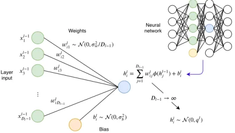
For example, a deep learning approach to modeling a continuous output variable
y
,
might follow the same recipe as linear regression, except that now
f
(
x
, θ
) =
w
out·
x
L+
b
out,
(1.2.1)
where the original input
x
is first transformed into
x
Lusing a multi-layered
deep neural
network
:
x
l=
φ
(
h
l)
,
space
h
l=
W
lx
l−1+
b
l,
space
for
l
= 1
, ..., L
(1.2.2)
with input
x
0=
x
. Here
φ
is an element-wise
activation function
, the
W
lare the weight
matrices, and
b
lare the bias vectors. We refer to
h
las the vector of hidden unit
pre-activations
and to
x
las the vector of hidden unit
activations
associated with a specific
layer
l
. The above network is an example of an
L
-hidden-layer
fully-connected feedforward
neural network with a linear output layer. The terms “fully-connected” and “feedforward”
refer to the
architecture
of the network. Different architectures attempt to create different
structural priors that are well suited for a particular task. Other popular architectures
include,
convolutional
architectures (LeCun,
1989) for spatial data and
recurrent
archi-tectures (Rumelhart
et al.
,
1988;
Hochreiter and Schmidhuber,
1997) for temporal data.
The network
f
(
x
, θ
)
is parameterised by
θ
=
{
w
out, b
out,
b
1, ...,
b
L, W
1, ..., W
L}, where
at each layer of the network the inputs are transformed by the weights
W
land bias vectors
b
land then passed through an activation functions
φ
. By learning through multiple
stacked layers in this way, the network is able to encode into the parameters suitable
transformations required to create hierarchically composed distributed representations of
the inputs. These representations then make downstream regression or classification tasks
more tractable when dealing with complex high-dimensional data.
Deep learning has made remarkable progress on long-standing and fundamental
chal-lenges in machine learning and artificial intelligence. It has been hugely successful for
Szegedy
et al.
,
2013;
Erhan
et al.
,
2014) and speech (Hinton
et al.
,
2012;
Graves and
Jaitly,
2014), generate comprehensible text (Sutskever
et al.
,
2011;
Graves,
2013), and
translate sentences (Cho
et al.
,
2014;
Sutskever
et al.
,
2014).
Although the idea of representation learning was the driving force behind the
devel-opment of deep learning, these algorithms still rely heavily on
regularisation
and clever
optimisation
, to be able to perform well. One way to think of deep learning is in terms of
search, where algorithms run the following procedure: (1) define a
hypothesis space
con-taining different possible hypotheses explaining the underlying data generating mechanism
and (2) search this space to find the hypothesis (a mapping from learned representations
to output) that best describes the general trends in the observed data. By respectively
playing key roles in steps (1) and (2) above, regularisation and optimisation form the
pillars of deep learning. In this thesis, we focus on regularisation.
1.3
Regularisation
Machine learning differs from pure optimisation in the sense that the task is to learn
from a finite collection of observed data (i.e. to optimise over some training set), but
then
generalise
to the underlying data generator of (possibly infinitely many) previously
unseen test observations. We assume that this is possible as long as the observed training
data and the test data come from the same distribution. If the samples that comprise
the training and test sets are i.i.d., the expected performance of a model for a given
set of parameters will be equal on both sets. However, during optimisation the model
parameters are specifically modified using information from the training set. If the model
starts to incorporate idiosyncrasies specific to the training set, it will not generalise well
to the true underlying distribution. This generally happens when the
complexity
of the
model is inappropriate for the task at hand.
The complexity of a model refers to the variety of functions it is able to express.
These functions can range from being too simple to fit the data (underfitting), to
be-ing unnecessarily complex (overfittbe-ing). For a fixed trainbe-ing set, an appropriate level of
complexity typically lies somewhere between these two extremes, as illustrated in Figure
1.1. A key result from
statistical learning theory
is that there exists an upper bound on
the difference between training and generalisation performance. This bound grows with
model complexity, but shrinks with dataset size (Vapnik,
1995).
Solutions in the hypothesis space will be associated with different levels of complexity.
When searching the hypothesis space, pure optimisation on the training set will favour
models of greater complexity, since these will correspond to the functions most capable
of minimising the training loss. Unfortunately this does not guarantee that the test loss
will also be low. On the contrary, the most common outcome in this situation is that the
model overfits and performs poorly on new test data. Therefore, pure optimisation is not
sufficient for developing useful machine learning algorithms. What we require in addition
to optimisation is effective regularisation.
Regularisation can broadly be defined as follows:
Definition 1: Regularisation
refers to any strategy that modifies or encodes
preferences into the hypothesis space being searched during optimisation, with
Loss Model Complexity Test Train Optimal Overfitting
Figure 1.1:
Model complexity, underfitting and overfitting
: The plot shows typical training and
test loss curves as a function of model complexity. Green circles represent training points and
orange squares represent test points, with fitted regression functions shown in blue.
Simply put, regularisation aims to ensure that optimisation on the training set is more
likely to translate into good performance on the test set. This does not mean that
reg-ularisation improves optimisation. In fact, the opposite is often the case, with added
regularisation leading to more difficult optimisation problems and reduced performance
on the training set. Instead, regularisation only serves as a way to build preferences
into the hypothesis space that guide the search procedure. This guidance is provided
irrespective of the difficulty in optimisation associated with each preference.
Regularisation can either be implicit, for example designing algorithms based on the
assumptions of smoothness and hierarchical composition. Alternatively, it can be more
explicit, such as directly limiting the hypothesis space or constraining the optimisation
procedure.
In this thesis, we focus on an explicit form of regularisation that injects noise into a
neu-ral network during training. Specifically, for an input
x
lat an arbitrary layer
l
= 0
,
1
, ..., L
,
in a deep neural network, we consider general noise injection of the form
x
˜
l=
x
ll
.
Here,
denotes element-wise addition or multiplication and
is a noise vector sampled
from a pre-specified noise distribution. We refer to this specific form of regularisation
simply as
noise regularisation
. We consider in our investigations both additive and
mul-tiplicative noise sampled from different noise distributions and injected at different layers
of the network.
1.4
Thesis contributions
Our contributions focus on understanding the effect of noise regularisation on different
stages of the modeling process, namely at initialisation (the setting of the starting
parame-ter values), during learning (optimisation) and when performing inference (prediction and
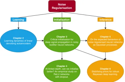
uncertainty estimation). See Figure 1.2 for a visual overview.
In each chapter
we make the following contributions:
•
Chapter 2
investigates the learning dynamics of linear autoencoder neural networks
with input noise injection. We derive new closed-form solutions to the learning
dynamics of these models in expectation over the sampled noise. We find that noise
helps the model to avoid learning low variance directions in the input space, while
leaving higher variance directions largely unaffected. Our findings also highlight
Chapter 2 Learning dynamics of linear
denoising autoencoders
Chapter 3 Critical initialisation for deep signal propagation in noisy
rectifier neural networks.
Chapter 4 At limted depth, can we initialise
better? An empirical study on ReLU networks
with dropout.
Chapter 5 On the expected behaviour of noise regularised neural networks
as Gaussian processes.
Chapter 6 Stabilising priors for robust
Bayesian deep learning.
Learning Initialisation Inference
Figure 1.2:
Contributions: outline, flow and dependencies
. Our contributions fall into three
broad categories: learning (blue), initialisation (green) and inference (orange). Black arrows show
dependencies between papers. For example, Chapter 4 builds on work presented in Chapter 3,
and Chapter 6 was influenced by the ideas in Chapters 3 and 5.
the effects of noise from different initialisations, as well as provide connections with
other well-known regularisation techniques such as weight decay and early stopping.
Specifically, noise regularisation is shown to have a similar regularisation effect as
weight decay, but with faster training dynamics.
Paper: Pretorius, A., Kroon, S., & Kamper, H. Learning dynamics of linear denoising
autoencoders. International Conference on Machine Learning (ICML, 2018).
•
Chapter 3
moves to the nonlinear case and focuses specifically on initialisation for
noise regularised neural networks. We investigate how noise interacts with
initiali-sation during the forward pass in deep fully-connected feedforward neural networks
that use Rectified Linear Unit (ReLU) activation functions. We derive a new
crit-ical initialisation for noise regularised neural networks that is optimal in terms of
specific criteria for stable forward signal propagation. Our initialisation also helps
to shed light on previously unexplained phenomena, for example why a dropout rate
of
0
.
5
often works well in practice when combined with a well-known initialisation
strategy. Finally, we show how noise regularisation limits the maximum depth to
which a ReLU neural network can be trained.
Paper: Pretorius, A., van Biljon, E., Kroon, S. & Kamper, H. Critical initialisation for
deep signal propagation in noisy rectifier neural networks. Advances in Neural Information
Processing Systems (NeurIPS, 2018).
•
Chapter 4
directly builds on the work in Chapter 3 and investigates the following
question: if critical initialisation is only a requirement for
deep
signal propagation,
and noise
limits training depth
, are there perhaps alternative (non-critical)
initiali-sations that perform better for noisy networks within this depth limit? We perform
a large-scale controlled experiment by training over
12
,
000
networks to compare
critical versus non-critical initialisations. A statistical analysis of our results shows
that for a wide range of initialisations around criticality, there is no statistically
significant difference in training speed or generalisation when compared to the
crit-ical initialisation. Our analysis seems to indicate that neural networks of shallow to
moderate depth are largely insensitive to initialisation.
S., Rosman, B., Kamper, H., & Kroon, S. At limted depth, can we initialise better? An
empirical study on ReLU networks with dropout. Preprint (arXiv, 2019).
•
Chapter 5
connects noise regularised deep neural networks with Gaussian
pro-cesses (GPs). Prior work has shown that a deep neural network at initialisation is
equivalent in the large width limit to a GP. The resulting GP’s kernel parameters
depend on the network depth and the scale of the weights and biases. We extend
these results to include noise regularisation. We find that the best performing GPs
are those that have their kernel parameters set to correspond to the values
spec-ified by the initialisation derived in Chapter 3. Furthermore, we show how noise
regularisation in a neural network affects the covariance of the corresponding noisy
GP. As more noise is injected into the network, the covariance tends to become
diagonal implying complete independence between training points. This leads to a
stronger prior for simple functions and larger uncertainty in the posterior predictive
distribution when performing exact Bayesian inference.
Paper: Pretorius, A., Kamper, H., & Kroon, S. On the expected behaviour of noise
regularised neural networks as Gaussian processes. Preprint (arXiv, 2019).
•
Chapter 6
considers approximate Bayesian inference in deep Bayesian neural
net-works (BNNs). Inspired by the analysis techniques in Chapters 3 and 5, we develop
self-stabilising priors
, an adaptive Monte Carlo variational inference method for
BNNs. This approach is able to successfully train much deeper BNNs in more noisy
settings (with large uncertainty in the weights) than other state-of-the-art methods.
Paper: McGregor, F., Pretorius, A., du Preez, J., & Kroon, S. Stabilising priors for robust
Bayesian deep learning. Advances in Neural Information Processing Systems workshop on
Bayesian Deep Learning (NeurIPS BDL workshop, 2019).
Finally, in
Chapter 7
we provide a summary of the work presented in the thesis along
with concluding remarks and suggestions for future work.
Chapter 2
Learning dynamics of denoising
autoencoders
Paper
Pretorius, A., Kroon, S., & Kamper, H. Learning dynamics of linear denoising autoencoders. International Conference on Machine Learning (ICML, 2018).
Available at: http://proceedings.mlr.press/v80/pretorius18a/pretorius18a.pdf
Code
Pretorius, A. (2018). Code for: Learning dynamics of linear denoising autoencoders.
Available at: https://github.com/arnupretorius/lindaedynamics_icml2018.
Noise Regularisation
Chapter 2
Learning dynamics of linear denoising autoencoders
Chapter 3
Critical initialisation for deep signal propagation in noisy
rectifier neural networks.
Chapter 4
At limted depth, can we initialise better? An empirical study on
ReLU networks with dropout.
Chapter 5
On the expected behaviour of noise regularised neural networks
as Gaussian processes.
Chapter 6
Stabilising priors for robust Bayesian deep learning.
Learning Initialisation Inference
2.1
Introduction
As mentioned in Chapter 1, the success of deep learning is built upon a modeling
ap-proach that seeks to
learn
, instead of hand engineer, useful features for a particular task.
Autoencoder (AE) neural networks are especially useful in this regard. AEs are frequently
used as
feature extractors
. A good feature extractor network learns useful latent feature
representations which are “extracted” from the internal layers of the network for use in
subsequent tasks.
During feature extraction, noise regularisation forces an AE network to focus on the
more generalisable statistical aspects of the input distribution. By ignoring less relevant
information (hopefully specific to the training set) a type of noise regularised AE called
a
denoising autoencoder
(DAE), which we consider in this chapter, generally learns more
However, even though DAEs are empirically very useful, our theoretical understanding of
how noise affects the learning of DAEs remains limited.
In this chapter, we investigate the dynamics of learning in DAEs to uncover how the
directions of variation in the input distribution are learned over the course of training.
Our approach largely follows that of
Saxe
et al.
(2014). Specifically, we focus on the
learning dynamics of
linear
DAEs in expectation over the noise distribution. Although
the models we study are linear, their
learning dynamics are nonlinear
and closely
resem-ble the learning dynamics empirically observed in nonlinear networks. We make use of a
convenient change of basis that aligns the weights with the directions of variation in the
input covariance. This allows the dynamics of learning to be described in terms of
indi-vidual scalar dynamics for each eigenvalue associated with a specific direction. We derive
exact solutions to differential equations describing the change in the map
approximat-ing each eigenvalue under the assumption of a small enough learnapproximat-ing rate for continuous
gradient descent dynamics. We find that the noise in DAEs helps the network to focus
on learning only the larger variance directions during training, while ignoring smaller
variance directions. We compare these dynamics with those for weight decay, a popular
form of regularisation that adds a weight norm penalty to the loss function (Krogh and
Hertz,
1992). Our analysis shows that the noise regularisation of DAEs has a similar
regularisation effect to weight decay, but with faster training dynamics. Lastly, we verify
that our theoretical predictions approximate learning dynamics on real-world data and
qualitatively match observed dynamics in nonlinear DAEs.
2.2
Background
Autoencoding neural networks (LeCun,
1987;
Bourlard and Kamp,
1988;
Hinton and
Zemel,
1994) attempt to learn an input data representation by modeling the inputs as the
expected outputs. Although autoencoding is a form of
unsupervised learning
(learning
without output labels), autoencoders generally follow the same generic template for
su-pervised machine learning algorithms as outlined in Chapter 1. Specifically, we assume a
distribution for the inputs conditioned on the inputs themselves and model the expected
value of this distribution using a parameterised function. To find the optimal parameters,
we minimise the negative log-likelihood.
The motivation behind autoencoder networks is as follows: if a layered network is able
to accurately predict its own input, it is likely that the representations in its intermediate
layers capture important characteristics of the input distribution. If this is the case, we
can extract these representations from the network and use them in various downstream
tasks. For this to be possible, the network model must be complex enough to capture
important variations in the input, but at same time, not be so complex that it can simply
represent the identity mapping. Therefore, for autoencoders to be useful, it is crucial that
they incorporate some form of regularisation.
An effective way to regularise autoencoders is to inject noise into their inputs (Vincent
et al.
,
2008). This type of regularised autoencoder is known as a
denoising autoencoder
(DAE). For example, we can consider a real-valued input
x
injected with additive isotropic
Gaussian noise, producing a corrupted version
x
˜
=
x
+
, where
∼ N
(
0
, s
2I
)
. By
f
(˜
x
, θ
) =
W
outx
L+
b
out,
where
x
l=
φ
(
h
l)
,
space
h
l=
W
lx
l−1+
b
l,
space
for
l
= 1
, ..., L
(2.2.1)
with
x
0= ˜
x
. When
L
= 1
, the internal representations of the input data get extracted
from a single intermediate hidden layer, i.e.
h
1.
An implicit assumption often useful when designing machine learning algorithms is
that almost all of the structure observed in the natural world resides on some
lower-dimensional manifold. As an example, consider image data. The number of pixel
config-urations that produce meaningful images of real-world objects is far less than the total
number of possible image configurations. Similar observations apply to many other
differ-ent data types, e.g. speech or text data (Silberer and Lapata,
2012;
Kamper
et al.
,
2015).
This means that we can expect the real-world input distributions we actually observe to
often be of a far smaller intrinsic dimension.
DAEs have been interpreted as a technique that pushes data off of its intrinsic
man-ifold using noise injection, only to learn how to map the data back onto this manman-ifold
(Vincent
et al.
,
2008). Reconstructing the original inputs in this way forces DAEs to
learn a type of (local) coordinate system. The axes of this coordinate system then span
the directions of variation in the input space that are useful for getting back onto the
manifold. Importantly, the directions orthogonal to this span, which are less useful for
reconstruction, get ignored in the learned representations.
2.3
Contribution statement
The idea for this work was inspired by discussions with Andrew Saxe at the 2016
PRASA-Robmech conference in Stellenbosch, South Africa. I derived the theoretical results,
per-formed the experiments and wrote the paper. Dr Steve Kroon provided technical feedback.
Dr Herman Kamper provided general feedback and useful editorial suggestions.
Learning Dynamics of Linear Denoising Autoencoders
Arnu Pretorius1 2 Steve Kroon1 2 Herman Kamper3Abstract
Denoising autoencoders (DAEs) have proven use-ful for unsupervised representation learning, but a thorough theoretical understanding is still lack-ing of how the input noise influences learnlack-ing. Here we develop theory for how noise influences learning in DAEs. By focusing on linear DAEs, we are able to derive analytic expressions that exactly describe their learning dynamics. We ver-ify our theoretical predictions with simulations as well as experiments on MNIST and CIFAR-10. The theory illustrates how, when tuned correctly, noise allows DAEs to ignore low variance direc-tions in the inputs while learning to reconstruct them. Furthermore, in a comparison of the learn-ing dynamics of DAEs to standard regularised autoencoders, we show that noise has a similar regularisation effect to weight decay, but with faster training dynamics. We also show that our theoretical predictions approximate learning dy-namics on real-world data and qualitatively match observed dynamics in nonlinear DAEs.*
1. Introduction
The goal of unsupervised learning is to uncover hidden struc-ture in unlabelled data, often in the form of latent feastruc-ture representations. One popular type of model, an autoencoder, does this by trying to reconstruct its input (Bengio et al., 2007). Autoencoders have been used in various forms to ad-dress problems in machine translation (Chandar et al.,2014; Tu et al.,2017), speech processing (Elman & Zipser,1987; Zeiler et al.,2013), and computer vision (Rifai et al.,2011; 1Computer Science Division, Stellenbosch University, South
Africa 2CSIR/SU Centre for Artificial Intelligence Research, 3Department of Electrical and Electronic Engineering,
Stellen-bosch University, South Africa. Correspondence to: Steve Kroon
Proceedings of the35thInternational Conference on Machine
Learning, Stockholm, Sweden, PMLR 80, 2018. Copyright 2018
by the author(s).
*Code to reproduce all the results in this paper is available at: https://github.com/arnupretorius/lindaedynamics icml2018
Larsson,2017), to name just a few areas. Denoising
au-toencoders (DAEs) are an extension of auau-toencoders which learn latent features by reconstructing data fromcorrupted versions of the inputs (Vincent et al.,2008). Although this corruption step typically leads to improved performance over standard autoencoders, a theoretical understanding of its effects remains incomplete. In this paper, we provide new insights into the inner workings of DAEs by analysing the learning dynamics of linear DAEs.
We specifically build on the work ofSaxe et al.(2013a;b), who studied the learning dynamics of deep linear networks in a supervised regression setting. By analysing the gradient descent weight update steps as time-dependent differential equations (in the limit as the learning rate approaches a small value),Saxe et al.(2013a) were able to derive exact solutions for the learning trajectory of these networks as a function of training time. Here we extend their approach to linear DAEs. To do this, we use the expected recon-struction loss over the noise distribution as an objective (requiring a different decomposition of the input covariance) as a tractable way to incorporate noise into our analytic solutions. This approach yields exact equations which can predict the learning trajectory of a linear DAE.
Our work here shares the motivation of many recent stud-ies (Advani & Saxe,2017;Pennington & Worah,2017;
Pennington & Bahri,2017;Nguyen & Hein,2017;Dinh
et al.,2017;Louart et al.,2017;Swirszcz et al.,2017;Lin et al.,2017;Neyshabur et al.,2017;Soudry & Hoffer,2017;
Pennington et al.,2017) working towards a better theoretical
understanding of neural networks and their behaviour. Al-though we focus here on a theory forlinearnetworks, such networks have learning dynamics that are in factnonlinear. Furthermore, analyses of linear networks have also proven useful in understanding the behaviour of nonlinear neural networks (Saxe et al.,2013a;Advani & Saxe,2017). First we introduce linear DAEs (§2). We then derive ana-lytic expressions for their nonlinear learning dynamics (§3), and verify our solutions in simulations (§4) which show how noise can influence the shape of the loss surface and change the rate of convergence for gradient descent optimi-sation. We also find that an appropriate amount of noise can help DAEs ignore low variance directions in the input while learning the reconstruction mapping. In the remainder of
the paper, we compare DAEs to standard regularised autoen-coders and show that our theoretical predictions match both simulations (§5) and experimental results on MNIST and CIFAR-10 (§6). We specifically find that while the noise in a DAE has an equivalent effect to standard weight decay, the DAE exhibits faster learning dynamics. We also show that our observations hold qualitatively for nonlinear DAEs.
2. Linear Denoising Autoencoders
We first give the background of linear DAEs. Given training data consisting of pairs{(˜xi,xi), i = 1, ..., N}, wherex˜
represents a corrupted version of the training datax∈RD,
the reconstruction loss for a single hidden layer DAE with activation functionφis given by
L= 1 2N N X i=1 ||xi−W2φ(W1˜xi)||2.
Here,W1 ∈RH×DandW2 ∈RD×H are the weights of the network with hidden dimensionalityH. The learned feature representations correspond to the latent variable
z=φ(W1x˜).
To corrupt an inputx, we sample a noise vector, where each component is drawn i.i.d. from a pre-specified noise distribution with mean zero and variances2. We define the corrupted version of the input asx˜ =x+. This ensures
that the expectation over the noise remains unbiased, i.e.
E(˜x) =x.
Restricting our scope to linear neural networks, withφ(a) =
a, the loss in expectation over the noise distribution is
E[L] = 1 2N N X i=1 ||xi−W2W1xi||2 whitece+s 2 2tr(W2W1W T 1W2T), (1)
See the supplementary material for the full derivation.
3. Learning Dynamics of Linear DAEs
Here we derive the learning dynamics of linear DAEs, be-ginning with a brief outline to build some intuition. The weight update equations for a linear DAE can be formu-lated as time-dependent differential equations in the limit as the gradient descent learning rate becomes small (Saxe et al.,
2013a). The task of an ordinary (undercomplete) linear
au-toencoder is to learn the identity mapping that reconstructs the original input data. The matrix corresponding to this learned map will essentially be an approximation of the full identity matrix that is of rank equal to the input dimension. It turns out that tracking the temporal updates of this map-ping represents a difficult problem that involves dealing with
coupled differential equations, since both the on-diagonal and off-diagonal elements of the weight matrices need to be considered in the approximation dynamics at each time step.
To circumvent this issue and make the analysis tractable, we follow the methodology introduced inSaxe et al.(2013a), which is to: (1)decompose the input covariance matrix using an eigenvalue decomposition;(2)rotate the weight matrices to align with these computed directions of vari-ation; and(3)use an orthogonal initialisation strategy to diagonalise the composite weight matrixW =W2W1. The important difference in our setting, is that additional con-straints are brought about through the injection of noise. The remainder of this section outlines this derivation for the exact solutions to the learning dynamics of linear DAEs.
3.1. Gradient descent update
Consider a continuous time limit approach to studying the learning dynamics of linear DAEs. This is achieved by choosing a sufficiently small learning rateαfor optimising
the loss in (1) using gradient descent. The update forW1 in a single gradient descent step then takes the form of a time-dependent differential equation
τ d dtW1= N X i=1 WT 2 xixTi −W2W1xixTi whitesp−εW2TW2W1 =W2T(Σxx−W2W1Σxx)−εW2TW2W1.
Heretis the time measured in epochs,τ = Nα, ε=N s2and Σxx=PNi=1xixTi, represents the input covariance matrix.
Let the eigenvalue decomposition of the input covariance be Σxx=VΛVT, whereV is an orthogonal matrix and denote
the eigenvaluesλj = [Λ]jj, withλ1 ≥ λ2 ≥ · · · ≥ λD.
The update can then be rewritten as
τ d dtW1=W T 2V Λ−VTW2W1VΛ VT morewhitespace−εWT 2W2W1.
The weight matrices can be rotated to align with the direc-tions of variation in the input by performing the rotadirec-tions
W1=W1V andW2=VTW2. Following a similar deriva-tion forW2, the weight updates become
τ d dtW1=W T 2 Λ−W2W1Λ−εW T 2W2W1 τ d dtW2= Λ−W2W1Λ WT1 −εW2W1W T 1.
3.2. Orthogonal initialisation and scalar dynamics
To decouple the dynamics, we can setW2=V D2RT and
andD2andD1are diagonal matrices. This results in the product of the realigned weight matrices
W2W1=VTV D2RTRD1VTV =D2D1 to become diagonal. The updates now reduce to the follow-ing scalar dynamics that apply independently to each pair of diagonal elementsw1jandw2jofD1andD2respectively:
τ d dtw1j =w2jλj(1−w2jw1j)−εw 2 2jw1j (2) τ d dtw2j =w1jλj(1−w2jw1j)−εw2jw 2 1j. (3)
Note that the same dynamics stem from gradient descent on the loss given by
`= D X j=1 λj 2τ(1−w2jw1j) 2+ D X j=1 ε 2τ(w2jw1j) 2. (4)
By examining (4), it is evident that the degree to which the first term will be reduced will depend on the magnitude of the associated eigenvalueλj. However, for directions in
the input covarianceΣxxwith relatively little variation the
decrease in the loss from learning the identity map will be negligible and is likely to result in overfitting (since little to no signal is being captured by these eigenvalues). The second term in (4) is the result of the input corruption and acts as a suppressant on the magnitude of the weights in the learned mapping. Our interest is to better understand the interplay between these two terms during learning by studying their scalar learning dynamics.
3.3. Exact solutions to the dynamics of learning
As noted above, the dynamics of learning are dictated by the value ofw=w2w1over time. An expression can be derived forw(t)by using a hyperbolic change of coordinates in (2) and (3), lettingθ parameterise points along a dynamics
trajectory represented by the conserved quantityw2 2−w12= ±c0. This relies on the fact that`is invariant under a scaling of the weights such thatw= (w1/c)(cw2) =w2w1for any constantc(Saxe et al.,2013a). Starting at any initial point (w1, w2)the dynamics are
w(t) = c0 2sinh(θt), (5) with θt= 2tanh−1 " (1−E) ζ2−β2−2βδ−2(1 +E)ζδ (1−E) (2β+ 4δ)−2(1 +E)ζ # whereβ=c0 1 +λε ,ζ =pβ2+ 4,δ = tanh θ0 2 and E = eζλt/τ. Hereθ
0 depends on the initial weightsw1 andw2through the relationshipθ0=sinh−1(2w/c0). The
derivation forθtinvolves rewritingτdtdwin terms ofθ,
in-tegrating over the intervalθ0toθt, and finally rearranging
terms to get an expression forθ(t)≡ θt (see the
supple-mentary material for full details). To derive the learning dynamics for different noise distributions, the correspond-ingεmust be computed and used to determineβandζ. For example, sampling noise from a Gaussian distribution such that∼ N(0, σ2I), givesε=N σ2. Alternatively, ifis distributed according to a zero-mean Laplace distribution with scale parameterb, thenε= 2N b2.
4. The Effects of Noise: a Simulation Study
Since the expression for the learning dynamics of a lin-ear DAE in (5) evolve independently for each direction of variation in the input, it is enough to study the effect that noise has on learning for a single eigenvalueλ. Todo this we trained a scalar linear DAE to minimise the loss
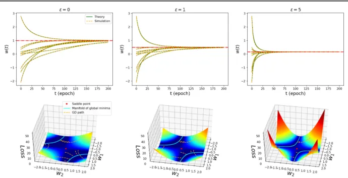
`λ= λ2(1−w2w1)2+ε2(w2w1)2withλ= 1using gradient descent. Starting from several different randomly initialised weightsw1andw2, we compare the simulated dynamics with those predicted by equation (5). The top row in Figure1 shows the exact fit between the predictions and numerical simulations for different noise levels,ε= 0,1,5.
The trajectories in the top row of Figure1converge to the optimal solution at different rates depending on the amount of injected noise. Specifically, adding more noise results in faster convergence. However, the trade-off in (4) ensures that the fixed point solution also diminishes in magnitude. To gain further insight, we also visualise the associated loss surfaces for each experiment in the bottom row of Figure1. Note that even though the scalar productw2w1defines a linear mapping, the minimisation of`λwith respect tow1 andw2 is a non-convex optimisation problem. The loss surfaces in Figure1each have an unstable saddle point at
w2=w1= 0(red star) with all remaining fixed points lying on a minimum loss manifold (cyan curve). This manifold corresponds to the different possible combinations ofw2and
w1that minimise`λ. The paths that gradient descent follow
from various initial starting weights down to points situated on the manifold are represented by dashed orange lines. For a fixed value ofλ, adding noise warps the loss surface
making steeper slopes and pulling the minimum loss mani-fold in towards the saddle point. Therefore, steeper descent directions cause learning to converge at a faster rate to fixed points that are smaller in magnitude. This is the result of a sharper curving loss surface and the minimum loss manifold lying closer to the origin.
We can compute the fixed point solution for any pair of initial starting weights (not on the saddle point) by taking
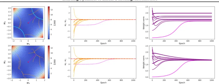
Figure 1.Learning dynamics, loss surface and gradient descent paths for linear denoising autoencoders. Top: Learning dynamics for each simulated run (dashed orange lines) together with the theoretically predicted learning dynamics (solid green lines). The red line in each plot indicates the final value of the resulting fixed point solutionw∗.Bottom: The loss surface corresponding to the loss `λ = λ2(1−w2w1)2+ ε2(w2w1)2forλ= 1, as well as the gradient descent paths (dashed orange lines) for randomly initialised
weights. The cyan hyperbolas represent the global minimum loss manifold that corresponds to all possible combinations ofw2andw1
that minimise`λ.Left:ε= 0, w∗= 1.Middle:ε= 1, w∗= 0.5.Right:ε= 5, w∗= 1/6.
the derivative d`λ dw =− λ τ(1−w) + ε τw,
and setting it equal to zero to findw∗= λ
λ+ε. This solution
reveals the interaction between the input variance associated with λand the noiseε. For large eigenvalues for which λε, the fixed point will remain relatively unaffected by adding noise, i.e.,w∗≈1. In contrast, ifλε, the noise
will result inw∗≈0. This means that over a distribution of eigenvalues, an appropriate amount of noise can help a DAE to ignore low variance directions in the input data while learning the reconstruction. In a practical setting, this motivates the tuning of noise levels on a development set to prevent overfitting.
5. The Relationship Between Noise and
Weight Decay
It is well known that adding noise to the inputs of a neural network is equivalent to a form of regularisation (Bishop, 1995). Therefore, to further understand the role of noise in linear DAEs we compare the dynamics of noise to those of explicit regularisation in the form ofweight decay(Krogh & Hertz,1992). The reconstruction loss for a linear weight
decayed autoencoder (WDAE) is given by 1 2N N X i=1 ||xi−W2W1xi||2+ γ 2 ||W1|| 2+||W 2||2 (6) whereγis the penalty parameter that controls the amount of regularisation applied during learning. Provided that the weights of the network are initialised to be small, it is also possible (see supplementary material) to derive scalar dynamics of learning from (6) as
wγ(t) = ξEγ
Eγ−1 +ξ/w0, (7)
whereξ= (1−N γ/λ)andEγ=e2ξt/τ.
Figure2compares the learning trajectories of linear DAEs and WDAEs over time (as measured in training epochs) for
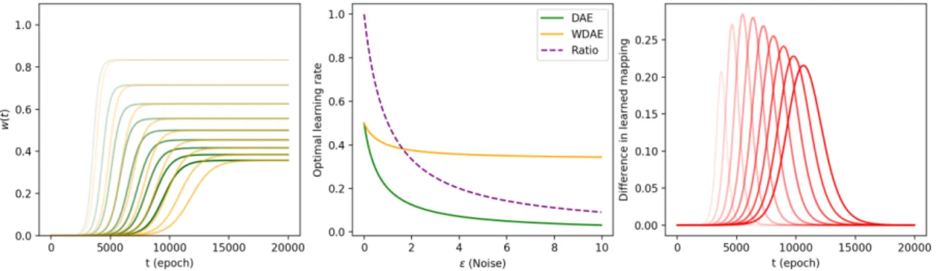
λ= 2.5,1,0.5and0.1. The dynamics for both noise and weight decay exhibit a sigmoidal shape with an initial period of inactivity followed by rapid learning, finally reaching a plateau at the fixed point solution. Figure2illustrates that the learning time associated with an eigenvalue is negatively correlated with its magnitude. Thus, the eigenvalue corre-sponding to the largest amount of variation explained is the quickest to escape inactivity during learning.
The colour intensity of the lines in Figure2correspond to the amount of noise or regularisation applied in each run,
Figure 2.Theoretically predicted learning dynamics for noise compared to weight decay for linear autoencoders.Top: Noise dynamics (green), darker line colours correspond to larger amounts of added noise.Bottom: Weight decay dynamics (orange), darker line colours correspond to larger amounts of regularisation.Left to right: Eigenvaluesλ= 2.5,1and0.5associated with high to low variance.
Figure 3.Learning dynamics for optimal discrete time learning rates (λ= 1).Left: Dynamics of DAEs (green) vs. WDAEs (orange), where darker line colours correspond to larger amounts noise or weigh decay.Middle: Optimal learning rate as a function of noiseεfor DAEs, and for WDAEs using an equivalent amount of regularisationγ=λε/(λ+ε).Right: Difference in mapping over time.
with darker lines indicating larger amounts. In the contin-uous time limit with equal learning rates, when compared with noise dynamics, weight decay experiences a delay in learning such that the initial inactive period becomes ex-tended for every eigenvalue, whereas adding noise has no effect on learning time. In other words, starting from small weights, noise injected learning is capable of providing an equivalent regularisation mechanism to that of weight decay in terms of a constrained fixed point mapping, but with zero time delay.
However, this analysis does not take into account the prac-tice of using well-tuned stable learning rates for discrete optimisation steps. We therefore consider the impact on training time when using optimised learning rates for each approach. By using second order information from the Hes-sian as inSaxe et al.(2013a), (here of the expected recon-struction loss with respect to the scalar weights), we relate the optimal learning rates for linear DAEs and WDAEs,
where each optimal rate is inversely related to the amount of noise/regularisation applied during training (see supple-mentary material). The ratio of the optimal DAE rate to that for the WDAE is
R= 2λ+γ
2λ+ 3ε. (8)
Note that the ratio in (8) will essentially be equal to one for eigenvalues that are significantly larger than bothεand γ, with deviations from unity only manifesting for smaller values ofλ.
Furthermore, weight decay and noise injected learning re-sult in equivalent scalar solutions when their parameters are related byγ= λε
λ+ε (see supplementary material). This
leads to the following two observations. First, it shows that adding noise during learning can be interpreted as a form of weight decay where the penalty parameterγadapts to each direction of variation in the data. In other words, noise essentially makes use of the statistical structure of
Figure 4.The effect of noise versus wei