Logic Programs with Annotated Disjunctions
Dimitar Shterionov, Joris Renkens, Jonas Vlasselaer, Angelika Kimmig,Wannes Meert, Gerda Janssens KULeuven, Belgium
(e-mail:[email protected])
Abstract. Probabilistic logic languages, such as ProbLog and CP-logic, are probabilistic generalizations of logic programming that allow one to model probability distributions over complex, structured domains. Their key probabilistic constructs are probabilistic facts and annotated disjunc-tions to represent binary and mutli-valued random variables, respectively. ProbLog allows the use of annotated disjunctions by translating them into probabilistic facts and rules. This encoding is tailored towards the task of computing the marginal probability of a query given evidence (MARG), but is not correct for the task of finding the most proba-ble explanation (MPE) with important applications eg., diagnostics and scheduling.
In this work, we propose a new encoding of annotated disjunctions which allows correct MARG and MPE. We explore from both theoretical and experimental perspective the trade-off between the encoding suitable only for MARG inference and the newly proposed (general) approach.
Keywords: Probabilistic Logic Programming, Statistical Relational Learning, Most Probable Explanation, Logic Programs with Annotated Disjunctions, ProbLog
1
Introduction
The field of Probabilistic Logic Programming (PLP) combines probabilistic rea-soning and logic to deal with complex relational domains. Most PLP tech-niques extend logic programming languages (such as Prolog) with probabilities. This has resulted in different probabilistic logic languages and systems, such as ProbLog [1], PRISM [2], LPADs [3], PHA [4] and others, which mostly focus on computing marginal probabilities of individual random variables or queries.
In contrast, the field of Statistical Relation Learning (SRL) often focuses on the extension of graphical models with logical and relational representations. Here, the most common inference tasks are computing the marginal probabil-ity of a set of random variables given evidence (MARG) and finding the most probable explanation given evidence (MPE).
The MPE task did not yet receive much attention in PLP, although it has important applications in diagnostics and scheduling. For a diagnostics example,
it is equivalent to finding the health state of a set of machines or components given a set of measurements. For a scheduling problem, one is interested in an optimal way of distributing resources or tasks. MPE is a special case of the computationally harder MAP (maximum a posteriori) task. The MPE is different from the task of finding the most probable proof in PLP, also called Viterbi proof [4–7], where one is interested in the proof to a query with highest probability.
ProbLog [1, 8] is a probabilistic logic and learning framework – a language and an engine. The engine handles various inference and learning tasks, including MPE inference [9], and as such tries to bridge the gap between PLP and SRL. Initially focused on probabilistic facts, or binary random variables, the ProbLog language now also supports Annotated Disjunctions (ADs) [3]. These specify exclusive choices between alternatives given some condition and thus provide an intuitive construct to represent multi-valued random variables. Internally, ProbLog encodes ADs by means of probabilistic facts and rules. However, given the semantics of ADs, this encoding is not correct for the MPE task.
In this paper, we propose an encoding of Annotated Disjunctions that is correct for both MARG and MPE inference. It uses ProbLog constraints, that is, first order logic sentences which restrict the models of ProbLog programs [10]. We compare the two encodings both theoretically and experimentally. We also incorporate an MPE inference algorithm based on weighted model counting into ProbLog.
The paper is organized as follows: In Section 2 we give background on the language ProbLog, introduce the MPE task and show why the encoding of ADs as ProbLog programs is not correct for the MPE task. Section 3 introduces our approach to encode ADs as weighted CNFs and proves its correctness. Section 4 summarizes experimental results. We conclude in Section 5.
2
Background
2.1 The ProbLog Language
The ProbLog language [1] is a probabilistic extension of Prolog. It uses proba-bilistic facts, that is, facts whose truth values are determined probaproba-bilistically to model basic uncertain data, and Prolog rules to define deterministic conse-quences of the probabilistic facts. A probabilistic fact has the form pi ::fi and states that the fact fi is true with probability true(fi) = pi, and false other-wise (with false(fi) = (1−pi)). ProbLog uses the distribution semantics [11] to define a probability distribution over the least models (orpossible worlds) of the ProbLog program. We write a possible world ω as a tuple (ω+, ω−), where
the set ω+ contains the probabilistic facts that are true andω− those that are
false, thus, omitting the (uniquely determined) truth values for non-probabilistic atoms. Treating probabilistic facts as independent binary random variables, we obtain the probability of a possible world as:
P(ω) = Y fi∈ω+ true(fi) Y fi∈ω− false(fi) (1)
Example 1. The following ProbLog program models a game with three bags with colored balls. One ball is picked from each bag, and the game is won if at least two balls are red. The probabilistic fact0.6::red(b1) states that the probability of selecting a red ball from bagb1is 0.6. It implies that selecting a ball with another color (eg. blue or green) has probability 0.4. The table outlines the set of its possible worlds (ri abbreviatesred(bi)) and their probabilities:
0.6::red(b1). 0.2::red(b2). 0.7::red(b3).
win:- red(b1), red(b2). win:- red(b2), red(b3). win:- red(b1), red(b3).
poss. worldr1r2r3 win
ω1 T T T T ω2 T T F T ω3 T F T T ω4 T F F F ω5 F T T T ω6 F T F F ω7 F F T F ω8 F F F F P(r1) P(r2) P(r3) P(ωi) 0.6 0.2 0.7 0.084 0.6 0.2 0.3 0.036 0.6 0.8 0.7 0.336 0.6 0.8 0.3 0.144 0.4 0.2 0.7 0.056 0.4 0.2 0.3 0.024 0.4 0.8 0.7 0.224 0.4 0.8 0.3 0.096
2.2 ProbLog Programs with Annotated Disjunctions
Annotated Disjunctions We recall annotated disjunctions as used in LPADs [3] and CP-Logic [12]. An annotated disjunction (AD)a is a multi-headed rule of the form p1 :: h1;. . .;pn :: hn ←b1, . . . , bm., where pi is the probability of the head atom hi, the pi sum to at most one, and the conjunction of the literals b1, . . . , bm forms the body of the AD. We denote withhead(a) the set of head
atoms of the AD a and withbody(a) the set of body literals of a. If the body is true, the AD probabilistically causes one of the head atoms to become true, otherwise the AD does not have an effect. Thus, if the same atom appears in the heads of multiple ADs, they correspond to different causes. If Pn
i=1pi <1
there is a probability (= 1−Pn
i=1pi) that none of the head atoms is caused to
be true. As this can be made explicit by adding an extra none head atom, we assume that probabilities sum to one.
We now summarize the process semantics of annotated disjunctions as defined in CP-logic; we refer to [12] for full technical details and a proof of the equivalence of this semantics with the instance based semantics of LPADs [3, 12].
Definition 1 (Probability Tree). Let A = {a1, . . . , ak} be a set of ground
annotated disjunctions over atoms LA. A probability treeT(A)is a tree where
every node n is labeled with an interpretation I(n) assigning truth values to a
subset ofLA and a probabilityP(n), constructed as follows:
– The root node ⊥has probabilityP(⊥) = 1.0 and interpretationI(⊥) ={}.
– Each inner node n is associated with an ADai such that
• no ancestor ofn is associated withai,
• all positive literals inbody(ai)are true in I(n),
• for each negative literal ¬l in body(ai), the positive literal l cannot be
made true starting from I(n).
and has one child node for each atom hj ∈ head(ai). The jth child has
interpretationI(n)∪ {hj}and probabilityP(n)·true(hj).
The path from the root to a leafnis called aselectionσnwith probabilityP(σn) =
P(n). We say that each selection defines an interpretation and denote withI(σn)
the interpretation defined by σn (I(σn) =I(n)).
All probability trees for a given set of ADs define the same distribution over selections [12]; from here on, we refer to an arbitrary probability tree when mentioning “the probability tree ofA”.
Example 2. We consider a variant of the game in Example 1 with a single bag
containing red, green and blue balls, as expressed by ADa1, where the player
randomly decides to pick a ball or not, as encoded by ADa2:
a1:0.6::red(b1); 0.3::green(b1); 0.1::blue(b1) <- pick(b1).
a2:0.6::pick(b1); 0.4::no_pick(b1) <- true.
A probability tree associated with these ADs and its selections are:
I1 = {p(b1), r(b1)} P=0.36 I2 = {p(b1), g(b1)}P=0.18 I3 = {p(b1), b(b1)}P=0.06 I4 = {np(b1)} P=0.4 {p(b1)} 0.6 0.3 0.1 {} 0.4
0.6 Selection: Interpretation Probability
P(σi)
σ1 I1 ={pick(b1),red(b1)} 0.36
σ2 I2 ={pick(b1),green(b1)} 0.18
σ3 I3 ={pick(b1),blue(b1)} 0.06
σ4 I4 ={no_pick(b1)} 0.4
Here, all selections define different interpretations.
ProbLog Encoding of Annotated Disjunctions To support MARG infer-ence for ProbLog programs with annotated disjunctions, an AD is translated to a set of probabilistic facts with suitably adapted probabilities and a Prolog rule for each of its head atoms, with bodies which are mutually exclusive. We refer to [13, Chapter 3] for the details and illustrate the principle with an example.
Example 3. The ProbLog encoding for Example 2:
0.6::pf(1, 1). 0.75::pf(1, 2). 0.6::pf(2, 1). red(b1):- pick(b1), pf(1, 1). pick(b1):- pf(2, 1). green(b1):- pick(b1), pf(1, 2), \+ pf(1, 1). no_pick(b1):- \+ pf(2, 1). blue(b1):- pick(b1), \+ pf(1, 2), \+ pf(1, 1).
2.3 Most Probable Explanations for ProbLog Programs
The inference task that has received most attention by the PLP community is computing the marginal probability of a ground query atom q given evidence E=eon a subset of the other atoms, MARG(q|E=e) =P(q|E=e). In the absence of evidence, this is also known as the success probability of a query.
In statistical relational learning (SRL) [14] and probabilistic graphical mod-els [15] one of the key tasks is to find the most likely state of the world where a set of observations (the evidence) holds, also called MPE inference. Formally, the Most Probable Explanation (MPE) task, is defined as follows.
Definition 2 (Most Probable Explanation). Given a probability
distribu-tionP(V)over a set of discrete random variablesV and a truth value assignment
e to a subset of random variablesE ⊆V (the evidence), the task of finding the
most probable explanation (MPE) is to determine a truth value assignment uto
the remaining random variables U = V \E with maximal probability, that is,
MPE(E) = arg maxuP(U =u|E =e).
A solution of the MPE task is also called an MPE state. Solution techniques de-veloped for MPE include methods based on knowledge compilation [16], integer linear programming [17], and weighted MAX-SAT [18].
For a ProbLog program without ADs, V is the set of ground atoms, E =e fixes truth values for a subset of those, and the task is to find the most likely assignment to all other atoms, that is, the possible world with the highest probability in which the evidence holds. As in [9], we assume ProbLog programs with finite groundings.
Example 4. For Example 1 given the evidencered(b2)=true the worlds where
the evidence holds areω1,ω2,ω5 andω6. The one with the highest probability
isω1. The MPE state is thus{red(b1) =true,red(b2) =true,red(b3) =true}.
For a set ofannotated disjunctionsA={a1, .., ak}, the most probable
expla-nation is the truth value assignment according to the interpretation defined by the selection in T(A) with highest probability amongst the ones for which the evidence holds. Let SE=e={σ|I(σ)|=E=e} be the set of selections in which the evidence holds and ˆσ=argmaxσ∈SE=eP(σ), thenM P EA(E) =I(ˆσ).
Example 5. For the set of ADs in Example 2, the evidence blue(b1) = false
makesσ3invalid. The MPE state given the evidence thus isσ4={no_pick(b1)}.
The ProbLog encoding of these ADs (cf. Example 3) has the following pos-sible worlds (p(b1)is short for pick(b1)andnp(b1)forno_pick(b1)):
poss. worldpf(1, 1) pf(1, 2) pf(2, 1) red(b1) green(b1) blue(b1) p(b1) np(b1)P(ωi)
ω1 T T T T F F T F 0.27 ω2 T T F F F F F T 0.18 ω3 T F T T F F T F 0.09 ω4 T F F F F F F T 0.06 ω5 F T T F T F T F 0.18 ω6 F T F F F F F T 0.12 ω7 F F T F F T T F 0.06 ω8 F F F F F F F T 0.04
The evidenceblue(b1)=false holds in all worlds exceptω7, and the MPE
state of the ProbLog program is thus {pf(1, 1) = true, pf(1, 2) = true,
pf(2, 1) =true}. For this MPE state no_pick(b1) is false and pick(b1) is
true, which is different from the MPE state of the underlying set of ADs. Example 5 illustrates that using the ProbLog encoding of annotated disjunctions can result in incorrect MPE states. The reason is that several possible worlds of the ProbLog encoding may correspond to the same selection in the probabil-ity tree. This is not a problem when computing marginal probabilities, as the probabilities of all possible worlds where the query is true are summed together.
In [9] MPE is mentioned as special case of the more general maximum a posteriori (MAP) inference. MAP is the task of finding the most likely values for a set of query atoms givenpartial evidence. The query atoms are a subset of all atoms of the ProbLog program for which evidence is not given. Solving then the MAP task requires to marginalize over the atoms which are neither given as queries nor as evidence. That is, we have to apply maximization over the query atoms given the evidence atoms and summation over the rest. MAP inference can be used in order to find the MPE state of a ProbLog program with ADs. For the ProbLog encoding of such a program we can give as queries all the atoms of that program excluding the probabilistic facts generated by the encoding. Then solving the MAP task will give the truth value assignments of these atoms which is in practice the MPE state of the initial program. The MAP inference is computationally expensive, while MPE can be computed efficiently [19, 16]. The new encoding we introduce in Section 3.1 allows to solve the MPE task on ProbLog programs with ADs both correctly and efficiently by enforcing a one-to-one correspondence between selections and possible worlds.
Relation to Most Probable Proof In PLP the term most probable
expla-nation typically is used interchangeably with most probable proof, also called
Viterbi proof [4–7]. A proof (or explanation) ω0 for a query is a partial truth
value assignment (or partial possible world) such that for all full assignments ex-tending the proof, the query holds. Finding a most likely proof (the VIT task) is different from MPE in that it does not aim at finding the state of all unobserved variables, but an assignment to a small set of variables sufficient to explain a query. More formally, given a queryq, we have V IT(q) = arg maxω0∈E(q)P(ω0)
withE(q) the set of all explanations or proofs ofq.
For certain types of models, finding the Viterbi proof for queryqcorresponds to solving MPE withq=trueas evidence. This is true for instance in programs modeling Hidden Markov Models, where both VIT and MPE have to make one choice per time point, but does not hold in general:
Example 6. In the program below, query win has two proofs: the first uses
facts red and green and has probability 0.4 ·0.9 = 0.36, the second uses facts blue and yellow and has probability 0.5·0.6 = 0.3. The Viterbi proof for win is the first one. The MPE state for evidence win = true, however, is
{¬red,green,blue,yellow}. This state does not extend the Viterbi proof.
0.4::red. 0.9::green. win :- red, green. 0.5::blue. 0.6::yellow. win :- blue, yellow.
Relation to Most Probable Explanation for Bayesian Networks To encode a Bayesian network using Annotated Disjunctions, each row in each con-ditional probability table (CPT) is encoded as a deterministic rule to capture the value assignments and a probabilistic fact to capture the probability. There is only one CPT per variable (the child node) and the rows in a CPT express mutually exclusive value assignments to a set of variables (the parents of the node). For each value assignment to the parents we introduce one AD with head
atoms encoding the different value assignments to the child node and body as-sociated to the value of the parents. The probability of each head atom is the probability given in the CPT for the value assignment of the parents. It has been shown that this encoding with ADs expresses the same probability distribution as the Bayesian network [20].
It can be shown that, given Definition 2, the MPE state of the Bayesian network is equivalent to the MPE state of a set of ADs that encode the Bayesian network. The probability tree inferred by a set of ADs that encode a Bayesian network has as property that each leaf has a unique interpretation. Therefore, the interpretation with the highest probability and the selection with the highest probability are equivalent. An intuitive proof can be constructed as follows: For any given CPT for a variable a, at each point in constructing the probability tree, if all parent variables of a certain CPT are present in the current partial interpretation, exactly one rule withaas head has a condition that is true. For each value ofaa subtree is instantiated. None of the other rules can have a true condition in any of the subtrees due to the mutually exclusivity. This guarantees that each subtree has a different value assigned toaand no two interpretations in different subtrees can be identical.
3
Weighted CNF Encoding for Annotated Disjunctions
ProbLog inference is based on a transformation of the ProbLog program to a weighted Boolean formula in CNF, on which weighted model counting (WMC) is used to compute probabilities [8]. We now introduce a new encoding of annotated disjunctions in line with this transformation and consistent for MPE.
3.1 Encoding
The encoding of annotated disjunctions we propose (which we refer to as the
WMC encoding to differentiate it from theProbLog encoding discussed in Sec-tion 2.2.) has two parts: (i) a logic program with weighted facts that is trans-formed to CNF as in ProbLog; (ii) a set of constraints that is directly added to the weighted CNF. This is a special case of ProbLog with constraints (cProbLog) [10], adapted directly to the specific constraints needed here. ProbLog employs weighted model counting (WMC) techniques for MARG and MPE inference on the weighted CNF.
Definition 3 (WMC encoding for ADs). The WMC encoding of a ground AD p1::h1;..;pn::hn ←b1, .., bm. with unique identifieraj consists of:
– for each hi with 1≤i≤n a surrogate probabilistic fact spf(aj,hi,i) with
true(spf(aj,hi,i)) =pi and false(spf(aj,hi,i)) = 1.0 and a clause hi:−b1, ..,bm,spf(aj,hi,i).
– (the conjunction of ) the following two constraints: n−1 ^ i=1 n ^ l=i+1 (¬spf(aj,hi,i)∨ ¬spf(aj,hl,l)), m ^ k=1 bk ↔ n _ i=1 spf(aj,hi,i)
Intuitively, surrogate probabilistic facts make the choices in ADs explicit, and constraints ensure that this does not introduce undesired combinations of values. When one head atomhiis selected for an AD, the other head atoms are ignored. That is, they do not influence the probability of any selections withhitrue. That is why the false probability of a surrogate probabilistic fact is set to 1.0. The first constraint states that for each AD, at most one surrogate probabilistic fact can be true in any possible world, and thus only one head atom can be made true by the AD. The second constraint states that a choice is made if and only if the body of the AD is true. We write a surrogate probabilistic factspf(aj,hi,i) withtrue(spf(aj,hi,i)) =pas (p,1.0) ::spf(aj,hi,i).
Example 7. The WMC encoding of the two ADs of Example 2 consists of the
program part:
(0.6, 1.0)::spf(1, red(b1), 1). blue(b1):- pick(b1), spf(1, blue(b1), 3). (0.3, 1.0)::spf(1, green(b1), 2). (0.6, 1.0)::spf(2, pick(b1), 1). (0.1, 1.0)::spf(1, blue(b1), 3). (0.4, 1.0)::spf(2, no_pick(b1), 2). red(b1):- pick(b1), spf(1, red(b1), 1). pick(b1):- spf(2, pick(b1), 1). green(b1):- pick(b1), spf(1, green(b1), 2). no_pick(b1):- spf(2, no_pick(b1), 2).
and the four constraints where in the last one we omit the equivalence with
true:
(¬spf(1,red(b1),1)∨ ¬spf(1,green(b1),2))∧(¬spf(1,red(b1),1)∨ ¬spf(1,blue(b1),3))∧ (¬spf(1,green(b1),2)∨ ¬spf(1,blue(b1),3))
pick(b1)↔(spf(1,red(b1),1)∨spf(1,green(b1),2)∨spf(1,blue(b1),3)) ¬spf(2,pick(b1),1)∨ ¬spf(2,no pick(b1),2)
spf(2,pick(b1),1)∨spf(2,no pick(b1),2)
The possible worlds of the program part in which the constraints hold are (r,g,
b,p,npabbreviatered(b1),green(b1),blue(b1),pick(b1),no_pick(b1)):
poss. worldspf(1,r,1) spf(1,g,2) spf(1,b,3) spf(2,p,1) spf(2,np,2) r g b p npP(ωi) ω1 T F F T F T F F T F 0.36 ω2 F T F T F F T F T F 0.18 ω3 F F T T F F F T T F 0.06 ω4 F F F F T F F F F T 0.40 3.2 Correctness
Theorem 1. For a setA={a1, . . . , ak}of ground annotated disjunctions, there
is a bijection from the setM of models of the weighted CNF forAto the setS
of selections in a probability tree T forA.
Proof.Let LA be the set of atoms inA, andLF the set of surrogate facts in the
weighted CNF encoding ofA. For every truth value assignment lF toLF, there
is exactly one truth value assignmentlA toLAsuch that lF∪lAis a model of the
program part of the encoding [9]. The first constraint filters out all assignments
and the second filters out those that assign true to any surrogate fact for an AD
whose body is false inlF∪lA. Each remaining assignmentlF∪lAis in one-to-one
correspondence with a selection in S. That is, each such an assignment (i.e. a
model) corresponds to exactly one path from the root to a leaf of the treeT (the
assignment lA is a model of the node’s interpretation) and there is one model
for each path.
Theorem 2. Given a set A = {a1, . . . , ak} of ground annotated disjunctions,
the set Mof models of the weighted CNF for A, and the set S of selections in
a probability tree T forA, the weight of a model M ∈M equals the probability
of the corresponding selection S∈S.
Proof. Follows directly from the fact that the model and the selection follow the same path through the tree and the definition of the weight function on the CNF. At each node, the probability of the selection so far is multiplied with the
probability pi of the chosen head atom, and the weight of the model with the
weight of the AD’s surrogate facts, pi·1.0·. . .·1.0 =pi.
Theorems 1 and 2 proof that our approach mirrors exactly the semantics of annotated disjunctions into ProbLog programs with FOL constraints. Example 8 illustrates the generality of our approach by encoding ADs which have the same atoms in their heads, i.e. the same event can result from multiple causes.
Example 8. Consider again the same problem as in the previous examples: a bag
with colored balls. According to one source of information in the bag there are red, green and blue balls (as in Example 2); another source states that there are only red and green balls in the bag. This knowledge is expressed by the following program:
r1:0.6::red(b1); 0.3::green(b1); 0.1::blue(b1) <- pick(b1).
r2:0.7::red(b1); 0.3::green(b1) <- pick(b1).
r3:0.6::pick(b1); 0.4::no_pick(b1) <- true.
The probability tree associated with these ADs is:
I2 = {p(b1), r(b1), r(b1)} ={p(b1), r(b1)} P=0.252 I3 = {p(b1), r(b1), g(b1)} P=0.234 I4 = {p(b1), g(b1), g(b1)} ={p(b1), g(b1)} P=0.054 I5 = {p(b1), b(b1), r(b1)} P=0.042 {p(b1)} I6 = {p(b1), b(b1), g(b1)} P=0.018 I1 = {np(b1)} P=0.4 {p(b1), r(b1)} 0.6 {p(b1), g(b1)} 0.3 {p(b1), b(b1)} 0.1 0.7 0.3 0.7 0.3 0.7 0.3 {} 0.4 0.6
Selection: Interpretation Probability
P(σi)
σ1 I1 ={no_pick(b1)} 0.4
σ2 I2 ={pick(b1),red(b1)} 0.252
σ3 I3 ={pick(b1),red(b1),green(b1)} 0.108
σ4 I3 ={pick(b1),red(b1),green(b1)} 0.126
σ5 I4 ={pick(b1),green(b1)} 0.054
σ6 I5 ={pick(b1),red(b1),blue(b1)} 0.042
σ7 I6 ={pick(b1),green(b1),blue(b1)} 0.018
Picking from the bag can result in selecting a red or green ball or red, green or blue ball (according to the different sources of information). In this case there are two selections (σ2 andσ3) which define the same interpretation (I2). When
computing the MPE (as defined in Definition 2), each of these selections should be considered separately. The following table shows that our method corresponds exactly one possible world to each selections, regardless if they have the same interpretation and thus the MPE state can be computed correctly.
Possible pf(1, r) pf(1, g) pf(1, b) pf(2, r) pf(2, g) pf(3, p) pf(3, np) r g b p np Probability World P(ωi) ω1 F F F F F F T F F F F T 0.4 ω2 T F F T F T F T F F T F 0.252 ω3 F T F T F T F T T F T F 0.108 ω4 F F T T F T F T F T T F 0.126 ω5 T F F F T T F T T F T F 0.054 ω6 F T F F T T F F T F T F 0.042 ω7 F F T F T T F F T T T F 0.018
4
Evaluation
4.1 AnalysisThe ProbLog pipeline for both MARG and MPE inferences consists of
Ground-ing,CNF conversion,sd-DNNF compilation andEvaluationstages. Each
previ-ous stage produces input for the next one. ADs are processed in the Grounding stage. Using the ProbLog encoding the grounder generates only a ground pro-gram. On the other hand, invoking the WMC encoding results in (i) a ground program and (ii) CNF (ϕADs) of the constraints to preserve the semantics of the ADs. In the second stage the ground program is converted to a (weighted) CNF formulaϕg. For the WMC encoding the CNF conversion generates the formula ϕ=ϕg∧ϕADs∧ϕE, whereϕEis the CNF that states that the evidence (if any given) should hold (for the ProbLog encoding it isϕ=ϕg∧ϕE).
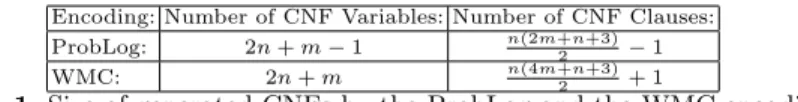
For an AD with|head|=nand |body|=mthe corresponding ProbLog en-coding has n rules, with thenth rule containing m+n−1 facts in its body. The WMC encoding constructs rules with constant body size (m+ 1). Table 1 compares the number of variables and clauses in the CNFϕgenerated from the different encodings of an AD which does not introduce cycles. It shows that the ProbLog encoding produces smaller CNFs as compared to the WMC Encod-ing. Both encodings deal with each AD independently and define one (ground ProbLog) rule for each dependency between a head atom and the probabilistic facts generated by the encoding. The bodies of rules with the same head are combined in a disjunction in the CNF and introduce additional variables and clauses. For the two encodings of a set of ADs which share head atoms the num-ber of additional variables and clauses in the CNF is the same. ProbLog employs
Encoding: Number of CNF Variables: Number of CNF Clauses:
ProbLog: 2n+m−1 n(2m+2n+3)−1
WMC: 2n+m n(4m+2n+3)+ 1
Table 1.Size of generated CNFs by the ProbLog and the WMC encoding.
the algorithm of [21] to break cycles. It has the same impact on both encodings. Table 1 ignores the additional clauses and variables in the cases where the ADs share head atoms and the ones introduced during loop breaking as they are the same for both encodings.
The sd-DNNF compilation stage is computationally the hardest in the pipeline of ProbLog. We use c2d [22] to compile a CNF into a sd-DNNF. c2d is non-deterministic (cf. [23]), that is, for the same CNF the resulting sd-DNNFs may differ. Hence, we cannot make theoretical estimations on the time for generating an sd-DNNF, its size or the time for its evaluation.
Our implementation of the evaluation procedure for the MPE task is accord-ing to [16, Chapter 12] and has the same complexity as the evaluation for the MARG task. Our experiments confirmed this claim.
4.2 Experimental Data
Our experiments aim to answer: (i) What is the trade-off between the ProbLog encoding and the WMC encoding when doing MARG infer-ence?;(ii) How does the WMC encoding scale w.r.t. the data size?.
We analyze the results from experimenting on three artificially generated datasets. The first one (the Balls benchmark) is a more complex version of the ball game (cf. Example 2) that uses ADs to represent the different possible consequences of an action. The two other benchmarks are taken from [24]: we use the programs with annotated disjunctions with increasing head atoms (Mgh) and the ones with increasing number of (negated) body atoms (Mgnb). With the Mgh dataset we show the impact of the number of heads on the performance of the encodings. TheMgnb dataset shows the impact of the size of the bodies (that is, the second constraint of the WMC encoding). Our benchmarks can be found atpeople.cs.kuleuven.be/~dimitar.shterionov/mpe.
To assess the performance of our approach we measure theprocessing-compilation
time (time for grounding plus CNF conversion plus sd-DNNF compilation), the evaluation time and the total inference time. We report the ratioTr= T(P robLog)
T(W M C)
per number of ground ADs which shows the relative time between the ProbLog and the WMC encoding. To assess the memory consumption we compare the number of nodes and edges for the generated sd-DNNF in each test run. We report the size ratioSr= S(P robLog)
S(W M C) .
Since c2d may generate different sd-DNNFs for the same CNF we run each test 5 times and report the average of time and size. We run our experiments on an 8-thread, IntelrCoreTMi7 @ 3400 MHz machine with 16GB RAM.
4.3 Experimental Results
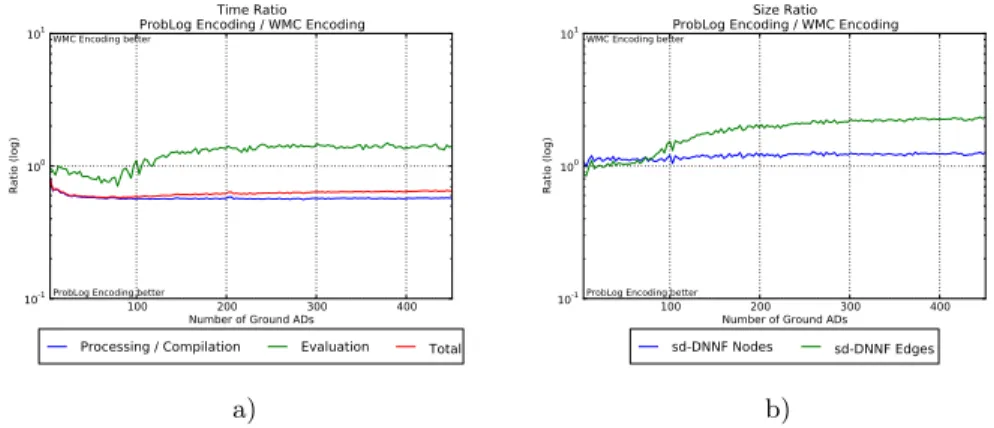
Figure 1 summarizes the results for theBalls program. Figure 1 a) shows the time ratioTrw.r.t. the number of ADs and Figure 1 b) the size ratioSr.
100 200 300 400
Number of Ground ADs 10-1
100
101
Ratio (log)
ProbLog Encoding better WMC Encoding better
Time Ratio ProbLog Encoding / WMC Encoding
Processing / Compilation Evaluation Total
a)
100 200 300 400
Number of Ground ADs 10-1
100
101
Ratio (log)
ProbLog Encoding better WMC Encoding better
Size Ratio ProbLog Encoding / WMC Encoding
sd-DNNF Nodes sd-DNNF Edges
b)
Fig. 1.Results from theBallsbenchmark.
Figure 1 a) shows a worse processing-compilation time (blue line) for the WMC encoding compared to the ProbLog encoding but better evaluation time (green line). Since the processing-compilation time is much larger than the evalu-ation, the total time (red line) is also worse for the WMC encoding. Furthermore, the total time for the case of the WMC encoding is higher (as compared to the ProbLog encoding) with a constant factor over the number of ground ADs.
From Figure 1 b) we conclude that for almost all queries the compiled sd-DNNFs for the WMC encoding are smaller. This, together with the better eval-uation time shows the WMC encoding to be preferable, since e.g., in diagnostics typically the model is compiled once and evaluated many times.
The results from experimenting on theMghdataset, summarized in Figure 2, show similar tendencies as the ones for theBallsbenchmark. That is, the WMC encoding has worse processing-compilation and therefore also total execution time but still better evaluation time. Crucial for the encoding is the size of the body of the AD as it influences drastically the size of the CNF (cf. Table 1). Figure 3 shows how this affects the execution time. For the Mgnb dataset the WMC encoding results in worse processing-compilation, total and evaluation time than the ProbLog encoding.
Analyzing the results of our experiments we can state that there is a trade-off between the ProbLog encoding and the WMC encoding: generally, the total execution time for inference is worse (for the WMC encoding case). But the better evaluation time (BallsandMghbenchmarks) due to the more compact sd-DNNFs makes our encoding preferable for problems where you compile once and evaluate many times. Also, in extreme cases, like theMgnbbenchmark, the WMC encoding does not perform better. Our experiments also show that with the two
4 6 8 10 12 14 Number of Ground ADs
10-1
100
101
Ratio (log)
ProbLog Encoding better WMC Encoding better
Time Ratio ProbLog Encoding / WMC Encoding
Processing / Compilation Evaluation Total
a)
4 6 8 10 12 14
Number of Ground ADs 10-1
100
101
Ratio (log)
ProbLog Encoding better WMC Encoding better
Size Ratio ProbLog Encoding / WMC Encoding
sd-DNNF Nodes sd-DNNF Edges
b)
Fig. 2.Results from theMgh benchmark.
10 20 30 40 50
Number of Ground ADs 10-1
100
101
Ratio (log)
ProbLog Encoding better WMC Encoding better
Time Ratio ProbLog Encoding / WMC Encoding
Processing / Compilation Evaluation Total
a)
10 20 30 40 50
Number of Ground ADs 10-1
100
101
Ratio (log)
ProbLog Encoding better WMC Encoding better
Size Ratio ProbLog Encoding / WMC Encoding
sd-DNNF Nodes sd-DNNF Edges
b)
Fig. 3.Results from theMgnbbenchmark.
encodings ProbLog’s inference scales in similar ways, with the ProbLog encoding outperforming the WMC encoding with respect to total execution time.
5
Conclusion
In this paper we introduced an encoding of annotated disjunctions as a weighted CNF formula (theWMC Encoding) to correctly reason with annotated disjunc-tions within the ProbLog system. ADs were supported previously by transform-ing them into probabilistic facts and Prolog rules. This approach (theProbLog
encoding) was correct for the MARG task but not for the MPE task. We showed
that the WMC Encoding is correct both for the MARG and the MPE tasks. We then compared its performance to the ProbLog encoding with respect to MARG inference. Our new encoding is preferable for MPE inference and MARG in-ference with more than one evaluation (as it is the case for e.g. diagnostics
problems). While for the typical MARG task, the ProbLog encoding is better.
References
1. De Raedt, L., Kimmig, A., Toivonen, H.: ProbLog: a probabilistic Prolog and its application in link discovery. In: Proceedings of the 20th International Joint Conference on Artificial Intelligence, AAAI Press (2007) 2468–2473
2. Sato, T., Kameya, Y.: Parameter learning of logic programs for symbolic-statistical modeling. Journal of Artificial Intelligence Research15(2001) 391–454
3. Vennekens, J., Verbaeten, S., Bruynooghe, M.: Logic programs with annotated disjunctions. In: Proceedings of International Conference on Logic Programming, Springer (2004) 431–445
4. Poole, D.: Logic programming, abduction and probability. New Generation Com-puting11(1993) 377–400
5. Sato, T., Kameya, Y.: A viterbi-like algorithm and EM learning for statistical abduction. In: Proceedings of Workshop on Fusion of Domain Knowledge with Data for Decision Support. (2000)
6. Kimmig, A., Demoen, B., De Raedt, L., Santos Costa, V., Rocha, R.: On the implementation of the probabilistic logic programming language ProbLog. Theory and Practice of Logic Programming11(2011) 235–262
7. Bragaglia, S., Riguzzi, F.: Approximate inference for logic programs with annotated disjunctions. In: Revised papers of ILP 2010. (2011) 30–37
8. Fierens, D., Van Den Broeck, G., Renkens, J., Shterionov, D., Gutmann, B., Thon, I., Janssens, G., De Raedt, L.: Inference and learning in probabilistic logic programs using weighted boolean formulas. Theory and Practice of Logic Programming (2014) accepted, http://arxiv.org/abs/1304.6810.
9. Fierens, D., Van den Broeck, G., Thon, I., Gutmann, B., De Raedt, L.: Inference in probabilistic logic programs using weighted CNF’s. In: Proceedings of the 27th Conference on Uncertainty in Artificial Intelligence. (2011) 211–220
10. Fierens, D., Van den Broeck, G., Bruynooghe, M., De Raedt, L.: Constraints for probabilistic logic programming. In Roy, D., Mansinghka, V., Goodman, N., eds.: Proceedings of the NIPS Probabilistic Programming Workshop. (2012)
11. Sato, T.: A statistical learning method for logic programs with distribution seman-tics. In: Proceedings of the 12th International Conference on Logic Programming (ICLP95), MIT Press (1995) 715–729
12. Vennekens, J., Denecker, M., Bruynooghe, M.: CP-logic: A language of causal probabilistic events and its relation to logic programming. Theory and Practice of Logic Programming 9(2009) 245–308
13. Gutmann, B.: On Continuous Distributions and Parameter Estimation in Proba-bilistic Logic Programs. PhD thesis, KULeuven (2011)
14. Getoor, L., Taskar, B.: Introduction to Statistical Relational Learning (Adaptive Computation and Machine Learning). MIT Press (2007)
15. Koller, D., Friedman, N.: Probabilistic Graphical Models: Principles and Tech-niques. MIT Press (2009)
16. Darwiche, A.: Modeling and Reasoning with Bayesian Networks. Cambridge Uni-versity Press (2009) Chapter 12.
17. Taskar, B., Guestrin, C., Koller, D.: Max-margin markov networks. In: Proceedings of Neural Information Processing Systems. (2003)
18. Richardson, M., Domingos, P.: Markov logic networks. Machine Learning62(1-2) (2006) 107–136
19. Huang, J.: Solving map exactly by searching on compiled arithmetic circuits. In: Proceedings of the 21st National Conference on Artificial Intelligence (AAAI-06. (2006) 143–148
20. Meert, W.: Inference and Learning for Directed Probabilistic Logic Models. PhD thesis, Informatics Section, Department of Computer Science, Faculty of Engineer-ing Science (2011) Blockeel, Hendrik (supervisor).
21. Mantadelis, T., Janssens, G.: Dedicated tabling for a probabilistic setting. In Hermenegildo, M.V., Schaub, T., eds.: ICLP (Tech. Communications). Volume 7 of LIPIcs., Schloss Dagstuhl - Leibniz-Zentrum fuer Informatik (2010) 124–133 22. Darwiche, A.: New advances in compiling CNF into decomposable negation normal
form. In: Proceedings of the 16th European Conference on Artificial Intelligence. (2004) 328–332
23. Darwiche, A.: A compiler for deterministic, decomposable negation normal form. In Dechter, R., Sutton, R.S., eds.: AAAI/IAAI, AAAI Press/MIT Press (2002) 627–634
24. Meert, W., Struyf, J., Blockeel, H.: CP-logic theory inference with contextual variable elimination and comparison to BDD based inference methods. In: Proc. 19th International Conf. of Inductive Logic Programming. (2009) 96–109