Markov blanket: efficient strategy for feature subset selection method for high dimensionality microarray cancer datasets

Markov Blanket: Efficient Strategy for Feature Subset Selection

Method for High Dimensionality Microarray Cancer Datasets

by

Abdala Nour

A thesis submitted in partial fulfillment

of the requirements for the degree of

Master of Science (MSc) in Computational Sciences

The Faculty of Graduate Studies

Laurentian University

Sudbury, Ontario, Canada

ii THESIS DEFENCE COMMITTEE/COMITÉ DE SOUTENANCE DE THÈSE

Laurentian Université/Université Laurentienne Faculty of Graduate Studies/Faculté des études supérieures Title of Thesis

Titre de la thèse Markov Blanket: Efficient Strategy for Feature Subset Selection Method for High Dimensionality Microarray Cancer Datasets

Name of Candidate

Nom du candidat Nour, Abdala

Degree Diplôme Master of Science

Department/Program Date of Defence

Département/Programme Computational Sciences Date de la soutenance August 28, 2017

APPROVED/APPROUVÉ Thesis Examiners/Examinateurs de thèse:

Dr. Kalpdrum Passi

(Supervisor/Directeur de thèse) Dr. Ratvinder Grewal

(Committee member/Membre du comité) Dr. Mazen Saleh

(Committee member/Membre du comité)

Approved for the Faculty of Graduate Studies Approuvé pour la Faculté des études supérieures Dr. David Lesbarrères

Monsieur David Lesbarrères Dr. Sanjeena Dang Dean, Faculty of Graduate Studies (External Examiner/Examinateur externe) Doyen, Faculté des études supérieures

ACCESSIBILITY CLAUSE AND PERMISSION TO USE

I, Abdala Nour, hereby grant to Laurentian University and/or its agents the non-exclusive license to archive and make accessible my thesis, dissertation, or project report in whole or in part in all forms of media, now or for the duration of my copyright ownership. I retain all other ownership rights to the copyright of the thesis, dissertation or project report. I also reserve the right to use in future works (such as articles or books) all or part of this thesis, dissertation, or project report. I further agree that permission for copying of this thesis in any manner, in whole or in part, for scholarly purposes may be granted by the professor or professors who supervised my thesis work or, in their absence, by the Head of the Department in which my thesis work was done. It is understood that any copying or publication or use of this thesis or parts thereof for financial gain shall not be allowed without my written permission. It is also understood that this copy is being made available in this form by the authority of the copyright owner solely for the purpose of private study and research and may not be copied or reproduced except as permitted by the copyright laws without written authority from the copyright owner.

iii

Abstract

Currently, feature subset selection methods are very important, especially in areas of application for which datasets with tens or hundreds of thousands of variables (genes) are available. Feature subset selection methods help us select a small number of variables out of thousands of genes in microarray datasets for a more accurate and balanced classification.

Efficient gene selection can be considered as an easy computational hold of the subsequent classification task, and can give subset of gene set without the loss of classification performance. In classifying

microarray data, the main objective of gene selection is to search for the genes while keeping the maximum amount of relevant information about the class and minimize classification errors. In this paper, explain the importance of feature subset selection methods in machine learning and data mining fields. Consequently, the analysis of microarray expression was used to check whether global biological differences underlie common pathological features in different types of cancer datasets and identify genes that might anticipate the clinical behavior of this disease. Using the feature subset selection model for gene expression contains large amounts of raw data that needs analyzing to obtain useful information for specific biological and medical applications. One way of finding relevant (and removing redundant ) genes is by using the Bayesian network based on the Markov blanket [1]. We present and compare the performance of the different approaches to feature (genes) subset selection methods based on Wrapper and Markov Blanket models for the five-microarray cancer datasets. The first way depends on the Memetic algorithms (MAs) used for the feature selection method. The second way uses MRMR(Minimum Redundant Maximum Relevant) for feature subset selection hybridized by genetic search optimization techniques and afterwards compares the Markov blanket model’s performance with the most common classical classification

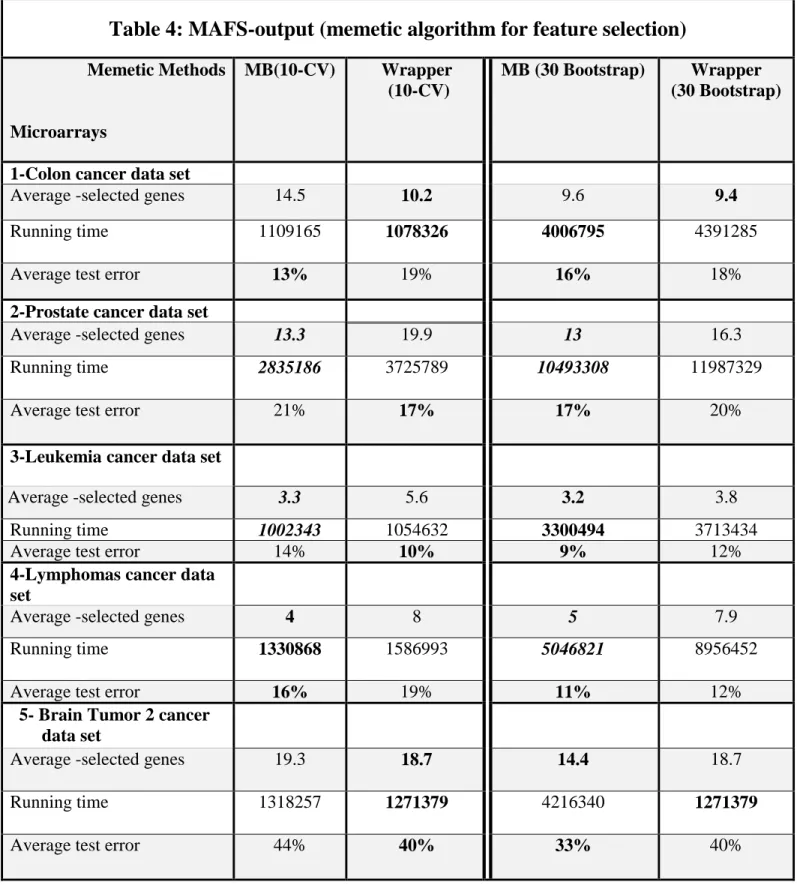
iv For the memetic algorithm, we present a comparison between two embedded approaches for feature subset selection which are the wrapper filter for feature selection algorithm (WFFSA) and Markov Blanket

Embedded Genetic Algorithm (MBEGA). The memetic algorithm depends on genetic operators (crossover, mutation) and the dedicated local search procedure. For comparisons, we depend on two evaluations techniques for learning and testing data which are 10-Kfold cross validation and 30-Bootstraping. The results of the memetic algorithm clearly show MBEGA often outperforms WFFSA methods by yielding more significant differentiation among different microarray cancer datasets.

In the second part of this paper, we focus mainly on MRMR for feature subset selection methods and the Bayesian network based on Markov blanket (MB) model that are useful for building a good predictor and defying the curse of dimensionality to improve prediction performance. These methods cover a wide range of concerns: providing a better definition of the objective function, feature construction, feature ranking, efficient search methods, and feature validity assessment methods as well as defining the relationships among attributes to make predictions.

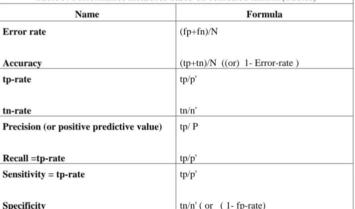
We present performance measures for some common (or classical) learning classification algorithms (Naive Bayes, Support vector machine [LiBSVM], K-nearest neighbor, and AdBoostM Ensampling) before and after using the MRMR method. We compare the Bayesian network classification algorithm based on the Markov Blanket model’s performance measure with the performance of these common classification

algorithms. The result of performance measures for classification algorithm based on the Bayesian network of the Markov blanket model get higher accuracy rates than other types of classical classification algorithms for the cancer Microarray datasets.

Bayesian networks clearly depend on relationships among attributes to make predictions. The Bayesian network based on the Markov blanket (MB) classification method of classifying variables provides all necessary information for predicting its value. In this paper, we recommend the Bayesian network based on

v the Markov blanket for learning and classification processing, which is highly effective and efficient on feature subset selection measures.

Keywords

Microarray datasets, feature selection methods, genetic algorithms, memetic algorithms,overfitting

problem, fitness function, crossover, mutation, Markov Blanket, minimum redundancy-maximum relevant, support vector machine, naive Bayes, k-nearest-neighbor, ensemble classifier, Bayesian networks.

Acknowledgements

First and foremost, I would like to acknowledge the tireless and prompt help of my supervisor in the Computational Science division at Laurentian University, Dr. Kalpdrum Passi, who has allowed me complete freedom to define and explore my own directions in research. I thank him for his consistent support and encouragement through all stages of my master’s study. Dr. Passi was always kind and positive with me even when I faced problems during my study, which has given me confidence to complete this work.

In addition to Dr. Passi, I am deeply grateful for all the staff of my Computational Science department. They have provided me with very much appreciated knowledge and information during my study and they have kindly given me teaching assistantship positions during my study.

Special thanks must also go to all my family and friends in Canada. They have provided unconditional support and encouragement through both the highs and lows of my time in graduate school.

vi

Table of Contents

1.1 INTRODUCTION TO MACHINE LEARNING ... 1

1.2 GENE EXPRESSIONS AND MICROARRAYS ... 1

1.3 MOTIVATION ... 4

1.4 ORGANIZATION ... 6

CHAPTER 2 ... 7

LITERATURE REVIEW ... ERROR! BOOKMARK NOT DEFINED.7 2.1 NAÏVE BAYES CLASSIFIER ……….7

2.2 SUPPORT VECTOR MACHINE ……….9

2.2.1 SVM NOTATIONs AND TERMINOLOGY ………9

2.2.2 OPTIMAL HYPERPLANE ………..………11

2.2.3 LINEAR SEPARABLE OF SVM ……….….…11

2.3 K-NEAREST NEIGHBORs ……….……….……16

2.3.1 DISTANCE FUNCTIONS ………..……….…18

2.3.2 SIZE OF K AND OVERFITTING PROBLEM ……….………19

2.4 ENSEMBLE CLASSIFIER ………..………20

2.5 BAYESIAN NETWORK ……….………23

vii

2.5.2 V-STRUCTURE ………..……….26

2.5.3 D-SEPARATION ………26

CHAPTER 3 ... 27

FEATURE SELECTION METHODS ... 27

3.1GOALSOFFEATURE SELECTION ... 27

3.2FEATURE SELECTION CATEGORIZE ... 27

3.3 FEATURERELEVANCEANDREDUNDANCY ... 30

3.3.1FEATURERELEVANCE ... 30

3.3.2FEATUREREDUNDANCY ... ERROR!BOOKMARK NOT DEFINED.31 3.4INTRODUCTIONTOMARKOVBLANKET ... 32

3.5A CORRELATION BASED METHOD ... 39

3.6ENTROPYANDMUTUALINFORMATION ... 39

3.7EVOLUTIONARYANDMEMETICALGORITHMFORFEATURESELECTION……….…41

3.7.1GENETIC ALGORITHM ... 43

3.7.2GENETIC ALGORITHM OPERATORS ... 43

CHAPTER 4 ... 45

METHODOLOGY ... 45

4.1 MEMETIC ALGORITHM REPRESENTATION AND OPERATORS ... 45

4.1.1 PARAMETER SETTINGS ... 46

4.1.2 OBJECTIVE FUNCTION AND FITNESS EVALUATION ... 47

4.1.3 LOCAL IMPROVEMENT OFFSPRING FUNCTION ... ..Error! Bookmark not defined.47 4.2 MRMR FOR FEATURE SELECTION ... 49

viii

DATA SETS AND EVALUATION PROCESS ... 52

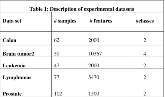
5.1 DATA SETS ... 52

5.2 ESTIMATING PREDICTION ERRORS ... 53

5.2.1 10-fold cross validation ... 53

5.2.2 BOOTSTRAP ... 53

5.3 EVALUATED METHODS ... 54

CHAPTER 6 ... ERROR! BOOKMARK NOT DEFINED.56 RESULTS AND DISCUSSION ... 56

6.1 RESULTS ... Error! Bookmark not defined.56 6.2 DISCUSSION ... 56

CHAPTER 7 ... 62

CONCLUSIONS ... 62

1

Chapter 1

Introduction

1.1 Introductionto machine learning

Machine learning is a branch of artificial intelligence using a set of algorithms to build analytical models, help computers “learn,” and find patterns in data. It can be applied to high dimensionality data to create exciting new applications and more accurately predict outcomes without being explicitly programmed. Moreover, machine learning is said to allow learning whether performance on a defined task (or tasks) will improve with experience. More specifically, machine learning can modify algorithms and subsequently do the same task (or tasks) more efficiently [2, 3].

In many cases, to improve the performance of learning algorithms in a supervised learning machine, feature subset selection is considered an underlying obstacle to defining the perfect model. Feature subset selection techniques help reduce noisy or irrelevant genes before applying the classification algorithm. Also, it improves the performance measure of learning classification algorithms[2].

1.2 Gene Expressions and Microarrays

DNA microarray technology is a powerful new research tool capable of an expression level of one thousand to ten thousand genes, each representing a different gene in an organism. Microarrays are used to analyze the gene expression levels in two different populations of cells (e.g., to look at gene expression in plants grown under different conditions, to look at gene expression in normal cells vs. cancer cells). This is done by labeling cDNAs from two different groups of cells with two different dyes and

2 hybridizing them to the microarrays. Genes are “differentially regulated,” meaning all cells in an

organism contain the same genes, but different genes are expressed (transcribed) in different tissues under

different conditions. This gives different tissues their different phenotypes, or appearance and function. DNA microarray can measure gene sequencing expression, DNA transcription, and hybridization to analyze and identify thousands of genes simultaneously. Gene expression microarrays can be used to select which genes increase or decrease activities, also referred to as transcriptional profiles or gene expression “signatures” that have since established distinct tumor types. They also allow us to determine which genes are active in different cell states. Furthermore, studying and analyzing gene expression in normal and tumor tissues will help researchers identify genes or groups of genes expressed to understand gene regulation, genetic mechanisms of disease, and function as well as response to drug treatment [4]. We can obtain gene expression data by using high-throughput technologies such as microarray and oligonucleotide chips in different tissues. Raw microarray data are images which must be transformed into gene expression matrices (or tables) where the rows represent genes’ expression patterns, the columns represent various sample types such as tissues or experimental conditions, and each cell characterizes the particular gene’s measured expression level in a sample [5, 6]. When we have gene expression data,

annotation can be added either to the gene or to the sample. For example, the gene’s function or additional details on the biology of the sample can be provided, such as “cancer state” or

“normal state” [7]. There are two straightforward methods used to study the gene expression matrix:

1. comparing gene expression profiles by comparing rows in the expression matrix; 2. comparing sample expression profiles by comparing columns in the matrix.

Additionally, by studying the gene expression matrix (data) we can look for similarities and differences between genes (or samples). If the two genes are similar, we can emphasize clues that

3 they are co-regulated and possibly functionally related. By comparing samples, we can find which genes are differentially expressed in different situations [8].

Moreover, due to the high dimensionality (curse dimensionality) of microarray datasets, they often contain many irrelevant and redundant features which increase the complexity of classification and influence the performance of most learning algorithms [9]. The main difficulties in DNA microarray classification are the availability of a very small number of instances (samples) in comparison with the number of genes (or attributes) in the sample and the experimental variation in measured gene expression levels[10]. The feature subset selection methods used on DNA microarray datasets are particularly interesting approaches since they allow removing irrelevant and redundant features (genes) from microarray datasets, which is the key problem addressed by feature subset selection methods [11]. Thus, the computational cost is reduced while the level of performance measures such as prediction accuracy is increased through using effective feature subset selection. Therefore, the task of removing redundant / irrelevant features is a one of the most important aspects of machine learning and data mining techniques[2].

Existing feature selection methods mainly fall into two main categories, those individual (single) feature evaluation and subset feature evaluation methods, based on whether they evaluate the goodness of features individually or through feature subsets. Methods of individual evaluation feature usually depend on some statistical measures are calculated for each feature, then a ranked feature list is provided in a predefined order of the statistic. The statistics used for individual feature selection include information gain, correlation coefficient, t-statistic, χ2-statistic and others. Based on those statistical measures, the rank features according to their importance in differentiating instances of different classes can be calculated and after that can only remove irrelevant features as redundant features likely have similar rankings. Methods of subset feature

4 evaluation methods search through candidate minimum subset of features that satisfies some goodness measure of each subset and can remove irrelevant features as well as redundant ones. For example, a correlation coefficient can be used to estimate the goodness of feature subsets based on the hypothesis that a good feature subset is one that contains features highly correlated to the class, yet uncorrelated to each other[11-13].

In machine learning field, the feature subset selection methods typically fall into two broad categories which are wrapper and filter methods. The wrapper methods use an inductive learning algorithm as the evaluation function while the filter method is used essentially as a data pre-processing or data filtering method [9, 14, 15]. Many classification algorithms such as neural networks, support vector machines, ensample, and others have been used to perform

classification and predictions of gene subset selection. Unfortunately, these classification techniques offer little insight into probabilistic reasoning[11].

1.3 Motivation

The limitations of existing research clearly inspired us to look for various methods of feature selection that allow efficient analysis and solve problems associated with high-dimensional data. The Bayesian network method provides an approach based on probabilistic reasoning which is used to measure the relationship among features making up the prediction and classification learning model [16]. The Bayesian network method based on the Markov blanket can be used as a tool to select features based on statistical information (probabilistic reasoning) and graphical model (DAG) [16, 17] . As a result, artificial intelligence and machine learning are concerning with Bayesian network which used in solving the problems of uncertainty in prediction and classification fields [18].

5 Although several researchers have recommended to use a Markov blanket model as primary type for feature subset selection method to get a high-performance level of learning classification model [1, 9, 14, 15]. The research studies in this area are considered scarce and more research work is needed. For example, high dimensional data (i.e., data sets with hundreds or thousands of features) can contain high degree of irrelevant and redundant information which may greatly degrade the performance of learning algorithms. Therefore, feature selection becomes very necessary for machine learning tasks when facing high dimensional data nowadays.

Consequently, using the Markov blanket model with other types of feature subset selection methods can prove and confirm its efficiency in reducing irrelevant and redundant features. Thus, the main purpose of this paper is presenting this innovative comparison.

This work contributes to the science literature by demonstrating the importance of the Bayesian network and Markov Blanket for feature subset selection and learning classification models. In addition to the Markov blanket model, we describe how maximum relevance minimum redundancy (MRMR) can be used as a feature subset selection method hybridized with a genetic algorithm as a search optimization tool to build high quality and effective learning classification algorithms; the search for optimal features is considered another key problem of feature subset selection methods [11]. Feature subset selection based on MRMR methods use feature ranking and correlation coefficients as a principal selection mechanism because it is very simple and significant features are accessible [19]. The main reasons we are concerned about feature subset selection methods are listed briefly as follows:

1. It is cheaper to measure only a set of variables instead of all features.

2. The prediction accuracy level might be improved through exclusion of irrelevant variables.

6 3. The predictor to be built is usually simpler and potentially faster when less input

variables are used.

4. Identifying relevant and removing irrelevant features can help us understand the nature of the prediction problem at hand [20].

1.4 Organization

The thesis is organized as follows. In Chapter 2, we present a literature review, including previous research on microarray classification algorithms and feature subset selection methods. In Chapter 3, we focus on the Bayesian network approach and Markov Blanket model. In Chapter 4, we present the methodology and experimental results of our approach on five DNA Cancer microarray datasets and compare them with existing methods covered in Chapter 3. In Chapter 5, we show the datasets and evaluation learning models. In Chapter 6, we present and discuss the results, followed by the conclusion and references.

7

Chapter 2

Literature Review

Supervised learning is a machine learning process based on a classification task (data analysis) which takes a known input data (the training set) and known response of the data (output), where a model (classifier) learns or is built to predict and assign the class (categorical or discrete, e.g., normal or tumor tissue in cancer datasets) label to an unknown observation or sample. So each classification technique depends on a learning algorithm to detect a model that can be considered a best fit for the relationship between the subset features and class label of the input data [2, 21, 22]. In contrast, for the unsupervised learning problem, the class label information is not known and we observe only the features and have no measurements of the outcome [22, 23]. In

unsupervised learning, a machine must decide which features should be grouped together as one class based on specific criteria. Clustering, or cluster analysis, is the process of grouping a set of data cases into groups by which the cases in each group are very similar to each other and

different from the cases in other groups [22] . This study is concerned with a supervised learning machine and in the following sections we explain some of the most common classification algorithms.

2.1 The Naïve Bayes Classifier

Naive Bayes is a simple statistical classifier but it is considered a powerful algorithm for predictive modeling [22]. It assigns each observation, also known as a tuble, to the most likely class based on its predictor values. The Naive Bayes classifier is obtained by using the Bayes rule and assuming features (variables) that are independent of each other given its class. This

8 assumption is called class-conditional independence. The following equation shows the naive Bayes rule which assumes feature values are statistically independent within each class.

𝐏

(

𝐂

|

𝐗

)

𝑷

(

𝑿

|

𝐂

)

𝐏

(

𝐂

)

𝑷

(

𝑿

)

 P(c|x)is the posterior probability of a class (c, target) given a predictor (x, attributes).

 P(c) is the prior probability of class.

 P(x|c) is the likelihood, which is the probability of a predictor given its class.

 P(x) is the prior probability of a predictor.

From the previous equation, we can see the Naïve Bayes classifier deals with different types of probabilities:

- Class probabilities, and

- Conditional probabilities.

Conditional probability means for each distinct parent node values, we need to specify the probability that the child will take each of its values.

The Naïve Bayes rule’s core task is finding the probability of the previously unseen instance belonging to each class, then simply pick the most probable class. The Naïve Bayes classifier has been shown to perform well when classifying many real data sets in the machine learning field [2, 22].

9 2.2 Support Vector Machine (SVM)

A support vector machine (SVM) is another type of learning system which is a relatively promising classification method [24].It is a margin classifier that draws an optimal hyperplane in the feature vector space; this defines a boundary that maximizes the margin between data samples in two classes, therefore leading to good generalization properties. A key factor in the SVM is using kernels to construct a nonlinear decision boundary (i.e. separating the tuples of one class from another) [22]. In this paper, we will use a linear kernels SVM.

2.2.1 SVM Notations and terminology:

In general, an SVM is a linear learning system that builds two-class classifiers. Let the set of training examples D be {(x1, y1), (x2, y2), …, (xn, yn)}, where the xi = (xi1, xi2, …, xir) is a r

-dimensional input vector in a real-valued space X r, and yiis its class label (output value)

and yi {1, -1}z. Where 1 denotes the positive class and -1 denotes the negative class.

10 following, we use bold face letters for all vectors. To build a classifier, a SVM finds a linear function of the form

f(x)= w .x+ b (1)

so, an input vector xi is assigned to the positive class if f(xi) ≥ 0, and to the negative class

otherwise, i.e.

𝐟(𝐱) = {−1 if (𝐖. 𝐗𝐢) + 𝐛 < 0_{1 if (𝐖. 𝐗𝐢) + 𝐛 ≥0} ( 2)

Hence, f(x) is a real-valued function f : X r. w = (w1, w2, …, wr) ris called the

weight vector. The b  is called the bias. (w.x ) is the dot product of w and x (or Euclidean inner product). We can easily extend the equation (1) to the r-dimensional setting as follows:

f(x1, x2, …, xr) = w1 . x1+ w2 . x2 + … + wr . xr + b (3)

Substantially, an SVM is a discriminative classifier that works as follows. It uses nonlinear mapping to transform the original training data into a higher dimension. Within this new

dimension, it searches for the linear optimal separating hyperplane (i.e., a “decision boundary” or “decision surface“ separating the tuples of one class from another and is used to make classification decisions on test instances) [21, 22, 25].

11 2.2.2 Define the optimal hyperplane

In an SVM, there are an infinite number of lines (decision boundaries) that offer a classification of the problem (see figure2). How can we choose the best one? We can depend on a criterion to estimate the best lines. A line is bad if it passes too close to the points because it will be noise sensitive and it will not generalize correctly. Therefore, an SVM’s goal should be binding the line (hyperplane) passing as far as possible from all points, which maximizes the margin between positive and negative data points, as seen in Figure 1 [22, 25].

12 An SVM algorithm attempts to maximize the margin between positive and negative data points, let us find the margin. Let d+ (respectively d) be the shortest distance from the separating hyperplane ((w . x) + b = 0) to the closest positive (negative) data point. The margin of the separating hyperplane is (d+ (+) d-). An SVM looks for the separating hyperplane with the largest margin, which is also called the maximal margin hyperplane (also known as the maximal margin hyperplane), as the final decision boundary. The reason for choosing this hyperplane to be the decision boundary is theoretical results from structural risk minimization in computational learning theory show that maximizing the margin minimizes the upper boundary of classification errors.

Note: Observations that lie directly on the margin, or on the wrong side of the margin for their class, are known as support vectors. These observations do affect the support vector classifier.

The optimal hyperplane can be represented in an infinite number of different ways by

scaling w and b. As a matter of convention, among all the possible representations of the two parallel hyperplanes (they are chosen parallel to the (w. x) + b = 0)

( w . x )

( w . x) -1

From linear algebra, let us compute the distance between the two margin hyperplanes (d+ (+) d-). Depending on the Euclidean distance from a point x_i (w . x) + b = 0 is

|(𝑤. 𝑋𝑖) + 𝑏 | ||w||

13 where ||w|| is the Euclidean norm of w, so the ||w ||=

√(𝐰. 𝐰)

.

Next, we use the result of geometry that gives the distance between a point +(or d+) and a hyperplane (w. x) + b= 0 (for example

x

d+=

||w||

=

1 ||w||

Likewise, we can compute the distance from xs to (< w. x > + b = -1)to obtain ( d- = 1/ ||w||). Thus, the decision boundary (( w. x ) + b = 0) lies half-way between (( w. x )> + b = +1 ) and (( w. x ) + b = -1). Therefore, we can denote the margin distance as ℳ , is twice the distance to the closest examples.

ℳ = d+ + d- = 𝟐 ||𝐰||

Because an SVM looks for the separating hyperplane that maximizes the margin, this gives us an optimization problem since maximizing the margin is the same as minimizing ||w||2/2 = (w.w)/2.

Definition (Linear SVM: Separable Case): Given a set of linearly separable training examples,

D = {(x1, y1), (x2, y2), …, (xn, yn)}, the learning process is used to solve the following constrained minimization problem:

Minimize : <w.w>/2

14 Note that the constraint (yi( (w . xi )+b) i n ) summarizes as :

((w . xi)

( ( w . i ) -1 for yi = -1.

Since the objective function is quadratic and convex and the constraints are linear in the parameters w and b, we can use the standard Lagrange multiplier method to solve it.

Instead of optimizing only the objective function, which is called unconstrained optimization, we need to optimize the Lagrangian of the problem, which considers the constraints at the same time. The need to consider constraints is obvious because they restrict the feasible solutions. Since our inequality constraints are expressed using “ 

constraints multiplied by positive Lagrange multipliers and subtracted from the objective function, i.e.

Lp=𝟏

𝟐 <w.w> - ∑ 𝜶𝒊 (𝒚𝒊 ( < 𝒘. 𝑿𝒊 > +𝒃 ) − 𝟏 )

𝒏 𝒊=𝟏

Where αiare the Lagrange multipliers.

The yi represents each of the labels from the training examples. This is a problem of Lagrangian optimization that can be solved using Lagrange multipliers to obtain the weight vector w and bias b of the optimal hyperplane. Based on optimization theory that says an optimal solution to (Lp) must satisfy certain conditions, called Kuhn–Tucker conditions, which play a central role in constrained optimization. Only data points on the margin hyperplanes can have 𝜶𝒊 > 0 since for them yi(<w. xi> – 1 = 0. These data points are called support vectors; all the other data points have In general, Kuhn–Tucker conditions are necessary for an optimal solution, but

15 not sufficient. However, for our minimization problem with a convex objective function and a set of linear constraints, the Kuhn–Tucker conditions are both necessary and sufficient for an optimal solution. Solving the optimization problem is still a difficult task due to the inequality constraints. However, the Lagrangian treatment of the convex optimization problem leads to an alternative dual formulation of the problem, which is easier to solve than the original problem, also called the primal problem (LP is called the primal Lagrangian). The concept of duality is widely used in the optimization literature. The aim is to provide an alternative formulation of the problem which is more convenient to solve computationally and/or has some theoretical significance.

In the context of an SVM, the dual problem is not only easy to solve computationally, but also crucial for using kernel functions to deal with nonlinear decision boundaries as we do not need to compute w explicitly. Transforming from the primal to its corresponding dual can be done by setting to zero the partial derivatives of the Lagrangian (Lp=1₂ <w.w> - ∑𝑛_𝑖=1𝛼𝑖 (𝑦𝑖 ((𝑤. 𝑋𝑖) +

𝑏 ) − 1 ) ) with respect to the primal variables (i.e. w and b), and substituting the resulting relations back into the Lagrangian into the original Lagrangian equation to eliminate the primal variables, which gives us the dual objective function (denoted by LD)

LD = ∑𝒏_𝒊=𝟏

𝜶𝒊

𝟐 ∑

𝒚𝒊 𝒚𝒋 𝜶𝒊 𝜶𝒋

𝒊,𝒋=𝟏 K(xi.xj ) ;

Subject to: ∑𝒏𝒊=𝟏𝒚𝒊 𝜶𝒊 = 𝟎 , 𝜶𝒊 >=0

For our convex objective function and linear constraints of the primal, it has the property that the i’s at the maximum of LD gives w and b occurring at the minimum of LP (the primal). In the above formula K(xi, xj) is the kernel function. Although and SVM can handle nonlinear

16 boundaries with the kernel tricks, studies show that a linear kernel suits the text categorization problem well, and that polynomial and RBF kernels do not improve the performance

significantly. Therefore, we stick to the simple linear kernel

K(x

, x

) = x

・

x

21].

2.3 K-Nearest Neighbor Learning

In the K-nearest neighbor method (k-NN), no learning model occurs from training data. Learning only occurs when a test model (example) needs to be classified. A k-NN classification algorithm is one of the simplest classification methods [21, 26]; it assigns a class label according to

similarity (proximity) or distance. The basic idea of this classification method is as follows: the closest point (feature or neighbor) of the training test instance (feature vector of gene expression levels) in the training dataset determines class membership of this test instance [21, 22]. In cases where the k-NN classification method depends on a similarity measure on gene expression levels, then we depend on Pearson correlation coefficients as a metric measure of similarity between genes. The Pearson’s correlation coefficient has been proven effective and is widely

used as a similarity measure for gene expression level [11].

Let us simplify the person correlation coefficient (1 - R-correlation coefficient). So, the R-coefficient is (see Figure 4).To explain this equation, we have a set of n instances (𝑥i , 𝑦i ),

R(i ) = ∑𝒏𝒌=𝟏 (

x

√

(

∑

(x

-

x̅ )

)

√

(

∑

(

y

- ȳ )

2

)

17 where (i = 1,..n) and we have m inputs (known) 𝑥𝑘,𝑖 (i = 1,..m) and one output (unknown class label) 𝑦𝑐 attribute. Attribute ranking for the Pearson’s correlation coefficient makes use of a scoring function R(i) computed from the values 𝑥𝑘,𝑖 and 𝑦𝑘, (k = 1,..m). Based on these ranking scores, the k-NN classifier let them weighted voting on the correct class for the test point, where weights reflect priors and cost [2, 22]. Moreover, using the correlation coefficient method as an attribute weighting criterion enforces a weighting according to goodness of linear fit of

individual attributes. Then, each attribute is tested individually, and its value is calculated by computing with the class attribute.

The k-NN classification algorithm, when given an unknown instance (tuple or record), is looking for the most common class among its k-nearest neighbors. Moreover, a k-NN classifier searches in the pattern space for the k training examples that are nearest to the unknown example. These k training tuples are the k “nearest neighbors” of the unknown example. Sometimes the term “closeness” is defined in terms of a distance metric, for example, Euclidean distance. The

Euclidean distance between two points or tuples is D(X,Y)=√ ∑ (𝒙𝒊 − 𝒚𝒊)𝒌_𝒊=𝟏 2 . Sometimes, we need to normalizethe values of each attribute before using the Euclidean distance (D(X,Y)) equation to prevent attributes with initially large values from outweighing attributes with initially smaller values (e.g., binary attributes). For example, min-max normalization can be used to transform a value v of a numeric attribute A to V` in the range [0, 1] by computing

V`= 𝑉− 𝑀𝑖𝑛 (𝐴)

𝑀𝑎𝑥(𝐴)−𝑀𝑖𝑛(𝐴) where Min(A) and Max(A) are the minimum and maximum values of

attribute A. The min-max normalization (encoding) schemes are applied to obtain a reduced or “compressed” representation of the original data. The cost of having this bounded range is we will end up with smaller standard deviations, which can suppress the effect of outliers.

18 Moreover, the data should be normalized or standardized to help avoid dependence on the choice of measurement units. Normalizing the data attempts to give all attributes an equal weight. Normalization is particularly useful for classification algorithms involving neural networks or distance measurements such as nearest-neighbor classification and clustering. Normalizing the input values for each attribute measured in the training tuples will help speed the learning phase. For distance-based methods, normalization helps prevent attributes with initially large ranges (e.g., income) from outweighing attributes with initially smaller ranges (e.g., binary attributes). It is also useful when given no prior knowledge of the data [22].

The k-NN can be used to predict a numeric value, meaning it can return a real-valued prediction for a given unknown tuple. In this case, the k-NN classifier will return the average value of the real-valued labels (classes) associated with the k-NN of the unknown tuple [22]. As stated previously, the k-NN classification method calculates the distance (many types of distance) between the attributes of new and previous examples to determine the class. Therefore, the term “distance” can be used based on the entire data. But how we can define the distance for those attributes that are not numeric values (categorical) such as tumor tissue or normal tissue in cancer datasets? Consequently, different types of data require different methods for finding out the distance. For example, nominal (categorical) attributes only differ regarding whether they are identical or not (=, ≠). For ordinal attributes with ordered values, we cannot compute the distance between them (e.g., tall, medium, and short for an individual's height) and the difference cannot give an exact number, so we can only apply >,<,=,≠ to them [22, 27]. However, the Euclidean distance is the most popular distance measure function; we have different types of distance functions that are used to get a good learning system.

19 2.3.1 Distance function

We can mention some of the most common distance functions for the two inputs of x and y tuples, and n is the number of attributes [22, 27]:

- Manhattan (or city block) distance is defined as

D(X,Y)= ∑𝒏_𝒊=𝟏 | Xi -Yi|

- Minkowski h-distance is a generalization of the Euclidean and Manhattan distances) is defined as

D(X,Y)=𝒉√∑𝒏_𝒊=𝟏 (𝐗𝐢 − 𝐘𝐢)h ,where his a real number such thath =1 (which is the Manhattan distance) or h=2 (which is the Euclidean distance). The larger value of h has the effect of giving greater weight to the attributes on which the objects differ most. - weighted Euclidean distance (if each attribute is assigned a weight based on its

importance) is defined as

D(X,Y)= √∑𝒏_𝒊=𝟏𝑾𝒊 |𝑿𝒊 − 𝒀𝒊|2

- chi-square distance function is defined as

D(X,Y)=

∑

𝒔𝒖𝒎(𝒊) 𝒏

𝒊=𝟏

(

-

)

- Cosine Similarity (Sim(X,Y)), is defined as :

20 2.3.2 The k and overfitting problem

The k-NN rule is usually used, and it assigns an instance to the class which is represented mostly by its k neighbors using a pre-determined distance function. The k can be any number of its neighbors, k= 1, 2, 3, 4,…,n, where n is the number of cases. The results of the K-NN algorithm depend on what values are used in its computation. The value k is the number of neighbors that will decide the class of the element in the classification process.

The next question to ask is how to choose the value number of k in the k-NN classifier method to avoid an overfitting problem. The problem of overfitting is considered a fundamental problem in supervised machine learning, which means the classification method learns from the training examples ‘too well’ (over-trained classifier) so it does not perform as well when it is used with data unlike the examples. In the case of a bioinformatics domain, the goal is to induce the relationship between the symptoms and their corresponding diagnosis. It is an error to put the patient ID number as a variable selection in DNA microarray cancer datasets, so if by mistake this happens, then the classification and prediction process may conclude the illness is

determined by the ID number [21]. However, we use k for a test set to estimate the error rate of the classifier. So k can be determined by experiments because it is a hyperparameter of a k-NN classifier that allows us to balance between overfitting(small value of k) and underfitting (large value of k). For example, using k=1 when beginning the classification process and then

determining the error rate. This process can be repeated each time by incrementing k to allow for one more neighbor. The k value returning the lowest error rate may be selected. In general, if we have a larger number of training instances, then we need a larger value of k (so using

21 2.4 Ensemble of Classifiers

Ensemble methods have been increasingly applied to bioinformatics problems in dealing with small sample size, high-dimensionality, and complexity in data structures [28].We can build many classifiers by combining them to produce a better classifier, so many classifiers are built and the final classification decision for each test instance is made based on some forms of voting of the committee of classifiers. Therefore, ensemble learning methods are used for training example classifiers on different datasets by using a resampling process for a common training set such as bagging and boosting methods[21].

The boosting ensemble (AdaBoost - Adaptive Boosting) classification method manipulates training examples and produces multiple classifiers to improve classification accuracy [28, 29]. The AdaBoosting method constructs a good classifier by using repeated calls of weak learning procedures. It was initially developed as a method for constructing good classifiers by repeated calls to “weak” learning procedures [21, 29]. In general, the idea of a boosting classifier depends on a rule (classifier or base learner). AdaBoosting apply this base learner algorithm with a

different distribution(threshold) and assign equal weight to each observation. Each time base learning algorithm is applied, it generates a new weak prediction rule. This is an iterative process. After many iterations, the boosting algorithm combines these weak rules into a single strong prediction rule (with smallest error) [26, 29].

Initially, the AdaBoost ensemble learning method constructs new training examples and gives them a weight. Then AdaBoost classifier invokes the base learner (rule) on the re-weighting training dataset and obtains a new classifier (for example ft). Afterwards the process of re-weighting is iterated. Thus, the algorithm builds a sequence of k classifiers and the k is usually defined by the user. The following is a popular pseudo code for an AdaBoosting algorithm [30].

22

function adaboost(dataset d, lable y, base learner :decision stump , k)

begin

%initialize the weights

initialize d1(wi)=1/n for all i ;

for t=1 to k do

% build a new classifier ft

ft=base learner(Dt);

% now compute the error of ft

et=

∑

𝐷𝑡(𝑤𝑖)

;

if et>0.5 % the error is too large

%remove the iteration and exit

k=k-1 ;

exit loop;

else

βt=et/(1-et) ;

%update the weights

D

(wi)= Dt(wi) *

{ 𝛽𝑡 𝑖𝑓 𝑓𝑡(𝐷𝑡(𝑋𝑖)) = 𝑌𝑖

1 𝑜𝑡ℎ𝑒𝑟 𝑤𝑖𝑠𝑒

% now normalize the weight

D

(wi)=

∑𝑛_𝑖=1𝐷𝑡+1 (𝑤𝑖)

End if

End for

F

(x)=argmax y

ϵ

Y

∑

log

𝛽𝑡 𝑡:𝑓𝑡(𝑥)=𝑦

End

From the previous algorithm, we can divide this algorithm into a training and testing phase. In the training phase, each classifier is dependent on the previous one and focuses on the previous one’s errors. Training examples that are incorrectly classified by the previous classifiers are given higher weights. Each iteration builds a new classifier ft . The error of ft is calculated (et). If

et it is too large (greater than 50%), delete the iteration and exit. Then we use the updated and normalized weights for building the next classifier (AdaBoost assigns a weight to each training example). Testing each stage, each classifier is combined to determine the final class of the test case (Ffinal (x) ). Therefore, the AdaBoost ensemble method can be considered a meta-algorithm

23 which can be used in combination with many other learning algorithms to improve their

performance [30].

2.5 Bayesian Network (BN)

The Bayesian Network plays an increasingly important role in designing models and data analysis in the machine learning field because it is used to solve a problem of uncertainty and complexity in learning models [31]. BN is a graphical model based on probability (joint probability) and graph theory (directed acyclic graph [DAG]) which differs from the naïve Bayesian classifier by allowing the representation of dependencies (conditional

independencies) among subsets of and attribute [22]. The idea of a BNs graph model (DAG) is used to show the collection of events and their influence on each other (graphical representation of [or conditional] independence relationships in a joint distribution). Each node in the DAG represents a random variable, where each arc represents aprobabilistic dependence. However, probability theory is used to provide a way for a learning model to inference the new data by giving a description of how the variables are related to each other[22, 32].

In this context, this leads to techniques for learning causal relationships from data, for example, suppose there is an arc from node A to node B ( A ⇒ B), indicating A (or a hidden variable) causes B, which means a causal relationships between A and B , and this helps the feature subset selection methods solve a prediction problem based on training data [32]. In the Figure (5) example, the arrows correspond with causal links between variables (i.e. smoking status or family history – causes Leukemia cancer). So, Bayesian networks are particularly fit for representing domains where there are causal relationships to predicate a consequence of giving actions. It is useful to think of causal relationships when we try to build a Bayesian network that

24 represent a problem. However, in causal structure learning, we are interested in graphically representing conditional dependencies found in the data.

2.5.1 Joint probability and conditional independence

A BN uses a conditional independence table for each random variable. Suppose A and B are conditionally independent given a set of random variables C, denoted as A ⊥ B| C, if P(A,B| C) = P(A| C)P(B| C), for all assignments of values to A, B, and C. If C is the empty set, then A and B are independent, denoted as A ⊥ B [23]. We can say the simplest conditional independence relationship is used in a BN, which can be stated as follows:

25 Based on DAG in Figure 6, any node is considered independent of its ancestors given its parents, where the ancestor/parent relationship is with respect to some fixed topological ordering of the nodes. Therefore, the joint probability (chain rule of probability) of all the nodes in the graph is

P(A, B, C, D) = P(A) * P(B|A) * P(C|A,B) * P(D|A,B,C)

We can write this equation in its general form as

P(X1,….,Xn) =

∏

𝒑(𝒙𝒊

| 𝐩𝐚𝐫𝐞𝐧𝐭𝐬(𝐗𝐢)

, This form is called general factorization.

By using conditional independence relationships, we can rewrite this as

P(A,B,C,D) = P(A)* P(B|A) * P(C| A) * P(D|B,C)

To simplify conditional independence, let us take part of the probabilistic graphical models from Figure 6-(A, B,C) and assume the hypothesis of independence H : B ⫫ C|A is true, and it means variable B has a conditional independence with C given A. Then the conditional independencies for this part of the graph model is

26 P(B,C |A) = P(B|A) P(C|A)

We can see that the conditional independence relationships allow us to represent the joint probability more compactly. The BN depends on the graphical model to define the probabilistic independence relationship (casual induce) among the variables and represents the joint

probability distribution factorized in terms of the graph model [31, 33].

2.5.2 V-structure

The most important concept in DAGs is the V-structure, which denotes a variable having two parents which are not connected by an edge. In Figure 3, for example, nodes B, C, and D implement the V-structure.

2.5.3 D-separation

In a DAG, independence is encoded by the relation d-separation, and we can define it as

A ⊥B | C ⇔ A d-separated from B by C

D-separation means that knowing the value of A is d-separated from B by C if all the paths between sets A and B are blocked by elements of C, and vice versa [34, 35].

27

Chapter 3

Feature selection methods

3.1 Goals of feature selection

Machine learning and data mining techniques deal with extremely massive datasets. These data can suffer from high dimensionality (many features and instances), which affects the

performance (usually the accuracy) of classification due to noisy irrelevant and redundant features. In this case, when the dataset is very large, many learning algorithms are simply intractable and time consuming. Moreover, this causes the classification algorithm to overfit the training dataset which confuses the learning process. Consequently, the demand of an efficient algorithm for feature subset selection techniques is increased to get the optimal (minimal) features subset selection. These optimal features selections can be fed into the classifier to help reduce the induction time, thereby increasing predicative accuracy and reducing the learning process’ complexity [1, 11]. Furthermore, feature subset selection methods can be used as data understanding to identify factors relevant to the target [32].

3.2 Feature selection categories

Feature subset selection methods typically fall into two approaches, feature ranking and subset evaluation method. Feature ranking is a method of ranking all features depending on their importance in a set of different samples of different class labels. Features which do not get an adequate score and have similar rankings can be removed and considered irrelevant and redundant features. Specifically, this approach depends on selecting the most relevant features where usually relevance does not imply optimality[11, 15, 31]. The method of subset evaluation

28 method is performed by searching in the space of possible feature subsets for an optimal subset based on some criterion (objective function) and goodness measure. This method can remove irrelevant features as well as redundant ones[19, 31].

Essentially, Feature subset selection methods can be classified into two methods based on whether the feature subset selection method is using learning algorithm or not (based on some statistical measurements). So we can divided the feature subset selection method into filters and wrappers methods[11, 32].:

Filter method: this method does not have an induction algorithm, which means feature selection is done independently of the learning algorithm (filters work independent of the chosen

classifier). Filter method use statistical properties to define the scores of feature relevance, and those of high-scoring features are selected as inputs to the classifier after removing low-scoring ones. This method can be used as a preprocessing step, and is considered computationally more efficient to scale a high-dimensional dataset. However, the drawbacks of this method is an optimal subset of variables will be dependent on the learning algorithm’s representational biases used to build the classifier. This means it contributes less information and estimates each feature’s relevance independently (separately) from others, which may lead to a lower classification

performance when compared to other types of feature selection techniques [11, 14, 17].

Wrapper method: this method uses an induction(classification) algorithm to evaluate the score of a possible features subset regarding to their predictive power. This method evaluates each subset feature through a specific classification learner algorithm to measure the goodness of feature subset in determining an optimal one. In general, the wrapper method consists in using the

prediction performance of a given learning machine to evaluate the relative goodness of subsets of features. The evaluation process in wrapper method is obtained by training and testing a specific classification model. Therefore, the wrapper method evaluates and selects subset of features based

29 on accuracy level which are estimated by the target classification algorithm. Using a certain classification algorithm, wrapper method basically searches the feature space by omitting some subset of features and testing the impact of subset of feature omission on the classification

algorithm performance. The subset of features that make significant difference in learning process implies it does matter and should be considered as good subset features. So, in the search space, the search algorithm is defined to be “wrapped” around the classification model [14, 15, 17, 36].

Many studies have found that the wrapper method provides a better solution than the filter method because it uses a classification algorithm for evaluation in the subset feature selection process. As a result of wrapper method can be more computationally intensive because training model and cross-validation must be repeated over each feature subset, and the outcome is assessed to a particular model. Accordingly, sometimes become so costly as to be impractical without pre-reduction of the search space with a filter method[37].

The wrapper method depends on different types of search techniques like a greedy search for forward feature selection (or backward feature elimination) or stochastic search like genetic algorithms (GA). In the forward feature selection example, it is an iterative method in which we start with an empty feature subset in the model and in each iteration, we keep adding the feature which best improves our model until an addition of a new variable does not improve the

performance of the model. However, in the backward elimination example, we start with all the features and remove the least significant feature at each iteration which improves the model’s performance. We repeat this until no improvement is observed after each removal of features. The wrapper method involves high computational overhead to define and select a candidate feature, but in most cases, provides better results than filter methods [14, 15, 17]. In this method, we can use genetic algorithms (GA) as search optimization tools to offer and effective approach

30 for solving large scale problems. GA can be used by feature selection methods as an optimization tool to find an optimal feature subset as we will see in Section 3.7 [38].

3.3 Feature relevance and redundancy

Fundamentally, the problem is finding the feature subset of a minimum subset that preserves the information contained in the whole set of features with respect to target class. We can solve this problem by finding the relevant features and discarding redundant (or irrelevant) features [1]. In this context, many strategies and algorithms can be defined to solve these problems. Filtering

algorithms concentrate on removing irrelevant variables. Another strategy can be used by the

ranking method, where the concentration is defining and obtaining the relative relevance of features for all input features with respect to the target one. Therefore, we might be interested in a compact, effective model, where the goal is to identify the smallest subset of independent features with the most predictive power, although a few alternative groups might be

reasonable[38, 39]. In this part, we depend on KollerandSahami, 1996 [1] and Kohaviand John, 1997 [15] to review the different definitions of relevance and redundancy found in the literature.

3.3.1 Feature relevance

In 1997, Kohavi and John [15], showed the classification of input variables F with respect to their relevance to the target C in terms of conditional independence. They used a probabilistic framework to define three levels of relevance: strongly relevant, weakly relevant, and irrelevant features. Let F be a full set of features, Fi a feature, and Si =F-(Fi). Then, these categories of relevance can be formalized as follows:

31 P(C|Fi,Si) ≠ P(C|Si)

 Definition 2 – Weak relevance: A variable Fi is weakly relevant to the target C if it is not strongly relevant

P(C | Fi, Si) = P(C | Si), and

P( Fi = fi, Śi = śi) > 0 , and ∃ Śi ⸦Si , such that , P(C | Fi, Śi) ≠ P(C | Śi),  Corollary 1 (Irrelevance): A feature Fi is irrelevant if

∀ Śi ⸦Si, P(C | Fi, Śi) = P(C | Śi),

A feature is considered irrelevant if it provides no information on the target class at all.

From previous definitions, the strongly relevant features provide unique information about C, which means they cannot be replaced (or removed) by other features without affecting the original conditional class distribution. Weakly relevant features provide information about C, but they can be replaced by other features without losing information about C. Irrelevant features do not provide information about C, and they can be discarded without losing

information. The disadvantages of the probabilistic approach are that for each feature subset we need to test conditional independence and define the probability density functions [11, 17, 34]. We can use a framework of mutual information and entropyto solve these drawbacks in the probabilistic approach to feature subsets as we will see in the next section[15, 17] .

3.3.2 Feature redundancy

It is clear from definitions of feature relevance that an optimal subset should return all strongly relevant features and a subset of weakly relevant features. However, it is not given in the

32 definitions which weakly relevant features should be selected and which should be removed. Therefore, it is necessary to define feature redundancy among relevant features [11].

In the next section, we explain our goal of feature subset redundancy elimination which is focusing on important cases with redundant features and obtain at least one of Markov blanket (MB) in weakly relevant features. Koller and Sahami in 1996 [1] and Lei Yu and Huan Liu in 2004 [11] described the solution to feature subset selection by obtaining a minimal Markov blanket to identify and eliminate redundant features. However, the MB is not a unique method to deal with redundant features, sometimes the redundant features can be defined in terms of

features correlation [11, 39].

3.4 Introduction to Markov Blanket

Unfortunately, BN learning is extremely computationally expensive. This is because the network structure must have prior knowledge of each node (variable). Furthermore, Bayesian networks tend to perform poorly on highly dimensional data, which leads to finding the optimal subset of features intractable. Finally, Bayesian network models can be hard to interpret, and require separating effects between different parts of the network [11, 34]. From this point, we can use the Markov blanket for feature subset selection to avoid a lot of computations by selecting the most minimal set of relevant subset features, which lead to a strong performance of the

classification measure[1, 34].

From a theoretical and practical perspective, many feature selection methods are heuristic

(forward selection or backward elimination) in nature because they are working without knowing what consists an optimal feature selection solution independently of the class of models fitted, and under which conditions an algorithm will output such an optimal solution. So we can use the

33 Markov blanket(MB) to detect a minimum size subset of features that might be considered a feature selection solution and use them to maximize predictive (classification) performance [40].

Let us define a set of features. F =(F1,….,Fn) ,f is a set of values f=(f1,…,fn), and asset of class labels C =(c1….,cr ) . We can use the probability distribution for each value f to F as P(C|F=f). Let G a subset of F, for example F=(A, B,C,D) and G=(A). A feature vector f=(a,b,c,d), so f(A)=a. The conditional probability distribution can be denoted as P(C|F=f). In the reduced feature space, the same instance induces the P(C|G=FG).

We can depend on probabilistic reasoning[41] to define the set of features that cause a small increase in Δ as those that give us the least additional information beyond what we would obtain from other features in G. We use the definition of Markov blanket as mentioned in the work of

Koller and Sahami [1] and Yu and Liu [11] as the following. Initially, we define a form of probabilistic reasoning. We have a set of conditionally independent variables A, B, and X if for any assignment of values a,b and x respectively P(A=a| X=x, B=b) = P(A=a| X=x). This means B gives no information about A beyond what is already in X. Specifically, if we remove a feature Fi that is conditionally independent of class label C without effect on a distance from the desired distribution. While it is also impractical to find conditional independencies for all remaining features. We can utilize from Markov blanket concepts within a set of features which is consider stronger than conditional independencies to remove unnecessary features [1]. So, at any phase, if we find a Markov blanket for Fi within the current G, Fi is removed from G [11].

34 One of the most common methods to a model and induce causal relations is by causal structure. Learning Bayesian networks which aims to build a directed acyclic graph (DAG) showing direct causal relationships among the variables of interest of a given system. Based on Bayesian

network, Markov blanket and DAG, it is possible to determine and explore causal relationships which is the central in probabilistic reasoning and decision making. The goal of determining

35 causal relationships is predicting the consequences of given actions or manipulations. The goal of causal discovery and feature selection is specifically to uncover causal relationships between variables for one of several purposes (understanding data) [32]. A Bayesian network and Markov blanket can be considered an essential graph, where the directed edges in the graph represent the causal relations on which all equivalent networks agree upon their directionality and all the remaining edges are undirected. The range of datasets typical algorithms can deal with is restricted, meaning, no probability distribution can be faithfully represented by a DAG.

Faithfulness of the distribution is a well-defined condition: it guarantees the existence of a DAG, called a perfect map, where there is a one-to-one mapping between the graphical criterion of d -separation and conditional independence in the data [34].

In Figure 7, we can see the relationship between causal structure and predictivity in faithful distributions. The X variable is a member of Markov blanket M. They are depicted inside the black dotted circle (i.e. variables with have and undirected path to target X and are predictive of

X given the remaining variables which makes them strongly relevant). Markov blanket variables include direct causes of T (H,W), direct effects (Y,Z), and “spouses” of X (i.e. direct causes of the direct effects of X) (m,t). The variables outside the dotted circle are non-members of Markov blanket of X that have an undirected path to X. They are not predictive of X given the remaining variables, but they are predictive given a subset of the remaining variables (which makes them weakly relevant). The Cyan variables are variables without an undirected path to X. They are not predictive of X given any subset of the remaining variables, thus they are irrelevant.

Based on the definition of feature subset selection and causal structure learning, we can identify common concepts for those terms. The Markov blanket of a variable X is the smallest set Mb(X)

36 variable (see Figure 7). Based on the perspective feature subset selection, this leads to selecting the set of strongly relevant features carrying information about the target feature that cannot be obtained from any other feature. However, based on the causal graph, this approach leads to defining the set of all parents, children, and spouses of X. Both tasks of feature subset selection and causal graph construction can be specified to some extent as Markov blanket identification tasks [34].We believe analysis of observational data using the Markov blanket for feature selection can help guide obtaining more accurate results and designing proper experiments.

Definition 3: Let M be some set of features where Fi does not belong to M; we can say that M

is a Markov blanket for Fi if Fi is conditionally independent of F-M-{Fi} given M (see figure

7). We say a set of features M that does not contain Fi is a Markov blanket for Fi if Fi is conditionally independent of everything not in M, given M. We also can say the class C is conditionally independent of the feature Fi given M [11] .

P( F-Mi – { Fi },C | Fi,Mi) = P( F-Mi - { Fi }, C | Mi)

From the previous paragraph, we can explain the reasons for using a Markov blanket in feature subset selection techniques. The class Cbecomes conditionally independent of Figiven M; this means Fi gives no additional information about the class when M is known, and we can remove it. On the other hand, it can be also proved that removing a feature cannot render previously removed features relevant again.

Definition 4- redundant feature: let G be the current set of features; a feature is redundant and hence should be removed from G if it is weakly relevant and has a Markov blanket Miwithin G.