ELASTICITY AND RESOURCE AWARE SCHEDULING IN DISTRIBUTED DATA STREAM PROCESSING SYSTEMS
BY
BOYANG PENG
THESIS
Submitted in partial fulfillment of the requirements for the degree of Master of Science in Computer Science
in the Graduate College of the
University of Illinois at Urbana-Champaign, 2015
Urbana, Illinois
Adviser:
ii
ABSTRACT
The era of big data has led to the emergence of new systems for real-time distributed stream processing, e.g., Apache Storm is one of the most popular stream processing systems in industry today. However, Storm, like many other stream processing systems, lacks many important and desired features. One important feature is elasticity with clusters running Storm, i.e. change the cluster size on demand. Since the current Storm scheduler uses a naïve round robin approach in scheduling applications, another important feature is for Storm to have an intelligent scheduler that efficiently uses the underlying hardware by taking into account resource demand and resource availability when performing a scheduling. Both are important features that can make Storm a more robust and efficient system. Even though our target system is Storm, the techniques we have developed can be used in other similar stream processing systems.
We have created a system called Stela that we implemented in Storm, which can perform on-demand scale-out and scale-in operations in distributed processing systems. Stela is minimally intrusive and disruptive for running jobs. Stela maximizes performance improvement for scale-out operations and minimally decrease performance for scale-in operations while not changing existing scheduling of jobs. Stela was developed in partnership with another Master’s Student, Le Xu [1].
We have created a system called R-Storm that does intelligent resource aware scheduling within Storm. The default round-robin scheduling mechanism currently deployed in Storm disregards resource demands and availability, and can therefore be very inefficient at times. R-Storm is designed to maximize resource utilization while minimizing network latency. When scheduling tasks, R-Storm can satisfy both soft and hard resource constraints as well as minimizing
iii
network distance between components that communicate with each other. The problem of mapping tasks to machines can be reduced to Quadratic Multiple 3-Dimensional Knapsack Problem, which is an NP-hard problem. However, our proposed scheduling algorithm within R-Storm attempts to bypass the limitation associated with NP-hard class of problems.
We evaluate the performance of both Stela and R-Storm through our implementations of them in Storm by using several micro-benchmark Storm topologies and Storm topologies in use by Yahoo! In. Our experiments show that compared to Apache Storm’s default scheduler, Stela’s scale-out operation reduces interruption time to as low as 12.5% and achieves throughput that is 45-120% higher than Storm’s. And for scale-in operations, Stela achieves almost zero throughput post scale reduction while two other groups experience 200% and 50% throughput decrease respectively. For R-Storm, we observed that schedulings of topologies done by R-Storm perform on average 50%-100% better than that done by Storm’s default scheduler.
iv
v
ACKNOWLEDGMENTS
I would like to thank my advisor Professor Indranil Gupta for guiding me through my research. I would also like to thank my research partner Le Xu for collaborating with me on my research in distributed data stream processing. I would also like to thank everyone in the Distributed Protocol’s Research Group (DPRG) for making my academic experience a more enjoyable one.
vi
TABLE OF CONTENTS
CHAPTER 1: INTRODUCTION ... 1
1.1 Technical Contributions ... 2
CHAPTER 2: BACKGROUND ... 4
2.1 Data Stream Processing Model ... 4
2.2 Overview of Storm ... 5
2.3 Example Use Cases ... 8
CHAPTER 3: RELATED WORK ... 10
3.1 Elasticity in Distributed Data Stream Processing Systems ... 10
3.2 Resource Aware Scheduling ... 12
CHAPTER 4: STORM ELASTICITY ... 15
4.1 Importance of Elasticity ... 15
4.2 Goals... 16
4.3 Stela Policy and Metrics ... 16
4.3.1 Determining Available Executor Slots and Load Balancing ... 17
4.3.2 Detecting Congested Operators ... 17
4.3.3 Stela Metrics ... 19
4.3.4 Stela: Scale-out ... 21
4.3.5 Stela: Scale-in ... 23
4.4 Implementation... 25
4.4.1 Core Architecture ... 26
4.4.2 Topology Aware Strategies ... 28
CHAPTER 5: RESOURCE AWARE SCHEDULING IN STORM ... 30
5.1 Importance of Resource Aware Scheduling in Storm ... 30
5.2 Problem Definition ... 31 5.3 Proposed Algorithm ... 36 5.3.1 Algorithm Description ... 39 5.3.2 Task Selection ... 41 5.3.3 Node Selection ... 43 5.4 Implementation... 43 5.4.1 Core Architecture ... 44
vii 5.4.2 User API... 45 CHAPTER 6: EVALUATION ... 48 6.1 Stela Evaluation... 48 6.1.1 Experimental Setup ... 48 6.1.2 Micro-benchmark Experiments ... 48
6.1.3 Yahoo Storm Topologies: PageLoad and Processing ... 52
6.1.4 Convergence Time ... 55
6.1.5 Scale-In Experiments ... 57
6.2 R-Storm Evaluation ... 58
6.2.1 Experimental Setup ... 58
6.2.2 Experimental Results ... 60
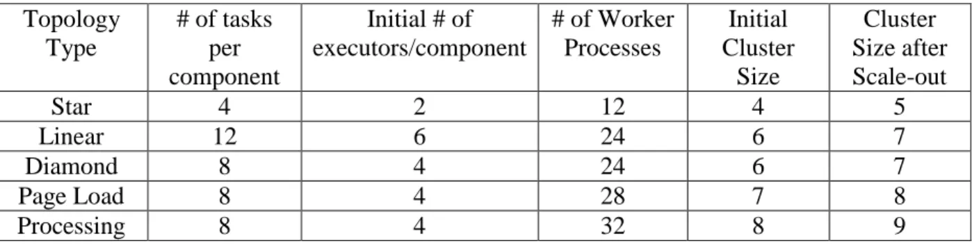
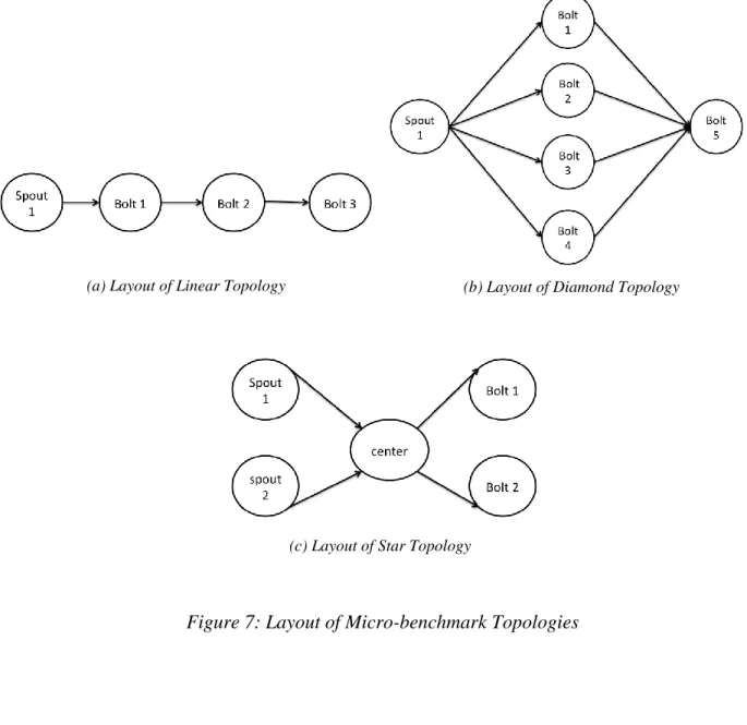
6.2.3 Micro-benchmark Storm Topologies: Linear, Diamond, and Star ... 61
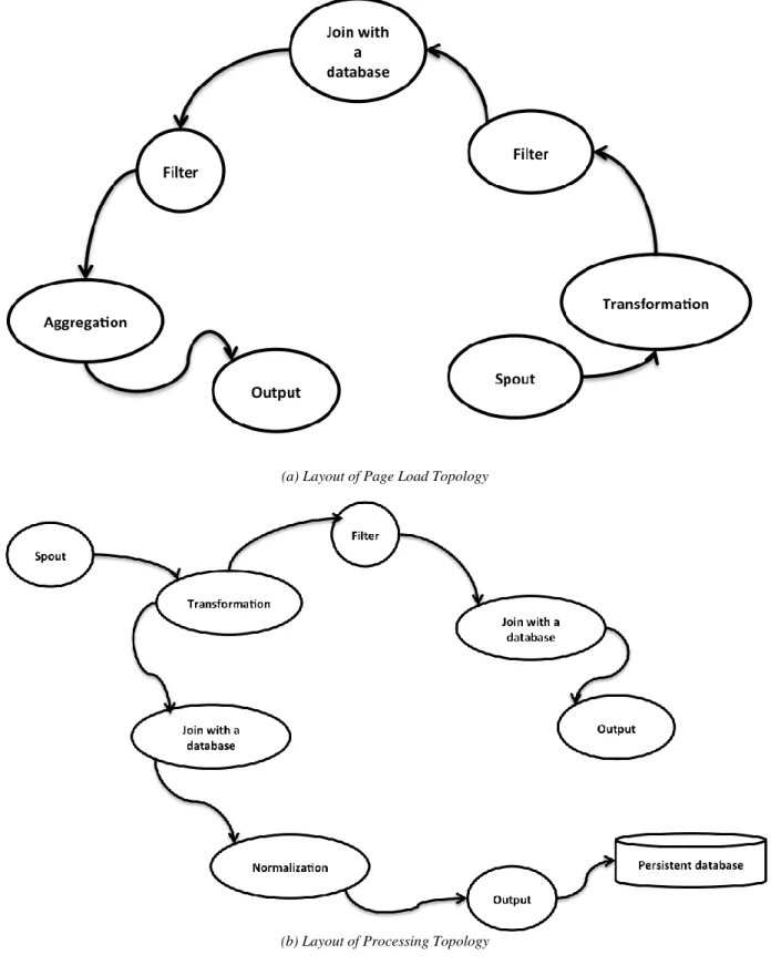
6.2.4 Yahoo Topologies: Page Load and Processing Topology ... 64
CHAPTER 7: CONCLUSION ... 67
7.1 Future Work ... 68
1
CHAPTER 1: INTRODUCTION
As our society enters an age dominated by data, processing large amounts of data in a timely fashion has become a major challenge. According to a recent article by BBC News [2], 2.5 exabytes or 2.5 billion gigabytes of data is generated every day in 2012. Seventy five percent of this is unstructured and comes for sources such as voice, text, and video. The volume of data is projected to grow rapidly over the next few years with the continued penetration of new devices such as smartphones, tablets, virtual reality sets, wearable devices, etc.
In the past decade, distributed computation systems such as [3] [4] [5] [6] [7] have been widely used and deployed to handle big data. Many systems, like Hadoop, have a batch processing model which is intended to process static data. However, a demand has arisen for frameworks that allow for processing of live streaming data and answering queries quickly. Users want a framework that can process large dynamic streams of data on the fly and serve results to potential customers with low latency. For instance, Yahoo! Needs to use a stream processing engine to perform for its advertisement pipeline processing, so that da campaigns can be monitored in real-time.
To meet this demand, several new stream processing engines have been developed recently, and are in use widely in industry, e.g., Storm [8], System S [9], Spark Streaming [10], and others [11] [12] [13]. Apache Storm is the most popular among these, and it uses a directed graph of operators (called “bolts”) running user-defined code to process the streaming data.
Unfortunately, these new stream processing systems used in industry lack many desired features. One feature is the ability to seamlessly and efficiently scale the number of servers in an
2
on-demand manner, i.e., when the user requests to increase or decrease the number of servers in the application. For instance, Storm simply un-assigns all processing operators and then reassigns them in a round robin fashion to the new set of machines. This simplistic round robin approach fails to analyze which part of the application job really needs more computation resources. Without deeper analysis into the application itself, the full benefit of adding new machines may not be reaped. Furthermore, the round robin approach could cause interruptions to ongoing computation for long durations due to potentially having reschedule every operator, which results in sub-optimal throughput after the scaling is completed.
Another feature, is an intelligent scheduler that schedules applications effectively. The current scheduler in Storm simply does a round robin scheduling of operators in the set of machines in the cluster. Such a naïve scheduling may cause resources to be not used in an efficient manner. Each application many have different resource requirement and a cluster many have different resource availabilities at the different times. By not considering resource location (in terms of network distance), resource demand, and resource availability, a scheduling may be very inefficient.
1.1
Technical Contributions
This work makes the following technical contributions:
1) We developed a System called Stela, which is, to the best of our knowledge, the first system that can create elasticity within Storm.
3
2) We provide an evaluation of Stela on a range of micro-benchmarks as well as on applications used in industry.
3) We have created a system call R-Storm that greatly improves the overall performance of Storm by scheduling applications based on resource requirement and availability.
4) We also evaluate the performance of R-Storm on a range of micro-benchmarks as well as applications used in industry.
The rest of the work is organized as follows. In Chapter 2, we provide a background on data stream processing and an overview on Storm. In Chapter 3, we introduce Storm elasticity and the system called we developed called Stela that enables efficient scale-in and -out operations in Storm. We present in detail the metrics and algorithms that went into the design of Stela. We also provide a discussion of works related to elasticity in data stream processing systems. In Chapter 4, we present a resource aware scheduler for Storm called R-Storm. We describe in detail the importance of resource aware scheduling, the problem definition, and the scheduling algorithms used in R-Storm. We also discuss works related to resource aware scheduling in the context of data stream processing systems. In Chapter 5, we provide and evaluation for both Stela and R-Storm. In Chapter 6, we provide concluding remarks.
4
CHAPTER 2: BACKGROUND
In this chapter, we first define the data stream processing model we are assuming for this paper. The data stream model we define also defines the format or data flow model of
applications running on a distributed data stream processing system. Later in the chapter, we will give a brief overview of the popular distributed data stream processing system, Storm, since this is the system our implementation targets
2.1 Data Stream Processing Model
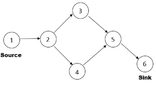
In this paper, we target distributed data stream processing systems that use a directed acyclic graph (DAG) of operators to perform the stream processing. A visual example of the above defined model is shown in Figure 1. Operators that have no parents are sources of data injection, e.g., they may read from a crawler. Operators with no children are sinks. Each sink outputs data (e.g., to a GUI or database), and the application throughput is calculated as the sum of throughputs of all sinks in the application. An application may have multiple sources and sinks.
5
Figure 1: Data Stream Processing Model
Definition 1. A data stream processing model can be referenced as a directed graph G = (V,E), where:
1. V is a set of vertices
2. E is a set of directed edges each of which is a ordered pair of vertices since G is a directed graph
3. ∀e ∈ E signifies a flow of data that can also be represented as ordered pair (vi , vj | vi
∈ V and vj ∈ V) or the pair of vertices that are connected by e
4. ∀v ∈ V represents a processing operator of a flow of data e ∈ E
5. There is a least one v ∈ V such that v is a source of information and v does not have
any parents. We call this a Source.
6. For any vi ∈ V and vj ∈ V, if there is a path vi →vj then there cannot be a path vj → vi and
vice versa. We are assuming a acyclic graph.
2.2 Overview of Storm
Storm Application: Apache Storm is a distributed real time processing framework that can process incoming live data in real time [8]. In Storm, a programmer codes an application as a Storm topology, which is a graph, typically a DAG of, operators (also referred to as components),
6
sources (called spouts), and sinks. While Storm topologies allow cycles, they are rare and we do not consider them in this paper. The operators in Storm are called bolts. Sources and sinks are also operators since they can manipulate and process data as well. The streams of data that flow between two adjacent bolts are composed of tuples. A Storm task is an instantiation of a spout or bolt - users can specify a parallelismhint to say how many tasks a bolt should be parallelized into. Storm uses worker processes, which contain executors, each of which is a thread that is spawned in a worker process that may execute one or more tasks.
The basic Storm operator, namely the bolt, consumes input streams from its parent spouts and bolts, performs processing on received data, and emits new streams to be received and processed downstream. Bolts can filter tuples, perform aggregations, carry out joins, query databases, and in general any user defined functions. Multiple bolts can work together to compute complex stream transformations that may require multiple steps, like computing a stream of trending topics in tweets from Twitter [8] Bolts in Storm are stateless. Vertices 2-6 in Figure 1 are examples of Bolts.
Storm Infrastructure: A Storm Cluster has two types of nodes: the master node, and multiple workers. The master node is responsible for scheduling tasks among worker nodes. The master node runs a daemon called Nimbus. Nimbus communicates and coordinates with Zookeeper [14] to maintain a consistent list of active worker nodes and to detect failure in the membership.
Each server runs a worker node, which in turn runs a daemon called the supervisor. The supervisor continually listens for the master node to assign it tasks to execute. Each worker contains many worker processes which are the actual containers for tasks to be executed. Nimbus
7
can assign any task to any worker process on a worker node. Multiple worker processes at a node can thus be used for multiplexing.
Each operator (bolt) in a Storm topology can be parallelized to potentially improve throughput. The user needs the explicitly specify a parallelization hint for each bolt, and Storm creates that many tasks for that bolt. Each of these concurrent tasks contains the same processing logic but may be executed at different physical locations and receive data from different sources. Data incoming to that bolt may be split among constituent tasks using one of many grouping strategies, e.g., shuffle grouping, fields grouping, all grouping, etc.
8
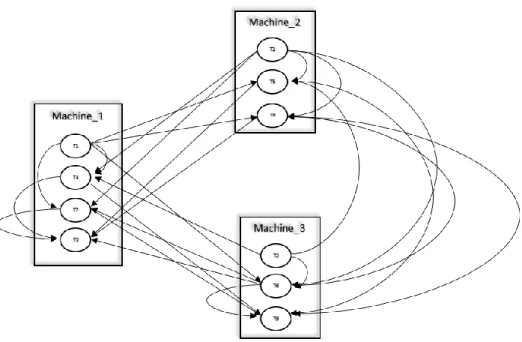
Figure 3: Actual mapping of tasks to physical machines
Storm Scheduler: Storm's default Storm scheduler (inside Nimbus) places tasks of all bolts and spouts on worker processes. Storm prefers a round robin allocation in order to balance out load, however, this may result in tasks of one bolt being placed at different workers. The default scheduler does a round robin allocation among all the worker processes on every node in the cluster. Figure 2 shows the intercommunication of tasks organized by bolt. However the actual intercommunication relative to the physical network and machines can be quite different – Figure 3 shows an example of a Storm cluster of three machines running the topology shown in Figure 2. In Figure 3 tasks are scheduled in a round robin fashion across all available machines.
9
A paper from Stanford outlined some important uses of data stream processing systems. The need for processing continuous data streams can be found in fields such as web applications, finance, security, networking, and sensor monitoring [15]. The following is a short list of real life examples
TraderBots [16] is a web-based financial service that allows uses to query live streams of financial data such as stock tickers and news feeds.
Modern security applications such as, iPolicy Networks [17], use data stream processing to inspect live packets to detect intrusion in real-time.
Yahoo [18] uses data stream processing systems to conduct real-time performance monitoring by processing large web logs produced by clickstreams to track webpages that encounter heavy traffic [19].
Several sensor monitor applications [20] [21] use data stream processing to combine, monitor, and analyze streams of data produced by sensors that distributed in the real world.
There are many other use cases for data stream applications. For a list of companies that use Apache Storm please see [8].
10
CHAPTER 3: RELATED WORK
This chapter presents a discussion of related works pertaining to elasticity in distributed systems and resource aware scheduling. We provide a list and discussion of influential works in these two areas. We also provide a discussion of how our work differentiates from other works done in these areas.
3.1
Elasticity in Distributed Data Stream Processing Systems
Stormy [11] is a distributed stream processing service recently developed by researchers for ETH Zurich and University of California, Berkeley. According the paper they published, Stormy was designed with multi-tenancy, scalability and elasticity in mind. The Stormy processing paradigm consists of queries and streams. Queries processes the data in a stream or multiple streams. Stormy organizes physical nodes into a logical ring and a node is responsible for the key space between its own and its predecessor. The technique Stormy uses for scaling in and scaling out is called Cloud Bursting. In Cloud Bursting, one node, which is elected through a leader election algorithm, determines whether to add a new node into the system or remove a node in the system. This node that determines the elastic state of the cluster is called the cloud bursting leader. If the cloud bursting leader determines that the overall load of the system is getting too high, it will introduce a new node into system. This new load will take over parts of the data range from its neighbors. The cloud bursting is a quite simple technique that might not deliver the optimal benefit of introducing new nodes into the system. When a new node in added to the system, its takes a random position on the logical ring and takes over portions of the data range of its
11
neighbors. This technique does not explore the reason why the system might be overloaded or where the primary cause of overload/bottleneck may be. In Stela, we take into account these factors when conducting elasticity operations in Storm.
Increasing the parallelism of processing operators to increase performance is not a new concept. There has been a couple papers [22] [23] from researcher at IBM T.J. Watson research that experiment with IBM System S [12] [24] [9] and SPADE [25] by increasing the parallelism of processing operators. These papers explores how increasing the parallelism of processing operators will increase performance and how to identify when peak performance of an operator is achieved. The techniques used in these papers involve applying networking concepts such as congestion control to expand and contract the parallelism of a processing operator by constantly monitoring the throughput of its links. The work of these researchers’ contrasts with our work since Stela will apply novel analytics to the processing graph as well as monitor link performance. In our work we realize that there is only a limited amount of resources to scale out to and our system intelligently identifies which processing operators, when further parallelized, will cause the overall throughput to increase the most.
Based on its predecessor Aurora [26], Borealis [27]is a stream processing engine that enables queries to be modified on the fly. Different from Stela, Borealis focuses on load balancing on a node bases and distributed load shedding in a static environment. Borealis uses correlation based operator distribution to maximize the correlation between all pairs of operators within the workflow. Borealis also uses ROD (resilient operator distribution) to determine the best operator distribution plan that is closest to an "ideal" feasible set: a maximum set of nodes that are un-overloaded.
12
StreamCloud [28] is a data streaming system designed to be elastic and scalable. StreamCloud is built on top Borealis Stream Processing Engine [13] aimed to create elasticity in the existing Borealis system. StreamCloud modifies parallelism by splitting queries into sub queries to be executed on nodes and creates a rebalancing mechanism that allows for adjustments in resources to be used. The rebalancing mechanism in StreamCloud that allows Borealis to be elastic monitors the cluster for CPU utilization. From this these statistics gathered from the cluster, StreamCloud will migrate queries or increase the parallelism of queries. StreamCloud lacks the analytics of processing graph that Stela has. Stela not only looks at resource utilization of resources in the cluster but also intelligently analyzes the processing graph to maximize the throughput of the running computation with limited amount of new resources.
3.2
Resource Aware Scheduling
Some research work has been done in the space of scheduling for Hadoop MapReduce which share many similarities with real-time processing distributed system. In the work from Jorda
et al [29], a resource-aware adaptive scheduling for a MapReduce Cluster is proposed and implemented. Their work is built upon the observation that there can be different workload jobs, and multi-users running at the same time on a cluster. By taking into account the memory and CPU capacities for each Task Tracker, the algorithm is able to find a job placement that maximizes a utility function while satisfying resource limits constraints. The algorithm is derived from a heuristic optimization algorithm to Class-Constrained Multiple Knapsack Problem which is NP-hard. However, their work fails to take network into resource constraints which is a major bottleneck for large distributed systems such as Storm.
13
Aniello et al in their paper [30] propose two scheduling algorithms for Storm. The default scheduling algorithm currently being applied in Storm does not look into the priority and the loads requirements of tasks, and simply uses a round-robin approach. As an attempt to enhance it, the authors propose a coarse version of scheduler as an offline algorithm, and later introduce an online algorithm. However, their scheduler only takes into account the CPU usage of the nodes, with an average of 20-30 percentage improvement in performance in total.
In the paper [31], Joel et al described a scheduler for System S, which is similar to Storm, a distributed stream processing system. The proposed algorithm is broken into four phases and runs periodically. At first and second phases, the algorithm decides which job to admit, which job to reject, and compute the candidate processing nodes. In the third and last phases, it computes the fractional allocations of the Processing elements to nodes. However, the approach only accounts processing power as resource and the algorithm itself is relatively complex requiring certain amount of computation.
The resource-aware scheduling in Storm needs to schedule a number of tasks into different nodes to maximize the throughput of applications (topologies) while still fulfilling the resource constrains (e.g. memory, CPU usage and bandwidth). A similar problem domain is the course timetabling problem, where we want to assign a number of events (courses) to a number of resource (classrooms) within a period of time (e.g. a week) in a way that a number of hard and soft constrains are satisfied. The goal of algorithm is to schedule tasks so that the solution satisfies given hard constraints rigidly while fulfilling soft constraints to the possible extent. The main similarity between Storm scheduling and timetabling is the fact that resource constrains in R-Storm can are also modeled as hard and soft constrains. In order to generate best throughput, it is ideal to put two tasks as close as possible if one task consumes the tuples emitted by the other task
14
(soft-constrains) as long as adding this specific task on this node will not exceed the capacity of soft and hard constrains. [32], [33], and [34] defined several variations of timetabling problems with corresponding heuristic algorithms described.
15
CHAPTER 4: STORM ELASTICITY
In this chapter, we discusses how to create elasticity in distributed data stream processing systems like Storm. We introduce a system called Stela that provide techniques for scaling in and out in distributed data stream systems. We discuss the important metrics and algorithms that went into the design of Stela. We described proposed policies for scaling-in and -out that are used in Stela.
4.1
Importance of Elasticity
Scaling-in and -out are critical tools for customers. For instance, a user might start running a stream processing application with a given number of servers, but if the incoming data rate rises or if there is a need increase the processing throughput, an administrator may wish to add a few more servers (scale-out) to the stream processing application. On the other hand, if the application is currently under-utilizing servers, then the user many want to remove some servers (scale-in) to reduce operational costs (e.g. if servers are VMs rented on AWS). Elasticity also enables users to take advantage of the pay-as-you-go model that money cloud providers adopt. Server utilization in datacenters in the real world have been estimated to be in the range from 5% to 20% [35] [36]. Thus, elasticity can majorly reduce resource waste and therefore operational cost. A more detailed analysis of cost savings when using elastic systems are explain in [37].
16
4.2
Goals
To support on-demand scaling operations, two goals are important: 1) the interruption to the ongoing computation (while the scaling operation is being carried out) should be minimized, and 2) the post-scaling throughput should be optimized. We present a system, named Stela that meets these two goals. For scale-out, Stela does this in two ways: first, it carefully selects which operators are given more resources, and secondly performs the scale-out operation in a way that is minimally obtrusive to the ongoing stream processing to the ongoing stream processing.
To select the best operators to give more resources, we need to develop metrics that can successfully capture those components (e.g., bolts and spouts in Storm) that are: i) congested and are being overburdened with incoming tuples, and ii) affect throughput the most because they have a large number of sink operators reachable from them, and iii) have many uncongested paths to their sink operators.
4.3
Stela Policy and Metrics
In this section, we focus on the scale-out operation. When the user requests a scale-out, Stela needs to decide which operators (i.e., bolts or spouts in Storm) to give more resources to (i.e., assign more tasks to). Stela first captures those operators that are congested based on their input and output rates. For it to decide the parallelization level for a congested operator, Stela needs to be able to calculate a metric for each operator that captures the percentage of total application throughput (across all sinks) that the operator has direct impact on, but by ignoring paths in the
17
DAG that are already congested. A higher value of this calculated metric needs to indicate higher performance of an operator and less likelihood that the operator contribution to the overall throughput is bounded by some congested downstream operator. This ensures that giving more resources to that operator will maximize the effect on the throughput. Given the calculated values of such a metric for each operator , Stela can iteratively assigns one or more tasks to the operator (from among those congested) that has the highest calculated value for this metric, and re-calculates a interpolated value for this metric for the future (given the latest scale-out), and iterates this process. The total number of new tasks assigned (number of iterations in Stela) ensures that the average per-server load remain the same pre- and post-scaling.
4.3.1 Determining Available Executor Slots and Load Balancing
Storm’s default scheduler distributes executors evenly across the worker nodes to guarantee each worker node is assigned a more or less equal number of executors. To retain Storm’s efficiency on a scaling operation, Stela allocates executor slots on the new worker nodes(s) such that the average number of executor slots per worker node remains unchanged. Concretely we determine the executor slots Nslots = NoriginalExecutors / MOriginal where NoriginalExecutors is the total number of executor before scaling and MOriginalis the number of worker nodes in the original cluster
18
The primary goal of Stela is to re-parallelize heavily congested operators. We consider an operator is congested when the rate of tuples an operator receives exceeds the rate of tuples it is executing. We use the procedure show in Algorithm 1 to detect have heavily congested operators. To compute the receiving rate of operator o, Stela records the number of tuples being emitted by each parent of o every 10 seconds. The input rate of operator o is calculated by averaging the sum of execution rate of all o's parents over a window of the last 200 seconds. The execution rate of o
is also calculated over the same window of time.
Algorithm 1 Detecting heavily congested operators in the topology
1: Procedure
C
ONGESTIOND
ETECTION 2: for each Operator o∈Topology do3: TotalInput ←∑ 𝐸𝑥𝑒𝑐𝑢𝑡𝑒𝑅𝑎𝑡𝑒𝑀𝑎𝑝(𝑜. 𝑝𝑎𝑟𝑒𝑛𝑡); 4: TotalOutput← ExecuteRateMap(o);
5: ifTotalInput / TotalOuput > CongestionRate then
6: add o→CongestedMap;
7: end if
8: end for return CongestedMap
9: end procedure
In Algorithm 1, when the ratio of input to output rates exceeds a threshold CongestionRate, we consider that operator to be congested. When congestion doesn't exist in an operator, the operator's receiving rate equals to execution rate. CongestionRate can be tuned as needed and it controls the sensitivity of the algorithm: lower CongestionRate values result in fewer congested operators being captured. For Stela experiments, we set CongestionRate to be 1.2. To compensate for inaccuracies in measurements, we recommend CongestionRate to be greater than 1.
19 4.3.3 Stela Metrics
Once the set of congested operators, CongestedMap, has been calculated, Stela needs to prioritize them in order to perform allocation at the limited number of extra slots (at the new worker nodes). Thus, Stela needs to utilize some sort of metric to sort these congested operators by.
There has been existing work done on metric design to capture congestion and measure throughput in data stream processing systems. An existing work [28] proposed the use of metrics such as the congestion index and throughput. The congestion index is a measure of the fraction of time a tuple is blocked due to back pressure and the throughput is the number of tuples processed over a sample period. However, these metrics do not point to the operator(s) that cause the congestion nor does it accurately suggests which operator, when further parallelized, will be likely improve the performance of the whole application. Using these one dimensional metrics also increases the time the system will need to converge when scaling-in or scaling-out since these metrics are calculated in a feedback loop that adjusts parallelism based on current results.
We decided to use the metric, Effective Throughput Percentage (ETP) [1] that more accurately captures location of congestion and the best potential operators to adjust parallelism. Below we will briefly explain how ETP of an operator is calculated.
𝐸𝑇𝑃𝑜= 𝑇ℎ𝑟𝑜𝑢𝑔ℎ𝑝𝑢𝑡𝐸𝑓𝑓𝑒𝑐𝑡𝑖𝑣𝑒𝑅𝑒𝑎𝑐ℎ𝑎𝑏𝑙𝑒𝑆𝑖𝑛𝑘𝑠
20
Here, ThroughputEffectiveReachableSinks denotes the sum of throughput of all sinks reachable from o by an un-congested path, and ThroughputWorkflow denotes the sum of throughput of all sinks of the entire workflow. The algorithm is shown in Algorithm 2.
Algorithm 2 Find Metric ETP of an operator
1: Procedure
F
INDETP
2: if o.child = null then return o.throughput; // o is a sink 3: end if
4: SubtreeeSum ← 0;
5: for each child child ∈ o do
6: if child.congested = true then
7: continue; //if the child is congested, give up the subtree rooted form the child
8: else
9: SubtreeSum = SubtreeSum +
F
INDETP
(child)
10: end if
11: end for 12:end procedure
This approach is based on two key intuitions. First, this approach prioritizes those operators that are guaranteed to effect the highest volume of sink throughput – giving more resources to this operator will certainly increase throughput of all sinks reachable via non-congested paths, because the scaling is not reducing the resources assigned to any existing operator. Second, if a congested operator has many congested paths to its reachable sinks (and thus a low ETP), assigning it more resources would have only increased the level of congestion on the downstream congested operators, which is undesirable.
21
To make the second intuition more concrete, consider two congested operators a and b, where the latter is a descendant of the former in the application DAG. Consider the set of operators
S that are b's descendants – increasing the execution rate of operator a will not improve throughput of operators in S without resolving b's congestion first. Thus the throughput produced by any operator in S will not be included while calculating ETP of a. If on the other hand operator a has no congested descendants, its ETP will be the sum of all throughput of all sinks reachable from it. Effective Throughput Percentage (ETP) is discussed in more detail in another work on elasticity [1].
4.3.4 Stela: Scale-out
During an iteration, when Stela has calculated the ETP for all congested operators, it targets the operator with the highest ETP and assigns it one extra executor slot on the newly added worker node. If multiple worker nodes are being added, then a random worker node’s executor is chosen. This algorithm runs Nslots iterations to select Nslots target operators (Section 3.3.1).
22 Algorithm 3 Stela: Scale-out
13:Procedure
S
CALE—O
UT 14: slot ← 015: while slot < 𝑁𝑠𝑙𝑜𝑡𝑠 do
16: CongestedMap ←
C
ONGESTIOND
ETECTION 17: If congestedMap.empty = true then return source18: end if
19: for each operator o∈workflow do 20: if child.congested = true then
21: ETPMap ←
F
INDETP
(Operator o)22: end if
23: end for
24: target = ETPMap.top
25: ExecutedRateMap.update(target)
26: slot ++
27: end while 28: end procedure
Algorithm 3 depicts the pseudo code. In each iteration, Stela runs Algorithm 1 to construct a CongestedMap, as explained earlier in Section 3.3.2. If the there are no congested operators in the application, Stela chooses a source operator (e.g., a Spout in Storm) as a target to increase the input rate of the entire workflow – this increases the rate of incoming tuples to the entire application. If congested operators do exist, for each operator, Stela finds its ETP using the algorithm discussed in Section 3.3.3. The result is sorted into ETPMap. Stela chooses the operator that has the highest ETP value from ETPMap as a target for the current iteration. It assigns this operator an extra slot on one of the new workers nodes.
For the next iteration, Stela estimates the execution rate of the target operator proportionally, i.e., if the operator previously had an execution rate E and k tasks, then its new
23
projected execution rate is 𝐸(𝑘+1
𝑘 ). This is a reasonable approach since all workers have the same number of tasks and thus proportionality holds.
Now Stela once again calculates the ETP of all operators in the application -- we call these ETP values as projected ETP, because they are based on estimates. These iterations are repeated until all available executor sets are filled.
In Algorithm 3, procedure FindETP involves searching for all reachable sinks for every congested operator -- as a result each iteration of Stela has a running time complexity of O(n2)
where n is the number of operators in the workflow. The entire algorithm has a running time complexity of O(m n2), where m is the number of new executor slots at the new worker node(s).
4.3.5 Stela: Scale-in
The techniques used in scale-out can also be used for scale-in, most importantly, the ETP metric. However, for scale-in we will not be calculating the ETP per operator but per machine in the cluster. For scale-in, we first, calculate the ETPSum for each machine. ETPSum is defined as:
𝐸𝑇𝑃𝑆𝑢𝑚(𝑚𝑎𝑐ℎ𝑖𝑛𝑒𝑘) = ∑ 𝐹𝑖𝑛𝑑𝐸𝑇𝑃)𝐹𝑖𝑛𝑑𝐶𝑜𝑚𝑝(𝜏𝑖))
𝑛
𝑖=1
ETPSum for a machine is the sum of all ETP of instances of operators that reside of the machine. Thus, for every task, 𝜏𝑖, that resides on machine, 𝜏𝑖, we first find the operator 𝜏𝑖 is an instance of and then find the ETP of that operator. After, to get ETPSum, we sum all the ETPs.
24
ETPSum of a machine is an indication of how much the tasks executing on that machine contribute to the overall throughput. Therefore, in general, ETPSum can be thought of as an importance metric of a machine. The intuition behind ETPSum is that a machine with lower ETPSum is better candidate to be removed in a scale-in operation than a machine with higher ETPSum since a machine with lower ETPSum negatively influence the application less in both throughput and downtime to the running application.
Algorithm 4 Stela: Scale-In
1: Procedure
S
CALE—I
N2: for each Machine 𝑛 ∈ 𝑐𝑙𝑢𝑠𝑡𝑒𝑟 do
3: 𝐸𝑇𝑃𝑀𝑎𝑐ℎ𝑖𝑛𝑒𝑀𝑎𝑝 ← ETP
M
ACHINES
UM(n)4: end for
5: 𝐸𝑇𝑃𝑀𝑎𝑐ℎ𝑖𝑛𝑒𝑀𝑎𝑝. 𝑠𝑜𝑟𝑡() // sort ETPSum in increasing
order
6:
R
EMOVEM
ACHINE(𝐸𝑇𝑃𝑀𝑎𝑐ℎ𝑖𝑛𝑒𝑀𝑎𝑝. 𝑓𝑖𝑟𝑠𝑡()) 7: end procedure8: Procedure
R
EMOVEM
ACHINE(Machine n, ETPMa-chineMap map)9: for each task 𝜏𝑖 on Machine n do 10: if i > map.size then 11: 𝑖 ← 0 12: end if 13: Machine 𝑥 ← 𝑚𝑎𝑝. 𝑔𝑒𝑡(𝑖) 14: ASSIGN(𝜏𝑖, 𝑥) 15: 𝑖 + + 16: end for 17:end procedure
When a scale-in operation needs to occur, the SCALE-IN procedure in Algorithm 4 is called. The procedure calculates the ETPSum for each machine in the cluster and puts the machine
25
and its corresponding ETPSum in the ETPMachineMap. The ETPMachineMap is sorted by ETPSum values in increasing order. The machine with the lowest ETPSum will be the target machine to be removed in this round of scale-in. We then call the procedure RemoveMachine to reschedule the tasks of the machine with the lowest ETPSum.
Tasks from the machine that is chosen to be removed are re-assigned to the other machines in the cluster in an iterative manner. Tasks will first be assigned one at a time starting with machines with lower ETPSum. Since there is an expectation that existing tasks running on a machine will be negatively affected by the addition of new tasks, this heuristic dampens the overall negative effect of assigning additional tasks to machines.
The intuition is that task additions to machines with lower ETPSum will have less of an effect on the overall performance since machines with less ETPSum contributes less to the overall performance. Starting the assignment of tasks to be rescheduled on machines with lower ETPSum will not only dampen the potential decrease in overall performance but also help shorten the amount of downtime the application will experience due to the rescheduling. When adding new tasks to a machine, existing tasks may need to be paused for a certain duration. Tasks on a machine with lower ETPSum contributes less to the overall performance and thus causes less overall downtime for the application.
4.4
Implementation
We have implemented Stella as a custom scheduler inside Apache Storm. A user may create a custom scheduler by creating a Java class that implements a predefined IScheduler
26
interface. The scheduler runs as part of the Storm Nimbus daemon. A user specifies which scheduler to use in a YAML formatted configuration file call storm.yaml. If no scheduler is explicitly specified, Storm will use its default scheduler for scheduling. The Storm scheduler is invoked by Nimbus periodically, with a default time period set to 10 seconds. Storm Nimbus is a stateless entity and thus, the Storm scheduler cannot store information across multiple invocations.
4.4.1 Core Architecture
Figure 4: Implementation Diagram
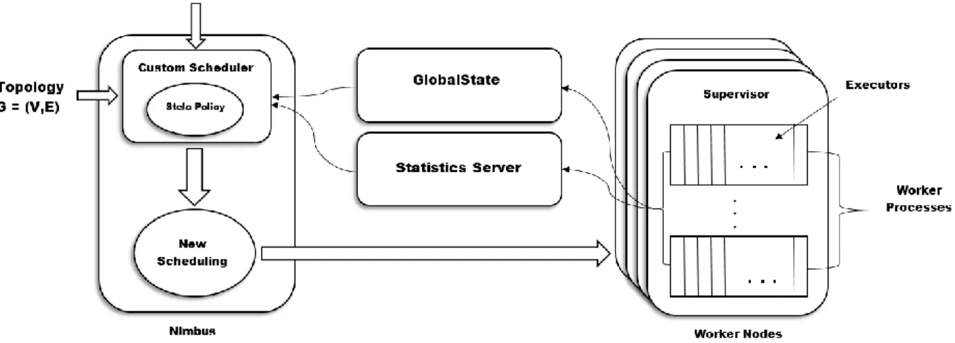
The architecture of the implementation in Storm is visually presented in Figure 5. Our implementation of Stela in Storm consists of three modules:
StatisticServer - This module is responsible for collecting statistics in the Storm cluster, e.g., throughput at each task, bolt, and for the topology. This data is used as input to Algorithm 1 and 2 in Section 3.3.2 and 3.3.3, respectively.
27
GlobalState - This module stores important state information regarding the scheduling and performance of a Storm Cluster. This module holds information about where each task is placed in the cluster. This module also stores statistics like sampled throughputs of incoming and outgoing traffic for each bolt for a specific duration used to determine congested operators as mentioned in section 3.3.2 and serves as one of the inputs for Algorithm 1.
Strategy - This module provides an interface for scale-out strategies to implement so that strategies can be easily swapped in and out for evaluation purposes. This module calculates a new schedule based on the scale-out strategy in use and may use information from the Statistics and GlobalState modules. The core Stela policy (Section 3.3.4) and Topology Aware strategies (Section 3.4.2) are implemented as a part of this module.
ElasticityScheduler - This module is the custom scheduler that implements IScheduler interface. This class starts and initializes the StatisticServer and
GlobalState modules. It also invokes the Strategy module to calculate a new scheduling when the scale-out needs to take place.
When a scale-in or -out signal is sent to the ElasticityScheduler, a procedure is invoked that detects newly joined machines based on previous membership. If no new machines are detected, the scale-in or -out procedure aborts. If new machines are found, the ElasticityScheduler invokes the Strategy module, which calculates the new scheduling. The new scheduling is then returned to the ElasticityScheduler and ElasticityScheduler will modify the current scheduling in the cluster accordingly.
28 4.4.2 Topology Aware Strategies
Initially, before we settled on the Stela design in Section 3.3, we attempted to design several topology-aware strategies for scaling out. We describe these below, and we will compare the approach based on Metrix X against these in our experiments in Section 3.5. They are thus a point of comparison for Stela.
Topology-aware strategies migrate existing tasks instead of increasing the parallelism of tasks as Stela does. These strategies aim to find “important” components/processing operators in a Storm Topology. These components that are deemed “important” are given priority to use additional resources when new nodes join the membership. We list some of the topology-aware strategies we developed.
Distance from spout(s) - In this strategy, we prioritize components that are closer to the source of information as defined in Section 2.1. The rationale for this method is that if a component that is more upstream is a bottleneck, it will affect the performance of all bolts that are further downstream.
Distance to output bolt(s) - In this strategy, higher priority for use of new resources are given to bolts that are closer to the sink or output bolt. The logic here is that bolts right connected near the sink affect the throughput the most.
Number of descendants - In this strategy, importance is given to bolts with many descendants (children, children's children, and so on) because bolts with more descendants potentially have a larger effect on the overall application throughput.
29
Centrality - In this strategy, higher priority is given to bolts that have a higher number of in- and out-edges adjacent to them (summed up). The intuition is that “well-connected” bolts have a bigger impact on the performance of the system then less well-connected bolts.
Link Load - In this strategy, higher priority is given to bolts based on the load of incoming and outgoing traffic. This strategy examines the load of links between bolts and migrates bolts based on the status of the load on those links. Similar strategies have been used in [30] to improve Storm's performance. We have implemented two strategies for evaluation: Least Link Load and Most Link Load. Least Link Load strategy sorts executors by the load of the links it’s connected to and starts migrating tasks to new workers in by attempting to maximize the number of adjacent bolts that are on the same server. The Most Link Load strategy does the reverse.
During our measurements, we found that the Least Link Load based strategy is the most effective in improving performance among all the strategies mentioned above. Thus the Least Link Load based strategy is representative of strategies that attempt to minimize the network flow volume in the topology schedule. Hence in the next section, we will compare the performance of the Least Link Load based strategy with Stela.
30
CHAPTER 5: RESOURCE AWARE SCHEDULING IN STORM
In this chapter, we provided a detail description of resource aware scheduling in Storm. We introduce a system called R-Storm that schedules applications with considerations to resource requirements and resource availability in the underlying cluster. We introduce the notion of soft and hard resource constraints. We will discuss in detail the policies and algorithms used in R-Storm to schedule tasks within a topology such that violations to soft constraints are minimized and violations to hard constraints are prevented. To find an optimal scheduling, the problem can be mapped to a Quadratic Multiple 3-Dimensional Knapsack Problem of class NP-Hard. However, our proposed scheduling algorithm within R-Storm circumvents these
computational challenges by using heuristics.
5.1
Importance of Resource Aware Scheduling in Storm
The importance of creating a new and intelligent scheduler in Storm is due to the naïve and over simplistic scheduler that is in current use within Storm. The current default scheduler within Storm simply applies a round robin scheduling of all executors of a topology to nodes in the cluster. Storm’s default scheduler does neither take into account the resource requirements of the topology that the user wishes to run or the resource availability of the cluster that Storm is executing in.
A Storm topology is a user-defined application that can have any number of resource constraints for it to run. Not considering resource demand and resource availability when
31
scheduling can be problematic. The resource on machines in the cluster can be easily over-utilized or under-utilized with can cause problems ranging from catastrophic failure to execution inefficiency. For example, a Storm cluster can suffer a potentially unrecoverable failure if certain executors attempt to use more memory than is available on the machine the executor resides on. Over-utilization of resource other than memory can also cause the execution of topologies to grind to a halt. Under-utilization decreases resource utilization and can cause unnecessary expenditures in operating costs of a cluster. Thus, to maximize performance and resource utilization, an intelligent scheduler must take into account resource availability in the cluster as well as resource demand from a storm topology in order to calculate an efficient scheduling.
5.2
Problem Definition
The question we are trying to answer is how to assign tasks to machines. Each task has a set of certain resource requirements and each machine in a cluster has a set of resources that are available. Given these resource requirements and resource availability how can we create a scheduling such that, for all tasks, every resource requirement is satisfied if possible? Thus, the problem becomes find a mapping of tasks on machines such that every resource requirement is satisfied and at the same time no machine is exceeding its resource availability.
In this work, we consider three different types of resources: CPU usage, memory usage, and bandwidth usage. We define CPU resources as the project CPU usage/availability percentage, memory resources as the megabytes used or available, and bandwidth as the network distance between to nodes. We classify them as two different classes: hard constraints and soft constraints.
32
Hard constraints are resources which cannot exceeded, while soft constraints relates to resources which can be exceeded. In the context of our system, CPU and bandwidth budgets are considered soft constraints as they can be overloaded, while the memory is considered as a hard constraint as we cannot exceed the total amount of available memory.
In general, the number of constraints to use and whether a constraint is soft or hard is specified by the user. The reasoning behind having hard and soft constraints is that some resources have a graceful degradation of performance while others do not. For example, the performance of computation and network resources degrade as over utilization increases. However, if a system attempts to use more memory resources than physically available the consequences are catastrophic. We have also identified that to improve performance sometimes it is beneficial to over utilize one set of constrained resources but gain better utilization of another set of soft-constrained resources. We assume that for each node of the cluster there is a specific limited budget for these resources. Similarly, each task specifies how much of each type of resource it needs. The goal is to efficiently assign tasks to different worker nodes while minimizing the total amount of resource usage. This problem can essentially be modeled as a linear programming optimization problem as we will discuss next.
Let T = (τ1, τ2 , τ3 , . . .) be the set of all tasks within a topology. Each task τi has a soft constraint CPU requirement of 𝑐𝜏𝑖𝑗 , a soft constraint bandwidth requirement of 𝑏𝜏𝑖, and a hard constraint memory requirement of 𝑚𝜏𝑖. We will discuss the notion of soft and hard constraints more in the next section. Similarly, let N = (θ1 , θ2 , θ3 , . . .) be the set of all nodes, which correspond to total available budgets of W1 , W2 , and W3 for CPU, bandwidth, and memory. For the purpose of quantitative modeling, let the throughput contribution of each node to be 𝑄𝜃𝑖. The
33
goal here is to assign tasks to a subset of nodes N’ ⊆ N that maximizes the total throughput while tasks not exceeding the budgets W1, W2, and W3. In other words,
𝑀𝑎𝑥𝑖𝑚𝑖𝑧𝑒 ∑ ∑ 𝑄𝜃𝑖𝑗 𝑗 ∈𝑛𝑜𝑑𝑒𝑠 𝑖 ∈𝑐𝑙𝑢𝑠𝑡𝑒𝑟𝑠 𝑠. 𝑡. ∑ ∑ 𝑐𝜏𝑖𝑗 𝑗 ∈𝑛𝑜𝑑𝑒𝑠 𝑖 ∈𝑐𝑙𝑢𝑠𝑡𝑒𝑟𝑠 < 𝑊1 𝑎𝑛𝑑 ∑ ∑ 𝑏𝜏𝑖𝑗 𝑗 ∈𝑛𝑜𝑑𝑒𝑠 𝑖 ∈𝑐𝑙𝑢𝑠𝑡𝑒𝑟𝑠 < 𝑊2 𝑎𝑛𝑑 ∑ ∑ 𝑚𝜏𝑖𝑗 𝑗 ∈𝑛𝑜𝑑𝑒𝑠 𝑖 ∈𝑐𝑙𝑢𝑠𝑡𝑒𝑟𝑠 < 𝑊3
Which is simplified into:
𝑀𝑎𝑥𝑖𝑚𝑖𝑧𝑒 ∑ 𝑄𝜃𝑖 𝜃 ∈𝑁′ 𝑆𝑢𝑏𝑗𝑒𝑐𝑡 𝑡𝑜 ∑ 𝑐𝜏𝑖𝑗 𝜏 ∈𝑁′ < 𝑊1 , ∑ 𝑏𝑖𝑗 𝜏 ∈𝑁′ < 𝑊2 , ∑ 𝑚𝜏𝑖𝑗 𝜏 ∈𝑁′ < 𝑊3
This selection and assignment scheme is a complex and a special variation of Knapsack optimization problem. The well-known binary Knapsack problem is NP-hard but efficient approximation algorithms can be utilized (fully polynomial approximation schemes), so an approach is computationally feasible. However, the binary version, which is the most common Knapsack problem only considers a single constraint and enables only a subset of the tasks to be
34
selected, which is not desired as we need to assign all the tasks to the nodes, considering that there are multiple constraints.
To overcome the shortcomings of the binary Knapsack approach, we need to formulate the problem as other variations of Knapsack problem, which eventually assigns all the tasks to the nodes.
The first different concept in our formulation is the fact that our problem consists of multiple knapsacks (i.e. clusters and corresponding nodes). This may seem like a trivial change, but it is not equivalent to adding to the capacity of the initial knapsack. This variation is used in many loading and scheduling problems in Operations Research [38]. Thus our problem corresponds to a Multiple Knapsack Problem (MKP), in which we assign tasks to multiple different constrained nodes.
The second insight that we need to consider in our formulation is that if there is more than one constraint for each knapsack (for example, given knapsack scenario, both a volume limit and a weight limit, where the volume and weight of each item are not related), we get the multidimensional knapsack problem, or m-Dimensional Knapsack Problem. In our problem, we need to address 3 different resources (i.e. CPU, bandwidth, and memory constraints) which leads to a 3-Dimensional Knapsack Problem.
The third concept that we need to consider is that given the topology, assigning two successive tasks on the same node is more efficient than assigning them on two different nodes, or even two different clusters. This is another special variation of knapsack problem, called Quadratic Knapsack Problem (QKP) introduced by Gallo et al. [39] [40], which consists in choosing
35
elements from n items for maximizing a quadratic profit objective function subject to a linear capacity constraint.
Our problem is a Quadratic Multiple 3-Dimensional Knapsack Problem (we call it QM3DKP). We propose a heuristic algorithm that assigns all tasks to multiple nodes while with a higher probability two successive tasks being on the same node. The heuristic algorithm needs to be simple with low overhead to be suitable for real-time requirements of Storm applications.
Different variations of knapsack problem has been applied to certain contexts. Y. Song et al in their paper [41] investigated the multiple knapsack problem and its applications in cognitive radio networks. In their paper, a centralized spectrum allocation in cognitive radio networks has been formulated as a multiple knapsack problem. Lamani et al [42] also proposed an end-to-end quality of service to tackle the problem of setting end-to-end connections across heterogeneous domains modeling the complexity as a multiple choice knapsack problem. X. Xie and J. Liu in their paper [43] studied QKP, while also in [44], the authors applied the concept of m-dimensional knapsack problem for the first time to the packet-level scheduling problem for a network, and proposed an approximation algorithm for that.
Many algorithms have been developed to solve various knapsack problems using dynamic programming [45] [46], tree search (such as A*) techniques used in AI [47] [48], approximation algorithms [49] [50], and etc. However, these algorithms are constraining in terms of computational complexity even though some algorithms have pseudo polynomial runtime complexity. Most, if not all, of these algorithms would require much more time to compute a scheduling that than necessarily available in a distributed data stream system. Since data stream systems are required to respond to events as close to real-time as possible, scheduling decisions
36
need to be made in a snappy manner. The longer the scheduling takes to compute, the longer the downtime an application will have.
5.3
Proposed Algorithm
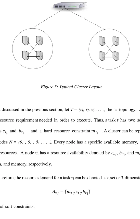
In data centers, servers are usually placed on a rack connected to each by a top of rack switch. The top of rack switch is also connect to another switch which connects server racks together. The network layout can be represented by Figure 11. Data centers with this kind of layout is likely where Storm clusters are going to be deployed. The design of our algorithm is influenced by the environment Storm is going to be run in.
1) Inter-rack communication is the slowest 2) Inter-node communication is slow 3) Inter-process communication is faster 4) Intra-process communication is the fastest
37
Figure 5: Typical Cluster Layout
As discussed in the previous section, let T = (τ1, τ2, τ3 , . . .) be a topology. A task has a set of resource requirement needed in order to execute. Thus, a task τi has two soft resource
constraints 𝑐𝜏𝑖 and 𝑏𝜏𝑖 and a hard resource constraint 𝑚𝜏𝑖 . A cluster can be represented as a set of nodes N = (θ1 , θ2 , θ3 , . . .). Every node has a specific available memory, CPU, and network resources. A node θi has a resource availability denoted by 𝑐𝜃𝑖, 𝑏𝜃𝑖, and 𝑚𝜃𝑖 for CPU,
bandwidth, and memory, respectively.
Therefore, the resource demand for a task τi can be denoted as a set or 3-dimensional vector, 𝐴𝜏𝑗 = {𝑚𝜏𝑖, 𝑐𝜏𝑖, 𝑏𝜏𝑖}
and a set of soft constraints,
38 and set of hard constraints,
𝐻𝜏𝑖 = {𝑚𝜏𝑖} Such that 𝐻𝜏𝑖 ⊆ 𝐴𝜏𝑖 𝑆𝜏𝑖 ⊆ 𝐴𝜏𝑖 and, 𝐴𝜏𝑖 = 𝑆𝜏𝑖 ∪ 𝐻𝜏𝑖
The resource availability of a node θi can be denoted as a set or 3-dimensional vector,
𝐴𝜃𝑖 = {𝑚𝜃𝑖, 𝑐𝜃𝑖, 𝑏𝜃𝑖}
and a set of soft constraints,
𝑆𝜃𝑖 = { 𝑐𝜃𝑖, 𝑏𝜃𝑖}
and set of hard constraints,
𝐻𝜃𝑖 = { 𝑚𝜃𝑖 }
Such that
𝐻𝜃𝑖 ⊆ 𝐴𝜃𝑖 𝑆𝜃𝑖 ⊆ 𝐴𝜃𝑖
39
𝐴𝜃𝑖 = 𝑆𝜃𝑖 ∪ 𝐻𝜃𝑖
We can generalize the resource demand of a specific task and the resource availability of a node as a n-dimensional vector residing in ℝ𝑛.
Each soft constraint can have a weight attached to it, such that:
|W | = |S| S0 = W · S
The reason for allowing constraints to be weighted is to enable normalized values for comparison purposes, as well as facilitating in providing more importance to more valued constraints.
5.3.1 Algorithm Description
Given a task τi , a vector 𝐴𝜏𝑖 of each task’s resource demands and a cluster N = (θ1 ,
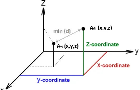
θ2 , θ3 , . . .) with each node θi and a vector 𝐴𝜃𝑖 of each node’s resource availability, the algorithm determines which node to schedule a task on. Assuming that each resource corresponds to an axis, we find the node 𝐴𝜃𝑖 that is closest in Euclidean distance to 𝐴𝜏𝑖 such that 𝐻𝜃𝑖 > 𝐻𝜏𝑖 for all hard constraints, so that no hard constraints are violated. We choose θi as the node where we schedule task τi, and then update the available resources left on 𝐴𝜃𝑖 . We continue this process until all tasks get scheduled on nodes. Algorithm 5 describes a pseudo-code of our proposed heuristic algorithm.
40 Algorithm 5 Proposed Heuristic Algorithm
1: Procedure
R
-STORM2: 𝐴𝜃: set of all nodes 𝜃𝑖 in the n-dimensional space // (n=3 in our context 3: 𝐴𝜏: set of all tasks 𝜏𝑖 in the n-dimensional space // (n=3 in our context) 4: 𝐴𝜃𝑖: n-dimensional vector of resource availability of a node 𝜃𝑖, such that
𝐴𝜃𝑖 ∈ 𝐴𝜃
5: 𝐴𝜏𝑖:n-dimensional vector of resource requirement of a task 𝜏𝑖, such that 𝐴𝜏𝑖 ∈ 𝐴𝜏
6: for each task 𝜏𝑖 do
7: select 𝐴𝜃𝑗 = min 𝑑 (𝐴𝜃𝑗, 𝐴𝜏𝑖) ∀𝐴𝜏𝑗 ∈ 𝐴_𝜏 given 𝑑(𝜆, 𝜆′) ←
√(𝜆′× 𝑥 − 𝜆 × 𝑥)2 + (𝜆′× 𝑦 − 𝜆 × 𝑦)2+ (𝜆′× 𝑧 − 𝜆 × 𝑧)2 ∀𝜆 ∈
𝐴𝜏 , 𝜆 ∈ 𝐴𝜃 and 𝐻𝜃𝑖 > 𝐻𝜏𝑖 // for all hard resource constraints 8: 𝐴𝜃𝑗 ← 𝐴𝜃𝑗− 𝐴𝜏𝑖 //update the resource vector 𝐴𝜃𝑗 of selected node
9: end for 10: end procedure
In Algorithm 5, Line 2 and 3 declares a list of nodes in the cluster and a list of tasks that need to be scheduled. Line 4 declares that for each node in the cluster there is an n-dimensional vector representing n-declared resource availabilities for that node. Similarly, Line 5 declares that for each task that needs to be scheduled an n-dimensional vector representing n-declared resource requirements for running an instance of that task. Thus, a node and task can be
represented as a point or vector in an n-dimensional space. Line 6-8 describes how the tasks are scheduled. We iterate through the list of tasks that need to be scheduled and for each task represented as a vector in an n-dimensional space, we find the node vector (represents node resource availability) that is closes in Euclidian distance to the task vector. The node vector must also reside above up to n different planes that represent hard resource constraints. Thus, the node vectors we consider are the ones that must be able to satisfy fully all the hard resource constraints of the task.
41
1) Two successive tasks given the topology are scheduled on closest nodes, which ensures the intercommunication insights as described in the previous section. 2) No hard resource constraints is violated.
3) Resource wastes on nodes are minimized
Figure 6 shows a visual example of a selected minimum-distance node to a given task in the 3D resource space, while the hard resource constraint (i.e. Z axis) is not violated. Our algorithm consists of two parts, task selection and node selection.
Figure 6: An example node selection in a 3D resource space
42
For task selection, given the topology there should be a start point as well as a traversal algorithm. We assume that our algorithm starts selecting tasks from Spouts, which is discussed in Section 2.2. However, the starting point can be user defined based on which component the user deems the most important to the topology. For example, heuristics to determine the starting point could be: 1) most well connected component. The component with most directly connected neighbors. 2) The component with most descendants. 3) Components closer to the sinks and etc. As for the traversal algorithms, we consider two popular graph traversal algorithms, breadth first search (BFS) and depth first search (DFS). Both of these construct spanning trees with certain properties useful in graph algorithms. In the BFS traversal, we just keep a tree (the BFS tree), a list of tasks to be added to the tree, and markings (Boolean variables) on the tasks to tell whether they are in the tree or list. BFS traversal of the tasks corresponds to some kind of tree traversal. But it isn't preorder, post-order, or even in-order traversal. Instead, the traversal goes a specific level at a time, left to right within a level (where a level is defined simply in terms of distance from the spout). The DFS algorithm is the other way of our task selection approach, which is closely related to preorder traversal of a tree.
To prevent infinite loops, we only want to visit each task once. Just like in BFS we use marks to keep track of the tasks that have already been visited, so not to visit them again. Our overall DFS traversal then simply initializes a set of markers, and just like in the BFS traversal, if a task has several intercommunicated neighbors it would be equally correct to go through them in any order. We'll start by the Spout, and use one of these two traversal algorithms to select next task.
Take the topology depicted in Figure 1 for example. If we were to start our task selection at the spout, component 1 would be our starting point. Then we would traverse the topology in a
43
depth first manner. Thus, the ordering of the traversal would be 1, 2, 3, 4, 5, and 6. A task is selected to be scheduled at component 1, then at component 2 and so on. Once we scheduled a task belonging to component 6 and there are still remaining tasks waiting to be scheduled for components previous in the traversal ordering, we loop back and schedule them according to the traversal ordering. We do this until every task is scheduled.
5.3.3 Node Selection
After a task is selected, a node needs to be selected to run this task. If the task that needs to be scheduled is the first task in a topology, find the server rack or sub-cluster with the most available resources. Afterwards, find the node in that server rack with the most available resources and schedule the first task on that node which we will refer to as the reference node or Ref Node. For the rest of the tasks in the Storm topology, we will find nodes to schedule based on the Algorithm 1 with our bandwidth attribute 𝑏𝜃𝑖 defined as the network distance from
Ref Node to node 𝜃𝑖 . By selecting nodes in this manner, tasks will be patched as tightly on and closely around the Ref Node as resource constraints allow, which minimizes the network latency of tasks communicating with each other.
5.4
Implementation
We have implemented R-Storm as a custom version of Storm. We have modified the core Storm code to allow physical machines to send their resource availability to Nimbus. The core