Airline fleet assignment concepts, models, and algorithms

(1)

Invited Tutorial

Airline ﬂeet assignment concepts, models, and algorithms

Hanif D. Sherali

*

_{, Ebru K. Bish, Xiaomei Zhu}

Grado Department of Industrial and Systems Engineering (0118), Virginia Polytechnic Institute and State University, Blacksburg, VA 24061, United States

Received 5 May 2004; accepted 3 January 2005 Available online 2 April 2005

Abstract

Thefleet assignment problem(FAP) deals with assigning aircraft types, each having a different capacity, to the sched-uled flights, based on equipment capabilities and availabilities, operational costs, and potential revenues. An airlineÕs fleet-ing decision highly impacts its revenues, and thus, constitutes an essential component of its overall schedulfleet-ing process. However, due to the large number of flights scheduled each day, and the dependency of the FAP on other airline processes, solving the FAP has always been a challenging task for the airlines. In this paper, we present a tutorial on the basic and enhanced models and approaches that have been developed for the FAP, including: (1) integrating the FAP with other airline decision processes such as schedule design, aircraft maintenance routing, and crew scheduling; (2) proposing solu-tion techniques that include addisolu-tional considerasolu-tions into the tradisolu-tional fleeting models, such as considering itinerary-based demand forecasts and the recapture effect, as well as investigating the effectiveness of alternative approaches such as randomized search procedures; and (3) studying dynamic fleeting mechanisms that update the initial fleeting solution as departures approach and more information on demand patterns is gathered, thus providing a more effective way to match the airlineÕs supply with demand. We also discuss future research directions in the fleet assignment arena.

Keywords: Airlines; Fleet assignment; Integer programming; Large scale optimization; Transportation

1. Introduction

Aircraft seats are an airlineÕs product. Similar to any other product, a larger quantity secures sales, while extra inventory incurs costs. For airlines, providing larger capacities implies higher operating costs. On the other hand, aircraft seats are ‘‘perishable’’, that is, unsold seats at the departure of the ﬂight are wasted. Consequently, the ideal strategy is to provide just the ‘‘right number’’ of seats to passengers at the ‘‘right

*

Corresponding author. Tel.: +1 540 231 5474; fax: +1 540 231 3322.

E-mail addresses:[email protected](H.D. Sherali),[email protected](E.K. Bish),[email protected](X. Zhu).

(2)

price’’. The ﬁrst of these two ideals is addressed by the ﬂeet assignment process, which is the subject of the present paper, while the second falls in the purview of yield or revenue management.

Thefleet assignment problem(FAP) deals with assigning aircraft types, each having a different capacity, to the scheduled flights, based on equipment capabilities and availabilities, operational costs, and potential revenues. An airlineÕs fleeting decision highly impacts their revenues: Assigning a smaller aircraft than needed on a flight will result inspilled(i.e., lost) customers due to insufficient capacity; assigning a larger aircraft will result inspoiled(i.e., unsold) seats, and presumably higher operational costs. Thus, FAP con-stitutes an essential component of an airlineÕs overall scheduling process. However, due to the large number of flights scheduled each day, which can easily reach thousands for a major airline, and the dependency of the FAP on other airline processes such as schedule design, crew scheduling, aircraft routing, maintenance planning, and revenue management, solving the FAP has always been a challenging task for the airlines. As a result, it is not surprising that the FAP has been extensively studied in the Operations Research literature. However, most of the traditional approaches proposed for the FAP depend on solving the FAP in isolation from the other airline scheduling processes and under restrictive assumptions such as considering the same-every-day schedule; and using point forecasts for flight-based demands instead of itinerary-based or path-based demands. Furthermore, customers rejected from their requested itineraries (due to capacity restrictions) are often assumed to be lost. In reality, they may choose to take another route that is compa-rable to their first choice itinerary in terms of the origin, destination, and time-frame (i.e., they may be recaptured). The recapture effect has mostly been ignored in analytical studies until very recently.

Recent advances in information technology, coupled with an increasingly competitive marketplace, have motivated researchers to consider new approaches for the FAP over the last decade. These new directions include: (1) integrating the FAP with other airline decision processes such as schedule design, aircraft main-tenance routing, and crew scheduling; (2) proposing solution techniques that include additional consider-ations into the traditional fleeting models, such as considering itinerary-based demand forecasts and the recapture effect, as well as investigating the effectiveness of alternative approaches such as randomized search procedures; and (3) studying dynamic fleeting mechanisms that update the initial fleeting solution as departures approach and more information on demand patterns is gathered, thus providing a more effec-tive way to match the airlineÕs supply with demand.

The aim of this paper is to present a tutorial on the basic and enhanced models and approaches that have been developed for the FAP as well as to suggest some future research directions in this arena. For the sake of exposition, we focus on several key recent papers on the FAP, instead of providing an exhaustive survey in this area, for which we refer the interested readers to the review articles byGopalan and Talluri (1998), Yu and Yang (1998), Barnhart et al. (2004), Clarke and Smith (2004), andKlabjan (in press). A special issue of Transportation Science (Ball, 2004) also provides a variety of topics on aviation operations research.

The remainder of this paper is organized as follows: We first introduce the terminology that will be used throughout this paper in Section 2. We then proceed to describe the various fleet assignment models (FAM) in the subsequent sections. Specifically, the basic FAM as well as the proposed solution approaches are dis-cussed in Section 3. Section 4 presents various approaches that aim at integrating the FAM with other air-line decision processes. Section 5 addresses enhanced FAMs that include certain additional considerations, and Section 6 covers some dynamic fleeting models. Finally, Section 7 concludes this paper with some rec-ommendations for future research directions in this area.

2. Terminology

Fleet type(aircraft type): A certain model of aircraft, such as BoeingÕs B767-300. All aircraft of the same type have the same cockpit conﬁguration, crew qualiﬁcation requirements, maintenance requirements, and capacity.

(3)

Fleet family (aircraft family): A set of aircraft types, each having the same cockpit configuration and crew qualification requirements. Thus, the same crew can fly any aircraft type of the same family. An exam-ple of an aircraft family is the Boeing 757/767 family, which consists of multiexam-ple aircraft types, such as the B757-200 and the B767-300, having capacity ranges between 186 and 255 passengers.

Leg(flight leg): An airport-to-airport flight segment that starts at a specific departure time and connects two stops of a flight, i.e., a leg spans the journey from the time an aircraft takes off until it lands.

Path(itinerary): A sequence of one or more flight legs between a specific origin and destination, starting at a specific departure time. Thus, there can be multiple paths between each origin–destination pair.

Through-flight: Two or more legs that are desirable to be flown by the same aircraft. Through flights are attractive to customers who fly multiple legs between their origins and destinations, because, even though the aircraft makes intermediate stops, they can stay on the same aircraft until they reach their final destination.

O–D: An origin–destination pair corresponding to a path.

Fare class: A particular type of fare restriction. For example, aYfare is the unrestricted fare (i.e., after purchase, the departure day can be changed with no penalty), whereas aWfare is more restricted (i.e., the departure day can be changed only by incurring a penalty, and the ticket should be purchased at least two weeks in advance of ﬂight departure).

Turn-time: The minimum time an aircraft needs between its landing time and the next take-oﬀ time. This includes the time for some minor inspections, preparation of the aircraft for its next trip, and its movement on the runway. The turn-time is aircraft- and airport-dependent, and typically equals 30–40 minutes for domestic ﬂights.

3. Basic ﬂeet assignment models

In this section, we describe the basic fleet assignment models that lay the foundation of analytical work in this field. Clearly, higher revenues can be realized by fleeting differently every day of the week since de-mands may vary over the different days of the week. However, this extra flexibility increases the computa-tional complexity significantly at the fleeting stage as opposed to using the same fleet assignment every day of the week (‘‘the same-every-day fleet assignment’’); this will be further discussed in Section 5.2. Conse-quently, most fleet assignment studies consider the same-every-day fleeting decisions, and all the models discussed in this paper are based on this concept, except for the ones proposed byBarnhart et al. (1998)

(Section 4.2) and byBe´langer et al. (2004a,b)(Section 5.2).

The fleet assignment problem is typically formulated as a mixed-integer program, based on an airlineÕs flight network. There are two principal trends that are adopted in constructing the network: using the arcs to represent connections (connection networks), and using the arcs to represent flight legs (time–space net-works). In essence, these two constructs are similar in that they both assure that the model abides by the fol-lowing main constraints: (1)cover constraintsso that each leg is assigned to exactly one fleet type; (2)balance constraintsfor conservation of flow; and (3)aircraft availability constraintswhereby the number of available aircraft of each type bounds their usage. However, because of the differences in the interpretation of arcs in these two networks, the constraints in the resulting mathematical formulations are slightly different. Also, for this same reason, their mixed-integer formulations enable different types of branching strategies.

In the following subsections, we review two classical formulations based on their underlying network representations.

3.1. Basic FAM using a connection network structure

Abara (1989) was one of the ﬁrst researchers to address realistically sized ﬂeet assignment problems using aconnection-based network structure. In this network, the nodes represent the points of time when

(4)

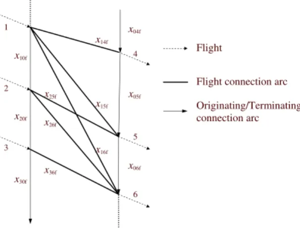
flights arrive or depart. In addition, an imaginary master source node and a master sink node are concep-tualized (not actually created) in the network to account for the beginning-of-the-day and the end-of-the-day effects. There are three types of arcs representing the different types of connections: theflight connection arcslink the arrival nodes to the departure nodes, theterminating(connection)arcslink the arrival nodes to the master sink node to represent aircraft arriving and remaining at the station for the rest of the day, and theoriginating(connection)arcslink the master source node to the departure nodes to represent the aircraft that are present at the station at the beginning of the day. All flight connections have to befeasiblewith respect to flight arrival and departure times; that is, the minimum turn-time has to be observed between the arrival flight and the following departure flight to allow for the connection. The binary decision vari-ables correspond to fleet types that cover these three types of connections at stations.Fig. 1, taken from

Abara (1989), illustrates the connection network for a station that includes 12 connections: six (feasible) flight connections, three connections from arrival flights to terminations, and three connections from orig-inations to departure flights.

Next, we introduce some notation to present AbaraÕs mathematical formulation. LetLbe the set of flight legs, indexed byiandj,Fbe the set of fleet types, indexed byf, andSbe the set of stations, indexed bys. Further, letAsandDsbe the respective sets of arrival and departure legs for stations,s2S. Definexijfto be a binary decision variable that takes on a value of 1 if the feasible connection between legi2Lto legj2L is covered by fleet type f2F, and is 0 otherwise. (The indices i= 0 andj= 0 denote originating and ter-minating arcs, respectively.) The three imperative constraints (cover, balance, availability) apply. The objective is to maximize the expected revenue less the operating cost. The benefit from using fleet type f for a connection is arbitrarily assigned as the benefit from the departing flight jof the connection, and is denoted aspjf, which is a comprehensive combination of profit, aircraft utilization, etc.Abara (1989)uses a nominal unit operating cost, denoted byc, for each assignment of the typex0jfthat initiates the use of a fleet typeffor some flight legj. In general, however, this cost factorccan be made fleet and flight leg spe-cific, and could be computed by combining the operating costs with the cost from spilled passengers that are estimated from the projected demands, recapture rates, fare structure, and available seats. The practice of calculating the cost is not universal within the industry. We will discuss this issue further in Section 5.1.

1 2 3 4 5 6 x14f x15f x16f x25f x26f x36f x10f x20f x30f x04f x05f x06f Flight

Flight connection arc Originating/Terminating connection arc

(5)

The mathematical program based on this connection network is given as follows:

Model 3.1. Basic fleet assignment model using a connection network

Maximize X i2L[f0g X j2L X f2F p_jfxijfc X j2L X f2F x0jf ð1aÞ subject to X i2L[f0g X f2F xijf¼1 8j2L; ð1bÞ X i2L[f0g xilf X j2L[f0g xljf ¼0 8l2L; f 2F; ð1cÞ X i2Ds x0if X i2As xi0f ¼0 8s2S; f 2F; ð1dÞ X i2L x0if 6Af 8f 2F; ð1eÞ xbinary: ð1fÞ

In this model, the cover constraint(1b)requires that each ﬂight is preceded by an arrival or an originat-ing arc that is covered by a ﬂeet type. The equality constraint can be relaxed asP_i₂_L_[f0g

P

f2Fxijf 61 8j2L,

if not all flights are required to be served, as inAbara (1989). The balance constraint(1c)assures the flow balance at each leg in the network for each fleet type. In addition, theschedule balanceconstraint(1d) en-sures that the same number of aircraft of each type remain at each station every night so that the same assignment can repeat daily. The availability constraint(1e)limits the number of aircraft used to Af, the number of aircraft available for typef. Other side-constraints such as a limit on the number of aircraft that stay overnight at each station can be added as needed.

In AbaraÕs solution approach, the constraints(1d) and (1e)are chosen to be ‘‘soft’’ constraints, and are relaxed with appropriate penalty functions added to the objective function. That is,(1d)induces a penalty term pertaining to the shortage of originating and terminating ﬂeet types at each station, while(1e)induces a penalty term pertaining to the number of extra aircraft used over the available aircraft. The objective thus maximizes the expected revenue minus the operating cost along with the penalties from the relaxed constraints.

As mentioned above, all feasible connections have to be specified in the network for this model. This ensures that all connections selected in a solution are feasible. As a result, however, the network can easily grow to an unmanageable size due to the large number of possible flight connections.Abara (1989)deals with this problem by specifying a limit on the number of connection variables that are considered for each flight.

Using a very similar model formulation,Rushmeier and Kontogiorgis (1997)employ some preprocess-ing techniques to solve the problem more effectively without havpreprocess-ing to specify feasible connections for each flight. In particular, they resort toconnecting complexesfor representing feasible connections whereby the operations at each station are partitioned into complexes such that each complex has an equal number of incoming and outgoing legs, and feasible connections exist only within the same complex.Rushmeier and Kontogiorgis (1997)also consider some additional crew-based side-constraints in their model. They design a heuristic to solve the problem in which the LP (linear programming) relaxation is first solved and the resulting solution is rounded to obtain an initial solution that is fed into a depth-first branch-and-bound process, which is run for a two-cpu-hour time limit. Seven problems having eight aircraft types, over 1600 legs, and nearly 100 stations were solved using this approach in concert with CPLEX 3.0 on an IBM RS-6000/590 workstation having 256 MB of RAM. Within the 2-hour limit, an average of 13 integer feasible solutions per run were discovered for these test problems.

(6)

3.2. Basic FAM using a time–space network structure

In contrast with the ‘‘connection network’’, the time–space network structure focuses on representing flight legs, and leaves it to the model to decide on the connections, as long as these are feasible to the time and space considerations. This provides a greater freedom for establishing connections, while reducing the number of decision variables because the number of flight legs is far lesser than the number of possible con-nections. AsRushmeier and Kontogiorgis (1997)point out, however, the time–space network is not able to distinguish among the specific aircraft on the ground, which limits its application in the subsequent routing problem. Moreover, the use of connection networks can facilitate a different class of branching decisions based on whether or not to select a particular fleet type to make a connection between a specific pair of flight legs. Nonetheless, beginning with Berge and Hopperstad (1993) andHane et al. (1995), who were among the first researchers to use this network structure, this time–space representation has largely become the method of choice in formulating the fleet assignment problem.

The time–space network representation superimposes a set of networks, one for each fleet type. This al-lows for fleet type-dependent flight-times and turn-times. If the flight- and turn-times are not significantly different among some particular fleet types, then a composite network representation can be constructed for these types. In each typeÕs network, each event of flight arrival or departure at a specific time is associated with a node. In order to allow for feasible aircraft connections, an arrival node is placed at the flightÕs ready-time, given by its arrival time plus the necessary turn-time, thus representing the time the aircraft is ready to take-off. There are three types of arcs in the network for each fleet type:ground arcsrepresenting aircraft staying at the same station for a given period of time,flight arcsrepresenting flight legs, and wrap-around arcs(orovernight arcs) connecting the last events of the day with the first events of the day, which, due to thesame daily schedule, replicate the first events of the following day. This ‘‘wrap-around’’ ensures continuity of the fleet assignment every day. Airport stations are also duplicated into multiple copies, one for each fleet type. In the sub-network for any given fleet type, anetwork time-lineis associated with each station, consisting of a series of event nodes that occur sequentially with respect to time at this station, along with the ground and wrap-around arcs that link these event nodes. The network time-lines of the same fleet type are connected by incoming and outgoing flight arcs to represent the flight-leg-based flows for that type. The requirement that only one fleet type is assigned to each flight leg jointly regu-lates the flows that occur in the networks of the different types, thus making all the networks interdependent.

Fig. 2depicts two stations in a time–space network for two fleet types. The time axis progresses down-ward through the figure, and each node representing a flight arrival or departure event at a particular sta-tion is posista-tioned vertically according to its time of occurrence. There are two stasta-tions A and B depicted in this figure and two fleet types (Type 1 and Type 2). The full arrows as defined in the figure pertain to the fleet of Type 1 and the broken or dashed arrows pertain to the fleet of Type 2. (Other details of this figure are explained in its legend.)

In the model formulation, the flow on any flight arc is represented by a binary decision variable that is restricted so that the corresponding flight leg is covered by only one type of aircraft. The flows on the ground arcs and the wrap-around arcs take integer values, which represent the number of aircraft of the corresponding type that continue to reside at the particular station. As usual, the formulation includes the three main constraints: cover, balance, and availability. A particular count time-lineis also specified in the network for counting aircraft, typically at an early time in the morning, say, 3 am EST, when the number of flight arcs is low. For each fleet type, the flows on all the corresponding flight and ground arcs that cross this time-line are summed to assure that the total number of aircraft of this type in use (at this time) does not exceed the number of available aircraft. The network flow balance constraints then ensure that the availability constraints are satisfied for all times in the network. We note here that because of the explicit wrap-around arcs and flow balance restrictions, the schedule balance constraints of Model 3.1 (see

(7)

(1d)) can be omitted from the formulation for the time–space network. The objective is to maximize the revenue or, equivalently, to minimize the assignment cost.

To be consistent with the existing literature as much as possible, we use the following notation through-out the remainder of this paper.

Notation

S set of stations in the network, indexed bys,o, ord F set of ﬂeet types, indexed byf

L set of flight legs scheduled, indexed bylor {odt}, whereo,d2Sandtdenotes the time when the flight takes off fromoor is ready atdfor the next take-off

N set of nodes in the network, indexed by {fst}, wheref2F,s2S, andtdenotes the event time O(f) set of arcs for ﬂeet typefthat cross the aircraft count time-line,f2F

cfl cost of assigning fleet typefto legl,f2F,l2L Af number of available aircraft for fleet typef,f2F xfl= 1; if fleet typef covers legl;f 2F; l2L

0; otherwise

(The decision variables xﬂcan also be denoted by xfodtforf2F, {odt}2L.)

yfstt0 ﬂow of aircraft on the ground arc from node {fst}2Nto node {fst0}2Nat stations2Sin ﬂeet

typefÕs network, forf2F, wheret0 >tin general, andt06_t_{for wrap-around arcs}

t,t+ the time preceding and succeedingt, respectively, in the time-line

Time Stations Station B Station A A1 B1 D1 B2 C1 F1 E1 10:00am 9:00am 12:00pm 11:00am A2 C2 D1 E2 F2

Arcs for Type 1 Arcs for Type 2

Wrap-around arcs for Type 1

(8)

The aircraft count time-line is used as a starting point for representing the series of events occurring in the network. The ﬁrst set of nodes after this time-line are denoted as {fst1},f2F,s2S, whereas the last set

of nodes of the day are denoted as {fstn},f2F,s2S. With this notation, we are ready to present the basic ﬂeet assignment model, proposed ﬁrst byHane et al. (1995):

Model 3.2. Basic fleet assignment model based on time–space network structure

Minimize X l2L X f2F cflxfl ð2aÞ subject to Cover: X f2F xfl¼1 8l2L; ð2bÞ Balance: X o2S xfostþyfstt X d2S xfsdtyfsttþ¼0 8ffstg 2N; ð2cÞ Availability: X l2OðfÞ xflþ X s2S y_fst nt1 6Af 8f 2F; ð2dÞ xbinary; yP0. ð2eÞ

As discussed above, constraints(2b), (2c), and (2d)are the cover, balance, and aircraft availability con-straints, respectively. Not surprisingly, solving FAP on a network consisting of hundreds of stations inter-woven by thousands of flights poses a challenging task. Indeed, Gu et al. (1994) have shown that this problem, even without the availability constraints, is NP-hard for three fleet types. Therefore, Hane et al. (1995) have proposed a series of preprocessing steps that aim to reduce the size of the network, and hence the computational effort. In the following, we review these preprocessing steps, which have now be-come a standard practice.

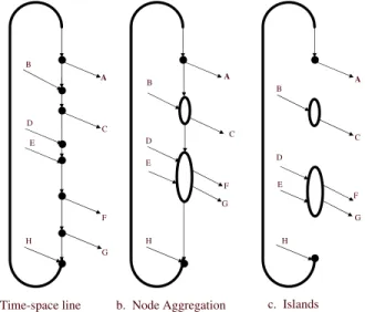
The ﬁrst preprocessing step is based on the observation that as long as the network represents the correct connections, the exact time pertaining to each nodeÕs event does not matter. Hence, consecutive arrivals and the subsequent consecutive departures can share a single node such that each arrival at the aggregated node can be feasibly connected to any departure at this node. This is callednode aggregation(a similar technique was adopted earlier byBerge and Hopperstad (1993)).Fig. 3illustrates this concept. Part (a) ofFig. 3 delin-eates a network time-line representation of a station for one type. Again, time increases downward in the vertical direction for representing the time of occurrence of each event (node). Part (b) demonstrates the node aggregation that can be performed for this station. Note that there are no more aggregation oppor-tunities available at this station. For example, arrival arc B cannot share the same node as departure arc A, since A departs earlier than B arrives, and thus a connection from B to A would be infeasible. The exper-iments byHane et al. (1995)show that node aggregation reduces the number of rows by a factor of 3–6 and the number of columns by a factor of 1–3 in their model.

The second preprocessing step is based on the observation that some stations, especially the spoke stations in hub-and-spoke configurations, have sparse flight activities, leaving no aircraft on the ground during certain periods of time. In this case, the ground arcs have zero flows and can therefore be deleted from the network. For each ground arc removed, there is another zero-valued ground arc, which is encountered after an equal number of arrivals and departures. This ground arc can also be removed. This simplification results in the cre-ation ofislandsin the time-line of the station. (This concept is similar to that ofconnection complexesdiscussed in Section 3.1.) InFig. 3, removing the zero-flow ground arcs from part (b) results in the islands shown in part (c). The third preprocessing techniqueeliminates missed connections. If two flights that must be flown con-secutively result in a missed connection when assigned to a fleet type, usually because of the longer turn-times for that fleet type, this pair of flights can be removed from that typeÕs network. InFig. 2, for example,

(9)

if ﬂight arcsC2 andB2 must be ﬂown consecutively, they would result in a missed connection, and so, these two arcs can be removed from Type 2Õs network.

These three preprocessing steps can considerably reduce the problem size. Indeed,Hane et al. (1995) re-port that the size of a typical problem instance is reduced from 48,982 rows and 66,942 columns to 7703 rows and 20,464 columns through these three steps. In addition, a combination of algorithmic strategies such as interior-point methods, dual steepest-edge simplex approach, and branching on cover constraints by prioritizing variables based on the objective coeﬃcientsÕranges, have been shown to signiﬁcantly reduce the overall computational requirements.

These basic ﬂeet assignment models have had a major impact on the airline industry. AbaraÕs (1989)

implementations have resulted in a 1.4% improvement in operational cost margins at American Airlines.

Rushmeier and Kontogiorgis (1997)report an annual beneﬁt of at least $15 million at US Airways, and the network processing techniques byHane et al. (1995)have been widely applied in the industry. These early achievements have inspired researchers to aim for further improvements to the FAM.

4. Integrated ﬂeet assignment models

Although the earlier literature reviewed in the previous section attempts to solve the FAP independently of the other airline decision processes, the FAP is, in fact, intricately interwoven with several related overall planning and operational contexts. The FAP depends on theflight schedulingprocess (also called schedul-ing/network design) that specifies the flight network, including the departure and arrival stations and times. The fleet type assignment information produced by the FAP is, in turn, fed into the aircraftmaintenance rout-ing(orrotation) process so that individual aircraft can be assigned specific routes among those prescribed for

B A C D E F G H B A C D E F G H H A D E B C F G

a. Time-space line b. Node Aggregation c. Islands

(10)

its own type, while satisfying maintenance constraints. Thecrew schedulingprocess is also dependent on the fleet assignment solution in that each crew member needs to be assigned to legs that are flown by the fleet types that he/she is qualified to fly. Furthermore, the revenue management and the fleeting decisions are also interdependent, since revenue management provides the FAP with the estimated revenue or profit parameters in the objective function, while the capacities assigned by FAP restrict the actual revenue realization. Each of these problems, by itself, constitutes an interesting topic for research. We refer the interested reader to several survey papers for more information on these problems; see, for instance,Gopalan and Talluri (1998)for the general airline scheduling process;Barnhart et al. (2003)for the crew scheduling problem; andYu and Yang (1998)andBarnhart et al. (2004)for applications in revenue management, scheduling processes, along with other studies in the airline industry, such as traffic control.

Clearly, a main drawback of solving these problems sequentially, and thus separately, is that an optimal solution for one problem is not necessarily optimal for the entire system, and can even yield an infeasible input to the subsequent processes. The interdependence between these processes have motivated researchers to focus on integrated models that simultaneously consider several of these problems so as to achieve a bet-ter solution for the entire system. Although no attempts have been made to integrate all the above-men-tioned planning processes due to the potential intractability of the resulting model, various integrated models of two or more sub-problems have been proposed, together with solution techniques that have gen-erated optimal or near-optimal solutions and higher revenues for the airlines. In this section, we review such integrated FAM models: Section 4.1 describes the FAM integrated with schedule design, while Section 4.2 examines the FAM integrated with maintenance routing and crew scheduling.

4.1. FAM integrated with schedule design

Schedule design is usually the first step in the airline operations planning process. It determines the flight network, including flight departure times and departure/arrival stations. The basic fleet assignment models discussed above are then solved based on this network with fixed flight departure times.

Clearly, an integrated fleet assignment and flight scheduling model can increase revenues by allowing for improved flight connection opportunities in the FAP. This is the stance adopted byDesaulniers et al. (1997)

andRexing et al. (2000), who assume that the flight origin–destination information is given, but they allow the flight departure times to vary within certain time-windows, thus resulting in different connection pos-sibilities for the FAP. Denoting the departure time-window for legi,i2L, as [aif,bif], the necessary turn-time from legito legj,i2L,j2L, asdijf, and letting the variableTifbe the realized departure time of flight legi flown by fleet typef,i2L, f2F, Desaulniers et al. (1997)add the following two constraints to the model ofAbara (1989)using a connection network:

aif 6Tif 6bif 8f 2F 8i2L; ð3aÞ

xijfðTif þdijfTjfÞ60 8f 2F 8i;j2L: ð3bÞ

However, the inclusion of the nonlinear constraints(3b)lends computational diﬃculty and inhibits the modelÕs practical use. Alternatively, using a suitable large numberM,(3b)can be reformulated as

Tifþdijf Mð1xijfÞ6Tjf 8f 2F 8i;j2L; ð3cÞ

as used variously in vehicle routing models (Desrosiers et al., 1983; Kohl and Madsen, 1997).

In the model proposed byRexing et al. (2000), similar toLevin (1971)(who has considered a single-fleet-type model), the set of departure times for each leg is discretized within its specified time-window and each possible departure time is represented by a copy of the flight arc, so as to accommodate the different depar-ture time possibilities in the time–space network. For the purpose of implementation, they use time-win-dows of durations 20 and 40 minutes, in which copies of legs are created for every 5- and 1-minute

(11)

intervals, respectively. Obviously, only one of these copies needs to be covered by a fleet type. The resulting changes to the basic model formulation presented in Section 3.2 are straightforward: Each variablexflis replaced withP_n₂_N_flxnfl, whereNfldenotes the set of arc copies of leglin fleet type fÕs network, and the

binary variablexnfltakes the value of 1, if copynof leglis covered by fleet typef, and equals 0 otherwise. Although this representation allows for fleeting flexibility, the inclusion of several copies of each arc in the formulation naturally increases the number of decision variables, and hence, the problem size. Two solution approaches are proposed byRexing et al. (2000): a direct solution technique (DST), which simply uses a commercial package to solve the preprocessed problem, and an iterative solution technique (IST), which we describe in detail below. In both approaches, the network is preprocessed by applying node aggre-gation and island formation techniques as described in Section 3.2. In addition,redundant arcsthat stem from the existence of multiple copies of arcs are identified and deleted, whereby all arcs pertaining to the same leg, having the same cost, and sharing the same tail node are dominated by the earliest such one in the time-line. Thus the remaining copies of such arcs can be removed from the network. This pre-processing step of eliminating redundant arcs reduces the problem size by respectively 40% and 66% for sample problems having 5- and 1-minute time intervals within respective time-windows of 20 and 40 min-utes. The node aggregation step is shown to further reduce over 80% of the rows and about 56% of the columns. Furthermore, problems using islands are solved 10–20% faster than those without islands.

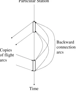
For the purpose of solving relatively larger practical sized problems, an iterative solution technique (IST) is proposed that is more robust and has lesser memory requirements. In this approach, a master problem and a group of sub-problems are solved iteratively, where the master problem searches for ‘‘super-optimal’’ solutions and the sub-problems check for feasibility. The master problem is formulated by replacing the set of arc copies belonging to each leg with a single arc having areduced duration, which departs at the end of the departure time-window and arrives at the start of the arrival time-time-window. Because of the existence of the reduced-duration arcs, the optimal solution to the master problem provides a lower bound to the original problem. The feasibility of this solution is then checked by formulating a sub-problem for each fleet type using the original network with time-windows, including only copies of flight arcs that are assigned to this fleet type in the master problem, and adding backward connection arcs that link the later arrivals with the earlier departures at the same station (see

Fig. 4). Then, zero costs are associated with the flight arcs and positive penalty costs with the backward arcs, and the new network is solved to minimize the penalty costs on the backward arcs. If the solution yields a zero objec-tive value, then the master problem is feasible for this fleet type. Otherwise, some flight ‘‘back-ups’’ are neces-sary. The flights that are connected by the backward arcs are identified as the ‘‘problem flights’’, of which the reduced-duration arcs are replaced by their original copies within the corresponding time-windows. This up-dated network is passed back to the master problem for the next iteration. The master problem solution yields an optimal assignment when no problem flights arcs are identified in the sub-problems.

Numerical experiments conducted byRexing et al. (2000)suggest that the IST algorithm performs better than the DST when the time-windows are narrow. However, it is not a good choice when the time-windows are wide (e.g. 40 minutes), since the reduced-duration arcs from the master problem yield many infeasible solutions, and so, several more iterations are typically required.Rexing et al. (2000)report that this extra departure time ﬂexibility added to the FAP results in a cost saving of over $20 million annually for 20-min-ute time-windows, and even more for 40-min20-min-ute time-windows. A further integration of scheduling and ﬂeeting certainly deserves more investigation.

If a tentative flight schedule is at hand that includes certain optional legs, then the decision on which optional legs to offer can be made concurrently with the FAM. Changes in the schedule naturally affect demands. For example, the deletion of a leg may increase the demands on paths having origins, destina-tions, and time-frames that are compatible with the original paths that contain the particular leg. Therefore, in order to determine the set of optional legs to offer, we need to consider the revenue changes due to the deletion of paths (caused by the deletion of optional legs on these paths). This idea was proposed by Loha-tepanont and Barnhart (2004), in which leg selection decisions and FAM are integrated.

(12)

In addition to the notation used in Section 3.2, the following notation is needed to incorporate the leg selection decision into the FAP, as proposed byLohatepanont and Barnhart (2004).

P set of all paths, indexed byi

PO set of paths containing the optional legs (hence, subject to deletion), indexed byi LF set of mandatory legs, indexed byl

LO set of optional legs that are candidates for deletion, indexed byl L(i) set of legs on pathi,i2P

ri incremental revenue loss if pathiis excluded from the ﬂight network,i2PO zi= 1; if pathiis included in the flight network;i2P

O

0; otherwise

Model 4.1. Integrated leg selection and fleet assignment model

Minimize X l2L X f2F cflxflþ X i2PO rið1ziÞ ð4aÞ

subject to balance (2c); availability (2d); plus: ð4bÞ

X f2F xfl¼1 8l2LF; ð4cÞ X f2F xfl61 8l2LO; ð4dÞ zi X f2F xfl60 8i2PO; l2LðiÞ; ð4eÞ zi X i2LðiÞ X f2F xflP1 jLðiÞj 8i2PO; ð4fÞ ðx;zÞbinary; yP0: ð4gÞ Copies of flight arcs Backward connection arcs Particular Station Time

(13)

Notice that the cover constraints(2b)are split into(4c) and (4d)to distinguish between the mandatory and optional leg sets. Constraint(4e)ensures that if any leg is excluded from the network, then the path that contains the leg will be excluded, and(4f)ensures that if all the legs contained in a path are included in the network, then the path that contains them is also included. The work by Lohatepanont and Barnhart (2004) also describes detailed calculations for the revenue changes associated with the deletion of a leg. We will discuss this feature in Section 5.1 where we address other related cost considerations.

We note here that ifLF=;, then this model would serve the purpose of designing the entire ﬂight sche-dule, which is also the idea inYan and Tseng (2002), whose model integrates the scheduling process with ﬂeet assignment, while including path-based demand considerations. Details of this model are also included in Section 5.1.

4.2. FAM integrated with maintenance, routing, and crew considerations

To assure safety, aircraft need to undergo regular maintenance checks. FAA requires four types of main-tenance checks, labeled A, B, C, and D. Among them, the C and D types of checks take longer than 24 hours. FAM deals with these two types of checks by simply reducing the number of available aircraft during the times when some aircraft are scheduled for these maintenance checks. For the other two types of checks, the A checks take around 4 hours, and the B checks take 10–15 hours to perform. These checks can therefore be included in a more realistic, expanded formulation of the FAM.

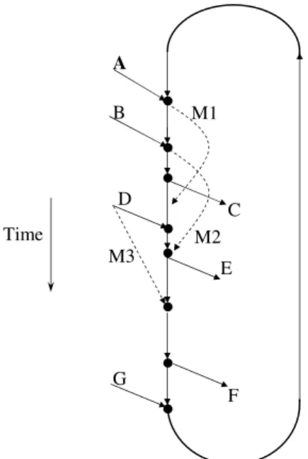
Clarke et al. (1996)classify the A and B checks as theshort maintenanceand thelong maintenancechecks, respectively, and include these maintenance constraints in Model 3.2. For this purpose, they add two types of maintenance arcs, one for each maintenance check, in the time–space network. Aircraft that are sched-uled to undergo maintenance checks in-between their ﬂight tasks should be assigned to these mainte-nance arcs (see Fig. 5for an example). Two corresponding lists are also constructed for these scheduled

B A C D E M1 F G M3 M2 Time

(14)

maintenance activities. They include, for each maintenance activity, the number of aircraft required, the maintenance station, the aircraft type, the maintenance time-window (i.e., the earliest starting time and the latest completion time for that maintenance activity), and its expected duration. If a ﬂight arrives at a maintenance station after the earliest starting time of the corresponding time-window and a long main-tenance can be completed within the time-window, then a leapfrog arcis created, which departs from the arrival event node and arrives at the same station after the corresponding maintenance duration (see arcs M1 and M2 inFig. 5). Multiple leapfrog arcs can be created for a maintenance activity, depending on the time-window and the duration of the maintenance service. For example, arcs M1 and M2 inFig. 5 corre-spond to the same maintenance activity.

LetPLdenote the set of long maintenance activities, indexed byp, and for activityp2PL, letMpbe the number of aircraft required to undergo long maintenance andJ(p) be the set of eligible leapfrog arcs, in-dexed byj. Furthermore, letmpjbe the number of aircraft taking arcj2J(p). Then, the long maintenance constraints can be stated as

X

j2JðpÞ

mpj¼Mp 8p2PL: ð5Þ

Note that similar to the ground arcs, the leapfrog arcs also participate in the network ﬂow balance con-straints(2c)as well as in the aircraft availability constraints(2d).

The duration of each long maintenance arc is, generally, longer than half of its allocated time-window length. This ensures that no aircraft can take more than one long maintenance arc—corresponding to the same requirement—in a row. (For example, inFig. 5, if the duration for M1 were shorter than half of its time-window, then it could ﬁnish before M2 even starts, which might result in an aircraft being assigned to two successive identical maintenance operations.)

On the other hand, most short maintenance requirements can be met simply by having the aircraft stay overnight at a maintenance station. This leads to the following set of constraints:

X

s2CMðfÞ y_fst

nt1PNMðfÞ 8f 2F; ð6Þ

whereCM(f) is the set of stations that can perform the required maintenance check for typef, andNM(f) is the average number of typefaircraft that need short maintenance. There are circumstances, however, in which simply counting the number of aircraft is not sufficient to ensure the required maintenance restric-tions for each aircraft. Some modificarestric-tions in the network are thus needed. Unlike long maintenance checks, however, short maintenance checks are not necessarily longer than half of their time-windows. Thus, particular attention should be paid to prevent double-counting. For this purpose, each flight arc that can be followed by a short maintenance check is split into two arcs: one is the real flight arc, and the other is the flight arcextendedby the duration of the short maintenance requirement (see arcsDand M3 inFig. 5). The cover constraints(2b)in Model 3.2 are thus transformed to ensure that for each flight leg, either its real flight arc or its extended flight arc is covered by an aircraft type:

X f2F xflþ X f2F X p2PS xmpfl ¼1 8l2L; ð7Þ

wherePSdenotes the set of short maintenance activities, and wherexmpflis a binary variable that takes the value of 1 if fleet typefflying leglundergoes maintenancep, and equals 0 otherwise. The variablexmpflis ascribed a smaller objective coefficient than xfl "f2F, l2L, in order to encourage more maintenance services.

This construct, however, signiﬁcantly increases the number of integer variables in the problem. Alterna-tively, leapfrog arcs can be added following the arrival ﬂights at the beginning of their short maintenance time-windows. Constraints(7) then revert to the usual cover restrictions(2b)for the legs associated with

(15)

such leapfrog arcs. Because the earliest time that double-counting can occur is after the end of the first leap-frog arc, the extended split flight arcs are applied instead of leapleap-frog arcs after the end of the first leapleap-frog arc to avoid the double-counting phenomenon. The maintenance constraints then transform to (in notation analogous to that defined before):

X

j2JðpÞ

ðmpjþxmpjÞ ¼Mp 8p2PS; ð8Þ

wherexmpjis a binary variable that takes the value of 1 if arcj,j2J(p), undergoes maintenancep, and equals 0 otherwise, and where the setJ(p) now includes the extended split ﬂight arcs, along with the leap-frog arcs, which are created for maintenance activityp2PS.

Clarke et al. (1996)also integrate some crew scheduling considerations into the FAP by attempting to limit the number oflonely overnights. This occurs when a crew, which arrives at a non-base station, has to stay overnight at this station because there is no departing aircraft that it is qualiﬁed to ﬂy on the same day after the minimum legal rest time. Such overnight rests at non-base stations are very expensive in terms of crew costs. Hence, Clarke et al. (1996) attempt to reduce the time-away-from-base for crews, using a structure similar to the leapfrog arcs.

Using these constructions and the callable library OSL, Release 2,Clarke et al. (1996)solve their model using an LP-based branch-and-bound algorithm, adopting the dual steepest-edge simplex method, and a special ordered set (SOS) branching mechanism, in which the decision variables are prioritized by the type capacity. They are able to thus solve problems involving up to eleven ﬂeet types and 2500 ﬂight legs within 2–5 hours of cpu time on an IBM RS/6000 model 550.

At Delta Air Lines,Subramanian et al. (1994)have incorporated maintenance issues into Coldstart, the ﬂeeting model of Delta, via the use of maintenance arcs in the time–space network, along with the consid-eration of lonely overnights. They report a projected savings of $300 million over the initial three years of applying the Coldstart model. However, no related modelling details are provided in the open literature.

Other integrated routing and ﬂeet assignment models include those proposed byDesaulniers et al. (1997)

andBarnhart et al. (1998). Both models use the idea of pre-specifying sequences of flights and assigning these sequences to fleet types, and adopt similar branch-and-price schemes, which utilize column generation to provide improved sequences. The difference between the two models is that the one proposed by Barn-hart et al. (1998)explicitly accommodates maintenance considerations using ground arcs, while the model ofDesaulniers et al. (1997)includes time-windows in the sub-problems using up to two copies of each turn arc. In the following, we use the string-based model ofBarnhart et al. (1998)to illustrate the basic concept in these two models. This string-based MIP model solves the weekly (or any cyclic) fleet assignment and aircraft routing problems simultaneously. The basic idea is to pre-specify sequences of maintenance-feasible legs between maintenance stations that satisfy the flow-balance constraints, and assign thesesequences (in-stead of single legs) to fleet types. Each such maintenance-feasible sequence is defined as an augmented string, which is a flight sequence (string) that is extended at the end of the last leg to include the maintenance time at a maintenance station. Thus, upon completing the assignment, a feasible aircraft maintenance rout-ing is at hand.

At each maintenance station, events of arrivals (i.e., maintenance completions) and departures are sorted in increasing order of time. Letef_l_;_aandef_l_;_ddenote the events of arrival and departure, respectively, of leglat a maintenance station, for ﬂeet typef,f2F. The superscripts ‘‘’’ and ‘‘+’’ are used to respectively represent the previous and succeeding events. Additionally, the following notation is used in the string-based FAM: SG set of augmented strings, indexed bys

SG_l set of augmented strings ending with legl,l2L SGþ_l set of augmented strings starting with legl,l2L Gf set of ground arcs in ﬂeet typefÕs network,f2F

(16)

als 1; if leglis in augmented strings;l2L;s2SG 0; otherwise

pf_j 1; if ground arcjcrosses the count time-line;j2G f_;_f ₂_F 0; otherwise

rf

s number of times that augmented strings, assigned to typef, crosses the count time-line,s2SG, f2F

xf s

1; if augmented string sis flown by fleet typefðat costcf

sÞ;f 2F;s2SG 0; otherwise

yf_j number of aircraft of typefon the ground arcj,j2Gf,f2F. (The decision variableyf_j can also be denoted byyf_ð_e_;_e0_Þ, whereeande0are, respectively, the starting and ending events of the ground arc

(e,e0₎₂_Gf ,f2F)

The string-based ﬂeet assignment and routing model can then be stated as follows:

Model 4.2. String-based fleet assignment and routing model

Minimize X s2SG X f2F cf sx f s ð9aÞ subject to X s2SG X f2F alsxfs ¼1 8l2L; ð9bÞ X s2SGþ_l xf s y f ðe_l_;_d;f;ef_l_;_dÞþy f ðef_l_;_d;eþ_l_;_d;fÞ¼0 8l2L; f 2F; ð9cÞ X s2SG l xf_s yf ðe_l_;_a;f;ef_l_;_aÞþy f ðef_l_;_a;eþ_l_;_a;fÞ¼0 8l2L; f 2F; ð9dÞ X s2SG rf_sxf_s þX j2Gf pf_jyf_j 6Af 8f 2F; ð9eÞ xbinary; yP0: ð9fÞ

In this model,(9b) and (9e)respectively represent the usual cover and availability constraints. Also, no-tice that instead of focusing on the nodes to maintain the conservation of flow, flow balance is enforced at the first and the last legs of augmented strings, as shown in constraints(9c) and (9d).

Along with the advantage of solving the assignment and routing problems simultaneously, comes the diﬃculty associated with the large number of strings, which is exponential in the number of legs. As a result,

Barnhart et al. (1998)develop a branch-and-priceapproach, in which an LP relaxation is solved at each node of the branch-and-bound tree using column generation (via the ‘‘pricing’’ sub-problem). In this algo-rithm, the pricing sub-problem is cast as aresource-constrained shortest path problemover a maintenance connection network, resembling that ofAbara (1989), in which the nodes represent the flights and the arcs represent the connections between flights at the same station. A maximum allowable flying time or elapsed time between successive maintenance operations is considered as a ‘‘resource’’, and each node and arc in a path respectively consumes this resource by the amount of flying hours and elapsed hours. For maintenance stations, the connection arcs are extended to include the maintenance time. The shortest path problem is solved for each fleet typef. If the shortest path, which in effect determines the reduced cost of the most enterable column with respect to the current LP basis, has a non-negative value for eachf, then an optimal LP solution is at hand; otherwise, new columns are generated from strings yielding negative values, and these are added to the master problem in the column generation process.

(17)

Using the node and island preprocessing techniques and implementing this branch-and-price approach, good solutions having an optimality tolerance ranging from 0.25% to 1.0% were achieved in about 5 hours on an IBM RS-6000/370 using CPLEX 3.0, for a 7-day, 1,124-ﬂight schedule covering 40 stations and hav-ing nine ﬂeet types, containhav-ing a total of 89 aircraft.

Based on this type of a string-based model,Rosenberger et al. (2004)propose a robust FAM that creates rotation cycles(i.e., sequence of legs assigned to each aircraft) that are short and that involve as few hub stations as possible, so that flight cancellations or delays will have a smaller chance to cascade into a large number of subsequent stations, particularly hubs. In their network, only the time-lines associated with hub stations are included. A string that starts and ends at the same hub is called acancellation cycle, and a string that starts and ends at different hubs forms anacyclic string. A network having more cancellation cycles and less acyclic strings is shown to be more robust. As the number of legs in the set of acyclic strings de-creases, a lower bound on the number of cancellation cycles increases. Consequently, two alternative mod-els are formed based on the string-based FAM. Both formulations share the same constraints of those in Model 4.2. The first model imposes an upper bound on the number of legs in acyclic strings while minimiz-ing the total cost, and the second model minimizes the number of legs in acyclic strminimiz-ings while constrainminimiz-ing the total cost by an upper bound.

5. Fleet assignment models with additional considerations

In addition to the integration efforts discussed in the previous section, researchers have also started relaxing some of the restrictive assumptions made in the basic FAM described in Section 3. In this section, we present some of these efforts. Specifically, Section 5.1 describes an FAM that incorporates path-based demands into the fleeting. Section 5.2 presents a weekly fleeting model. A neighborhood search approach for an FAM that involves through-flight decisions is introduced in Section 5.3. Finally, Section 5.4 dis-cusses some other non-optimization approaches for fleeting problems.

5.1. FAM including passenger considerations

The FAM formulations that we have introduced thus far minimize the total fleeting and spill costs (or maximize the profit), considering a cost term for each possible leg-fleet type combination in the objective function. These costs are calculated based on the corresponding fleet type capacity and the forecasted leg demand. However, a significant portion of all demands flown by US airlines consists ofmultiple-leg pas-sengers(i.e., passengers whose itineraries are comprised of more than one leg), especially under the hub-and-spoke network structure, in which passengers typically fly into and out of hub airports in between their origins and destinations. Clearly, the demand coming from a multiple-leg passenger will be dependent on the availability of seats on all the involved legs (this is called the ‘‘network effect’’). Thus, (i) leg demands can be highly dependent, and (ii) passengers who demand to fly on a particular leg arenot identicalin terms of the revenue that they will generate and the airline resources that they will consume. Therefore, some re-cent fleet assignment approaches have included the network effect consideration (see, for exampleJacobs et al., 1999). Furthermore, passengers, who fail to get their requested itinerary, can sometimes be routed to other similar paths (the ‘‘recapture effect’’), making path demands dependent.

Traditionally, an isolated path-based passenger decision model (referred to as the ‘‘passenger mix’’ mod-el in the literature) is solved after the FAM, so as to determine which passengers to accept on each leg, given the capacity assigned to each leg as well as path-based demands.Glover et al. (1982), Dror et al. (1988), Phillips et al. (1991), Farkas (1995), Kniker (1998), andTalluri and Van Ryzin (1999)present various ver-sions of the passenger mix model. Below, we present a passenger mix model proposed byBarnhart et al. (2002), which minimizes the loss of revenue due to spills. Consider the following notation:

(18)

P set of paths in the ﬂight schedule, indexed byiorj P(l) set of paths inPthat contain legl,l2L

li mean demand on pathi,i2P

farei estimated fare price on pathi, given by the weighted average of the diﬀerent fare-classes, based on the estimated proportion of each fare-class on that path,i2P

g

Cap_l capacity assigned to legl,l2L

bj_i recapture rate; i.e., the fraction of customers spilled from pathitoward pathjthat aresuccessfully captured on pathj,i2P,j2P,j5i

tj_i number of passengers spilled from pathiwho are redirected to (but not necessarily accepted on) pathj,i2P,j2P,j5i

t_i number of passengers spilled from pathithat are not recaptured on any other paths,i2P

Barnhart et al. (2002) calculate the recapture rate,bj_i, using thequality of service index (QSI) (Kniker, 1998), which represents the ‘‘attractiveness’’ of each path with respect to all other paths. Denoting the QSI for path j as qj and the total QSI for all the paths in the market as Q, bj

i is calculated as qj

1Qþqj

"i5j, and is set to 1 fori=j. Their proposed formulation can be represented as follows:

Minimize X

i2P

½fare_it_i þ X j2P:j6¼i

ðfare_ibj_ifare_jÞtj_i ð10aÞ

subject to Capg_lþ X i2PðlÞ ðt_i þ X j2P:j6¼i tj_iÞ X i2P X j2PðlÞ:j6¼i bj it j iP X i2PðlÞ l_i 8l2L; ð10bÞ t_i þ X j2P:j6¼i tj_i 6_l i 8i2P; ð10cÞ tP0: ð10dÞ

The total lost revenue because of spill isP_i₂_Pðfare_it

i þ

P

j2P:j6¼ifareit j

iÞ, while the regained revenue

be-cause of recapture isP_i₂_PP_j₂_P_:_j_6¼_ibj_ifare_jtj_i. The diﬀerence between these two terms is the net revenue loss due to spillage, which is to be minimized in the objective function. In the capacity constraints (10b), for each legl, the termP_i₂_P_ð_l_Þðt_i þP_j₂P:j6¼it

j

iÞis the number of passengers who have requested but are spilled

from the paths that contain legl, and the termP_i₂_PP_j₂_P_ð_l_Þ_:_j_6¼_ibj_itj_i is the number of passengers recaptured from other paths to the ones that contain legl. The diﬀerence between these two terms is the net spillage from leg l. Therefore, constraints(10b) require that the capacity assigned to any leg cannot be less than the total demand on paths containing this leg minus the net spillage from this leg. Constraints(10c)are the demand constraints, which ensure that the spillage from pathidoes not exceed the demand on this path.

Integrating(10)with the FAM yields the path-based ﬂeet assignment model proposed byBarnhart et al. (2002).

Model 5.1. Path-based fleet assignment model

Minimize X l2L X f2F cflxflþ X i2P fare_it_i þ X j2P:j6¼i ðfare_ibj_ifare_jÞtj_i " # ð11aÞ

subject to cover (2b); balance (2c), availability (2d); plus: ð11bÞ

X f2F Cap_fxflþ X i2PðlÞ t_i þ X j2P:j6¼i tj_i ! X i2P X j2PðlÞ:j6¼i bj it j i P X i2PðlÞ li 8l2L; ð11cÞ t_i þ X j2P:j6¼i tj_i 6_l i 8i2P; ð11dÞ xbinary; ðy;tÞP0: ð11eÞ

(19)

Note that the capacity constraints(11c)are the key restrictions that link the two separate decision pro-cesses together.

Because of the network effect, the inclusion of such demand management decisions greatly increases the size and complexity of the problem.Barnhart et al. (2002)propose a heuristic solution technique for this formulation that is based on considering a restricted set of columns generated by the LP relaxation. Spe-cifically, this approach first omits constraints(11d)from the model, as they are usually not binding. A coef-ficient reduction technique is applied to constraints (11c) for which Cap_f >P_i₂_P_ð_l_Þli. This coefficient

reduction scheme is more effective when the recapture effects are not considered. The LP relaxation is then solved based on a column and row generation technique, where the columns are generated for spill vari-ables having negative reduced cost, and rows are generated for violated constraints (11d). The resulting model having the generated columns is then solved via a branch-and-bound procedure for determining an integer solution. Their computational experiments using networks having up to 2044 legs and 76,641 paths suggest that incorporating both the network and recapture effects can significantly impact the reve-nue. Using path-based demand alone yields an annual revenue increase of over $30 million, and including the recapture effect yields another $2–$115 million (in the order of a total of $33.7 million to $153.2 million per year) for a major US carrier.

Recall that in Section 4.1, we presented Model 4.1 that simultaneously performs the ﬂeet assignment and leg selection decision, considering a set of optional legs, where this model utilizes an estimate of the revenue diﬀerence resulting from the deletion of a leg. We are now ready to calculate the value of this revenue dif-ference. When pathj, j2PO, is deleted from the schedule (due to the deletion of a leg in the path), the direct revenue loss from pathjwill befarejlj. However, some customers may choose to select another path, sayi2P, thus increasing the demand on path i. LetDli

jbe a demand correction term that denotes the

incremental demand on path i when path jis excluded from the network. Correspondingly, the revenue gained on pathibecause of this demand increase is fare_iDli

j. Thus, the net revenue loss due to the

elimi-nation of pathjis given byfare_jlj

P

i2P:i6¼jfareiDlij. Using this new term in the objective function,

Loha-tepanont and Barnhart (2004)propose to integrate the leg selection decision of Model 4.1 into Model 5.1 as follows:

Model 5.2. Integrated leg selection and path-based fleet assignment model

Minimize X l2L X f2F cflxflþ X i2P fare_it_i þ X j2P:j6¼i ðfare_ibj_ifare_jÞtj_i " # þX j2PO fare_jl_j X i2P:i6¼j fare_iDli j ! ð1zjÞ ð12aÞ

subject to constraints (4b)–(4f) from Model 4.1; plus: ð12bÞ

X i2PðlÞ X j2PO Dli jð1zjÞ þ X f2F Cap_fxflþ X i2PðlÞ t_i þ X j2P:j6¼i tj_i ! X i2P X j2PðlÞ:j6¼i bj_itj_iP X i2PðlÞ l_i 8l2L; ð12cÞ X j2PO Dli jð1zjÞ þti þ X j2P:j6¼i tj_i 6_l_i 8i2P; ð12dÞ ðx;zÞbinary; ðy;tÞP0: ð12eÞ

In constraints (12c) and (12d), the terms P_i₂_P_ð_l_ÞP_j₂_PODli_jð1zjÞandPj2PODli_jð1zjÞ are the

(20)

Model 5.2 is solved using the same heuristic approach proposed for Model 5.1. One additional dif-ficulty of solving Model 5.2 arises due to the estimation of demand correction terms. The demand parameters and the demand correction terms used in the model are estimated via a schedule evaluation package that takes flight schedules as input. Therefore, evaluating demand requires a large number of runs using the package corresponding to all combinations of schedules. To avoid this, demands and de-mand correction terms are estimated and revised iteratively using the schedule obtained from Model 5.2 along with the schedule evaluation package. Specifically, the demand for the full schedule including all the mandatory and optional legs obtained from the schedule evaluation package are chosen as the initial set of demand estimates. Then, at each iteration, the heuristic approach used for Model 5.1 is applied to solve Model 5.2, using the current demand estimates. The resulting schedule is input to the schedule evaluation package to obtain a new set of demand estimates. These estimated demands are then used to evaluate the revenue by solving a passenger mix model due toKniker (1998), similar to the one pre-sented in(10). The resulting objective value of this passenger mix model is a maximum schedule revenue. At the end of each iteration, if the difference between this revenue and the estimated revenue obtained from Model 5.2 falls below a pre-specified threshold, or, alternatively, if the solutions produced by Mod-el 5.2 over two consecutive iterations are close enough, then the process is terminated. Otherwise, the paths having inaccurate revenue estimates obtained from Model 5.2 are identified, and the associated demand correction terms are revised based on the set of demand estimates obtained from the schedule evaluation package earlier in the iteration, and the iterations continue using the updated demand correc-tion terms.

Due to the large size of Model 5.2, solving it even with the heuristic proposed for Model 5.1 takes several days. To be able to obtain a solution in a more realistic time-frame, an approximate model is developed by

Lohatepanont and Barnhart (2004), in which all demand correction related terms are dropped, resulting in a Model 5.1 type of formulation except that the cover constraints are split as in(4c) and (4d)to treat the sets of mandatory and optional legs separately. Meanwhile, recapture rates are also adjusted to compensate for the effects of schedule changes over demand. When the demand correction terms are present, the recap-ture rates purely reflect the percentage of passengers that are accommodated by some alternative paths when the capacities on their desired paths are constrained. Now that the demand correction terms are ab-sent, the recapture rates need to also reflect the re-accommodation of passengers from the deleted paths to the remaining paths. Therefore, the set of adjusted recapture rates will be different than the ones calculated using QSI, and are accordingly adjusted iteratively in the same manner as the demand correction terms are adjusted at the end of each iteration, while the stopping criteria are not met. The original (unadjusted) re-capture rates are used as the initial values for the adjusted ones. Two practical-size problems are solved using this approach, and yield an annual revenue increase of $147.5 million and $360.6 million, respectively.

Yan and Tseng (2002) consider passenger demands in their integrated scheduling and fleeting model from a different perspective. Instead of defining passengersÕpaths to include specific legs, they consider their origins and destinations (O–D pairs), and leave it to the model to select the legs for composing passengersÕ routes. They resort to two groups of networks. The first group includes the fleet-flow time–space networks, one constructed for each fleet type, where flight arcs are all optional and a decision needs to be made on which ones to select to include into the schedule. The second group of networks are the passenger-flow time–space networks, one for each O–D pair. These networks containdelivery arcs and hold arcs, which are copies of the flight arcs and ground arcs, respectively, from the fleet-flow time–space networks. In addi-tion, the passenger-flow time–space networks containdemand arcs, each starting from the passengerÕs des-tination station and arrival time, and ending at the origin station and departure time. The flow upper bounds on these arcs are the forecasted demands. The reason for the particular orientation of these demand arcs is to conserve passenger flows in the network. We use the following notation to present the model by

(21)

OD set of O–D pairs, and thus, the set of passenger-ﬂow networks, indexed by {od} orp

PNp set of nodes in the passenger-ﬂow network for O–D pairp, indexed by {st}p, wheres2S,tdenotes the event time, andp2OD

DA set of demand arcs indexed bya or {dot}, where {od}2OD andtdenotes the event time (recall that each demand arc is from the destination station to the origin station)

e

la mean demand on demand arca,a2DA

g

farea average fare on all paths that can contribute to the demand on arca,a2DA Darca ﬂow on demand arca,a2DA

Larcp_l ﬂow on delivery arclin network p,l2L,p2OD

Harcp_stt₀ ﬂow on the hold arc from node {st}pto node {st0}p, where {st}p, {st0}p2PNp,p2OD

The following formulation is based onYan and Tseng (2002), and is modiﬁed for the purpose of con-sistency in presentation:

Model 5.3. Integrated scheduling and FAM with passenger demand considerations

Minimize X l2L X f2F cflxfl X a2DA g

fare_a Darca ð13aÞ

subject to balance (2c) and availability (2d); plus: ð13bÞ

X f2F xfl61 8l2LO; ð13cÞ X d2S: fsdg¼p Darcdstþ X s02S: s0_6¼_s Larcp_s0_stþHarcp_st_t X o2S: fosg¼p Darcsot X s02S s0_6¼_s Larcp_ss0_tHarc p sttþ¼0 8fstgp2PNp; p2OD; ð13dÞ X p2OD Larcp_l 6X f2F Cap_fxfl 8l2L; ð13eÞ Darca6ela 8a2DA; ð13fÞ Larcp_l6_max f2F Capf 8l2L; p2OD; ð13gÞ

xbinary; ðy;Larc;Darc;HarcÞP0: ð13hÞ

Yan and Tseng (2002)also consider ground-holding costs for they-variables and passenger waiting costs for theHarc-variables in the objective function, in addition to terms given in(13a)above. Constraints(13d)

ensure flow balance in the passenger networks. Constraints(13e) enforce the capacity restriction on the number of passengers accepted on each legl2L. These are the very constraints that link the fleet-flow net-works and the passenger-flow netnet-works. Constraints(13f) and (13g)set upper bounds on the demand arcs and the delivery arcs as given by the projected demands and the maximum aircraft capacity, respectively. Notice that although the capacity constraints are implied by(13e), they are incorporated within the formu-lation for the sake of the proposed Lagrangian relaxation solution approach, as described next. Note that given a solution to this model, the fleet schedule would include only those legs l, l2L, that have

P

f2Fxfl¼1, and would omit those that have xﬂ= 0 "f2F. Moreover, both the ﬂeet assignment and

the passenger mix decisions would be at hand.

As a solution approach for this model,Yan and Tseng (2002)resort to Lagrangian relaxation where the Lagrangian multipliers are revised using a subgradient optimization method. In this approach, the con-straints (13c) and (13e), along with the availability constraints, are accommodated within the objective function using non-negative Lagrangian multipliers. The objective value from the Lagrangian dual sub-problem yields a lower bound for the original sub-problem. An upper bound is found based on each sub-prob-lem solution by observing that the remaining constraints are separately related to the ﬂeet-ﬂow networks