Fast estimation methods for time series models in
state-space form
Alfredo G. Hiernaux
Jos´
e Casals
Miguel Jerez
∗July 13, 2005
AbstractWe propose two fast, stable and consistent methods to estimate time se-ries models expressed in their equivalent state-space form. They are useful both, to obtain adequate initial conditions for a maximum-likelihood itera-tion, or to provide final estimates when maximum-likelihood is considered inadequate or costly. The state-space foundation of these procedures implies that they can estimate any linear fixed-coefficients model, such as ARIMA, VARMAX or structural time series models. The computational and finite-sample performance of both methods is very good, as a simulation exercise shows.
Keywords: State-space models, subspace methods, Kalman Filter, system iden-tification
∗corresponding author. Departamento de Fundamentos del Anlisis Econmico II. Facul-tad de Ciencias Econ´omicas. Campus de Somosaguas. 28223 Madrid (SPAIN). email:
mje-1
Introduction
Most statistical model estimation is based either on least squares (LS) or ma-ximum likelihood (ML) methods. The LS approach has clear advantages in terms of computational simplicity, stability and cost. However it is limited in scope, as it cannot be applied to many relevant models such as those with moving average terms or multiplicative seasonality. On the other hand ML estimation most often requires iterative optimization, so its statistical efficiency and wide scope is so-mewhat balanced with increased instability, complexity and computational cost. Specifically when modeling high-frequency time series, such as those generated by financial markets, it may be hard to accept the underlying assumptions and costs implied by gaussian ML.
As the pros and cons of LS and ML are complementary, many works focus in devising methods that provide the best of both worlds. For example, Spliid (1983), Koreisha and Pukkila (1989, 1990), Flores and Serrano (2002) and Dufour and Pe-lletier (2004) extend ordinary and generalized LS to VARMAX modeling. Also L¨utkepohl and Poskitt (1996) propose a LS-based method to specify and estimate a canonical VARMA structure. Finally, Francq and Zako¨ıan (2000) provide weak GARCH representations that can be estimated via two-stage LS. These methods avoid iteration when there are no exclusion constraints. Imposing such restrictions requires an iterative procedure which partially offsets their computational advan-tage. Also, they are typically devised for specific parameterizations, such as the VARMAX representations and their implementation in other frameworks is not trivial.
In this paper we propose two fast and consistent algorithms to estimate time series models written in their equivalent state-space (SS) form. They are useful either to obtain adequate initial conditions for ML iteration, or to provide final estimates when ML is considered inadequate or too expensive. Their use of the SS formulations makes them independent of particular representations, as they can be applied to any linear fixed-coefficients model with an equivalent SS form.
Both algorithms are based on subspace methods, see Van Overschee and De Moor (1996), Ljung (1999), or Favoreel et al. (2000). The first method, SUBEST1, consists of estimating the SS model matrices by solving a weighted reduced-rank LS problem with defined over a set of subspace regressions. Iteration is required when the problem has constraints relating the parameters in the standard and state-space representations of the model. Any exclusion or fixed-value constraint is treated in the same way. Montecarlo experiments show that this method is: a) asymptotically equivalent to ML, b) very fast and stable, and c) has a perceptible bias in comparison with ML when estimating models with moving-average para-meters. Such bias was to be expected, as it has been reported several times by the literature, see, e.g., Ansley and Newbold (1980).
The second and more sophisticated procedure, SUBEST2, consists of a gaussian ML solution to the subspace regressions. Simulations show, as expected, that the method is more efficient than SUBEST1 and compensates effectively the shortco-mings noted above. The cost of this improved behavior is a higher computational load that, however, remains much smaller than that of ML.
These results point to a clear segmentation of problems between both algo-rithms. When the model does not include moving average terms, SUBEST1 is more adequate. Also it is better to compute initial estimates for ML because of its speed. On the other hand, SUBEST2 is more efficient as final estimation procedure. Its performance in estimation is comparable to ML for large gaus-sian samples and practically identical for non-gausgaus-sian samples, while consistently maintaining a substantial stability and computational advantage.
The structure of the paper is as follows. Section 2 defines the basic notation and results. Building on these grounds, Section 3 derives the estimation algorithms and Sections 4 explores their performance in finite samples.
The algorithms described in this article are implemented in a MATLAB tool-box for time series modelling called E4. The source code of this toolbox is freely provided under the terms of the GNU General Public License and can be downloa-ded atwww.ucm.es/inf o/icae/e4. This site also includes a complete user manual and other materials.
2
Notation and basic results
2.1
State-space models
Consider a vector of endogenous outputs, zt, which is related to its past and to current and past values of a vector of exogenous inputs, ut, through a standard time series model depending on a vector of constant parameters,θ, to be estimated. Assume also that this model can be written in an equivalent SS representation.
Definition 2.1 (State-space model):
xt+1 = Φxt+ Γut +Ewt
zt =Hxt +Dut +Cvt (1)
where xt ∈ Rn is the state vector, ut ∈Rr is the vector of inputs and zt ∈Rm is an observable output. On the other hand, wt ∈Rn and vt ∈Rm are uncorrelated sequences of errors such that: E(wt) = 0, E(vt) =0,E(wtwt0) = Q, E(vtvt0) = R and E(vtw0t) =S.
When wt = vt =et and C =I, (1) is known as an innovations form (Aoki, 1990).
Definition 2.2 (Innovations model):
xt+1 = Φxt + Γut+Eet
where et ∈Rm is a vector of errors independent of the initial state and such that
et ∼iidN(0,Q). Many time series models, including transfer functions, VAR and VARMAX, can be directly written in the steady-state innovations form (Aoki, 1990; Terceiro, 1990). Also, under weak assumptions any model in the general form (1) can be written in the innovations form (2) (Casals et al., 1999, Theorem 1).
2.2
The subspace structure
Subspace identification starts from the transformation of a SS model, given by (1) or (2), into a single linear equation. This equation requires the following matrices related to the data:
Definition 2.3 (Block-Hankel Matrix): The Block-Hankel Matrix (BHM) is par-titioned in two blocks called past (p) and future (f). Different choices for both parameters, p and f, are discussed by Viberg (1995), Peternell et al. (1996) or Chui (1997). For convenience and simplicity we assume that p = f = i. Under
these conditions, the output BHM would be given by: Z0:2i−1 = Z p Zf = Z 0:i−1 Zi:2i−1 = z0 z1 . . . zT−2i z1 z2 . . . zT−2i+1 .. . ... ... zi−1 zi . . . zT−i−1 zi zi+1 . . . zT−i zi+1 zi+2 . . . zT−i+1 .. . ... ... z2i−1 z2i . . . zT−1 (3)
For short hand notation we denote, for any BHM A: Ap =A0:i−1, Apr =Ai:i,
Af =Ai:2i−1 andAf+ =Ai+1:2i−1. The different subscriptsp, pr andf denote,
respectively, the past, the present and the future blocks.
Definition 2.4 (State sequences): The state sequences are defined as,
Xt = (xt xt+1 xt+2 . . . xt+T−2i) (4)
Taking this expression as starting point, past and future state sequences which be-gin, respectively, witht= 0 andt=i, can be written asXp =X0 andXf = Xi.
Definition 2.5 (Extended observability matrix): Oi = H HΦ HΦ2 .. . HΦi−1 ∈Rim×n (5)
Definition 2.6 (Deterministic lower block triangular Toeplitz matrix):
Hid = D 0 0 . . . 0 HΓ D 0 . . . 0 HΦΓ HΓ D . . . 0 .. . ... ... ... ... HΦi−2Γ HΦi−3Γ HΦi−4Γ . . . D ∈Rim×r (6)
Definition 2.7 (Stochastic lower block triangular Toeplitz matrices):
Hisw = 0 0 0 . . . 0 HE 0 0 . . . 0 HΦE HE 0 . . . 0 .. . ... ... ... ... HΦi−2E HΦi−3E HΦi−4E . . . 0 ∈Rim×im (7)
Hisv = C 0 0 . . . 0 0 C 0 . . . 0 0 0 C . . . 0 .. . ... ... ... ... 0 0 0 . . . C ∈Rim×im (8)
2.3
Subspace regression models
Given the matrices defined above, the basic subspace equation, which derives from the model in Definition 2.1., is
Zf =OiXi +HidUf +HisvVf +HiswWf (9)
When a model can be written in innovations form, equation (9) collapses to the simpler form:
Zf = OiXi +HidUf +HisEf (10)
where His is just as (7) but with the identity matrix, I ∈ Rm×m, in the main
diagonal.
Finally, an important algebraic tool to estimate the parameters in (9) or (10) are the orthogonal projections, defined as:
Definition 2.8 (Ortogonal projections): Given A ∈ Rm×n, the orthogonal
pro-jector into the row space of A is denoted by πA and defined as: πA =A+A, where A+ is the Moore-Penrose pseudo-inverse ofA.
In the same way, πA⊥ = I −A+A is the matrix of the projection into the ortogonal complement of the row space of A.
3
Main results
The basic problem consists of estimating all the parameters in the matri-ces Φ ∈ Rn×n,Γ ∈
Rn×r,H ∈ Rm×n,D ∈ Rm×r,E ∈ Rn×n,C ∈ Rm×m,Q ∈ Rn×n,S ∈Rm×n and R∈Rm×m of (1) and (2), using the time series of the input
and output variables. In general, these matrices will be nonlinear functions of the parameters θ in the standard representation.
3.1
Algorithm Subest1
3.1.1 Models in innovations formAs we have seen, a model in the innovations form (2) can be written in subspace representation as equation (10). By projecting this equation into the row space of U0:2i−1 (past and future information) and the row space of Zp (only past information), we obtain,
ZfπU,Zp =OiXiπU,Zp +H
d
iUfπU,Zp (11)
where it is assumed that the noise is incorrelated with the inputs, i.e.,
From (11) we can obtain estimates of the states conditional to the inputs and the past values of the outputs as,
ˆ
Xi =Oi+(ZfπU,Zp −H
d
iUfπU,Zp) (13)
Also from (10) we obtain (see Appendix A):
Zf+ =Oi−1(Φ−EH)Xi+EZpr+ (Γ−ED)Upr
+Hid−1Uf++His−1Ef+ (14)
Substituting the unknown states by its estimates (13), we can define the expected value of Zf+ conditioned to matricesXˆi, Zpr, Upr and Uf+ as,
ˆ Zf+ =E Zf+/Xˆi, Zpr, Upr, Uf+ (15)
Then, projecting (14) andZˆf+ into the row space ofU andZp, we can determine Φ,Γ, E, H and D, by solving the weighted least-squares problem:
min Φ,Γ,H,D,E Ω−12 h Zf+πU,Z p+ − ˆ Zf+πU,Z p+ i 2 F (16)
where k · kF denotes de Frobenius norm;Ωis the covariance matrix of the
predic-tion errors which can be expressed as Ω = Zf+πU,Z⊥
p+
Zf+0 and where we have
used the fact that π⊥U,Z
p+
is idempotent.
Note that, Ω contains the future information of the output which is uncorre-lated with its pasts and the input. Consequently, matrices of the SS model in (9) are generated by the parameters θ of the original model. In the same way, the
matrices of the subspace equations (5)-(8) are generated by those of the SS repre-sentation. Then, solving (16) requires iterative numerical techniques. Finally, the error variance, which in innovations form is Q=R =S can be written as:
Q=HisEprπU,Zp+Epr 0 His0 (17) with HisEprπU,Zp+ =ZprπU,Zp+ −OiXˆi −H d iUprπU,Zp+ (18)
where in both equationsi= 1, which is the row space of Zpr. Hence, we just need to compute the first row of each matrix, Hs
i, Oi and H d
i. Note that (18) is the observation equation of the innovations model (2) formulated in subspace form.
3.1.2 General SS models
The procedure described above has a basic limitation, as the SS representation of some relevant models does not directly conform with (10). Some of these are Structural Time Series Models (STSM) (see Harvey, 1989; Harvey and Shepard, 1993), VARMAX models with observation errors (Terceiro, 1990) or Stochastic Volatility Models (Harvey et al., 1994). To apply the previous algorithm to these models, we devise a two-stage variant of the previous method. Firstly, we estimate parameters in matrices Φ,Γ, H and D solving the problem,
min Φ,Γ,H,D Ω−12 h ZfπU,Zp −OiXˆi−H d iUfπU,Zp i 2 F (19)
withΩ = ZfπU,Z⊥ pZf0 and where the state estimates are the same as in the steady state innovations case. Notice that, whereas in equation (16) E is a decision
variable, here parameters inEare to be estimated in the second stage. Taking into account equation (13), we use state estimates as an approximation of the Kalman states (Ho and Kalman, 1966), to obtain initial conditions of the Kalman filter gain,
˜
K and the prediction error covariance,B˜ (see Appendix B). Later, we compute the estimates for E, C, Q, SandR, by solving the constrained optimization problem:
min E,C,Q,R,S K˜ ˜ B − Kˆ i ˆ Bi 2 F (20)
where Kˆi and Bˆi must satisfy the covariance equations of the Kalman Filter propagated i times: ˆ Ki = (ΦPi|i−1H0 +ESC0) ˆBi0 (21) Pi+1|i = ΦPi|i−1Φ0 +EQE0 −KˆiBˆiKˆi0 ˆ Bi =HPi|i−1H0 +CRC0
Loosely speaking, we estimate matrices E, C, Q, R and S such that, (i) they return Kˆi and Bˆi propagating i times equations (21), and (ii) closely resembles the values K˜ and B˜ resulting from the previous stage.
3.2
Algorithm Subest2
This second procedure works exclusively with models in innovations form. First, as before, we start determining the states as in equation (13). Then we obtain the matrix Z˜f as the residual resulting from,
˜
This residual matrix has a particular structure, with one-step-ahead errors in the first row, two-step-ahead errors in the second row and so on. Then, the gaussian loglikelihood function can be written as,
logl(θ) =−im 2 log(2π)− i 2log(|Σ|)− 1 2tr(Z˜ 0 fΣ −1Z˜ f) (23)
where, tr(.) is the trace operator and Σ is the Prediction Error (PE) covariance. Forecasting errors Z˜f are obviously autocorrelated, so Σ has the following struc-ture,
Σ =OiPiOi0+His(Ii ⊗Q)His0 (24)
where⊗is the Kronecker product, Pi is the covariance matrix of the states and Ii is an i×iidentity matrix. There are two components in expression (24): the first addend in the right-hand-side refers to the error covariance of the states, while the second addend corresponds to the future output error variance conditional to the estimated states. Due to the structure of Z˜f, the PE covariance matrix can be defined as, Σ=
Σjk ≡P Ej covariance matrix whenj =k
Σjk ≡cov(P Ej, P Ek) whenj 6=k
j, k = 1,2, ..., i (25)
where PEldenotes thel-step-ahead prediction errors. To calculate expression (24),
we must propagate itimes the Kalman Filter covariance equations (21) as in 3.1.2, to compute Pi.
limita-tion. To accommodate non-innovations models, we transform any general SS noise structure into its innovations representation by using the procedure by (Casals et al., 1999, Theorem 1). This is possible because a likelihood function is maxi-mized and then, contrary to Subest1, the innovations variance is jointly estimated with the other parameters of the model.
4
Montecarlo experiments
We will now analyze the behavior of SUBEST1 and SUBEST2 in finite sam-ples for several common time series models. Their performance is compared in terms of precision and computational cost with that of a state-space based ML algorithm, initialized with the true parameter values.
Tables 1-8 summarize the main results. The simulations in Tables 1-6 refer to homoskedastic models. They have been computed with 1,000 replications of each data generating processes. In each replication we obtain a sample of T = 50 and T = 300 observations, after discarding the first 50 values to improve ran-domization. Tables 7-8 show the results obtained for two common conditional heteroskedastic models. In this case the sample sizes are increased to T = 500 and
T = 3,000, so they are representative of the high frequency financial time series to which these models are typically applied.
Tables 1-3 show the results obtained for three univariate nonseasonal models: gaussian AR(2), gaussian ARMA(2,1) and an ARMA(2,1) with errors drawn from a Student-t distribution, and a bivariate VARMA(2,1) model. The AR parameters
in all cases have been chosen so that the roots are complex and far from the unit circle. This avoids ill-conditioning situations due to approximate cancellation of real AR and MA roots. As could be expected:
1. ML estimates have a clear advantage in precision for gaussian models with MA terms. However, if the model is pure AR or has nongaussian errors, the root mean-squared errors (RMSEs) of SUBEST2 estimates are comparable to those of ML and consistently better than those of SUBEST1.
2. Computational cost of ML is 3.5/4 and 8/10 times the cost of SUBEST1 for T = 50 and T = 300, respectively. On the other hand, the cost of SUBEST2 consistently doubles the cost of SUBEST1 for T = 50. This overhead decreases when the sample size grows.
[INSERT TABLES 1-3]
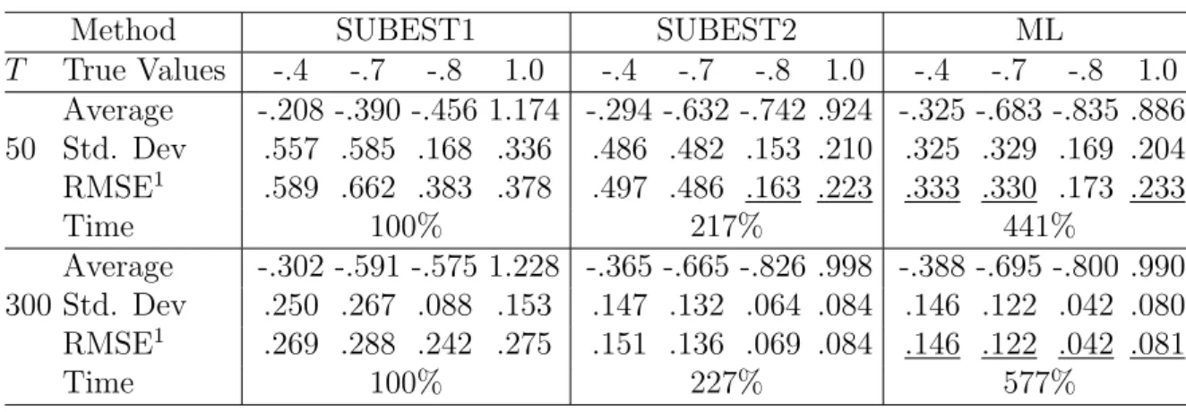
Table 4 shows the results corresponding to a gaussian ARMA(1,1)×(0,1)s
pro-cess with s = 4 and s = 12, and some redundancy between the regular AR and MA roots. Note that ML keeps the advantage in precision but its computational overhead increases the cost of SUBEST1 to 4 and 6 times in the quarterly model and 9 and 14 times in the monthly model. This is due to the increased dimension of the state vector, which also affects SUBEST2 comparative performance, and also to the degradation in conditioning, which typically requires more iterations to achieve convergence. With T = 300, ML and SUBEST2 provide very similar results in terms of accuracy.
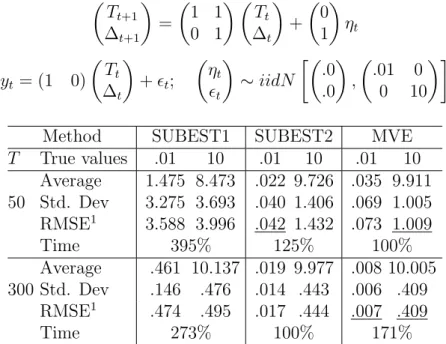
Tables 5 and 6 show the results obtained with two typical formulations in the state-space literature: an STSM with a low signal-to-noise ratio and an AR(2) model with observation errors, respectively. Note in Table 5 that SUBEST1 is the slower method and its estimates are very imprecise in comparison with those of SUBEST2 and ML. This is mainly due to the fact that the loss function conside-red in SUBEST1 does not depend on the errors covariance matrix. Therefore, its estimates do not take into account the restriction of a null covariance between the errors in the state and observation equation. The low signal-to-noise ratio makes the matter worst, as it deteriorates the identificability of the parameters. On the other hand, SUBEST2 and ML estimates are more precise, as they take into ac-count this critical independence restriction. Their computational overhead is also similar, due to the very small number of parameters to be estimated. Results pro-vided by the Table 6 are rather similar, the main difference being the improvement of SUBEST1 owing to a higher signal-to-noise ratio.
[INSERT TABLES 5-6]
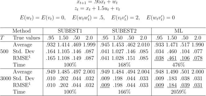
Finally, Tables 7 and 8 present results that had been obtained for two com-mon high frequency financial models: Autorregresive Stochastic Volatility (ARSV) and Generalized Autorregresive Conditional Heteroskedasticity (GARCH) Models.
Results in Table 7 are close to those of an AR model with observation errors in precision and efficiency. This was expected, because the SS representation of both models is very similar. However, when the sample size increases, the compu-tational cost of ML becomes between 5 and 20 times the cost of SUBEST1 and, between 3 and 12 times the cost of SUBEST2, for T = 500 and T = 3,000.
Table 8 shows that computational disadvantage of ML in the GARCH model is larger than in the previous case. In particular, computational load of ML becomes 49 times the cost of SUBEST1 and more than 16 times the cost of SUBEST2, for
T = 500. When the sample size increases to T = 3,000, SUBEST2 becomes the fastest method. In fact, ML converges 90 and 79 times slower than SUBEST2 and SUBEST1, respectively, while the three methods remain very similar in terms of precision.
[INSERT TABLES 7-8]
Both algorithms are very useful with high frequency financial data. Further-more, usual problems in the ML estimation of multivariate conditional heteroske-dasticity models, as convergence problems due to ill-conditioning or doubts about gaussian distribution, strongly suggest the use of these alternative estimation met-hods.
References
Anderson, B. D. O. and Moore, J. B. (1979). Optimal Filtering. Englewood Cliffs (N.J.): Prentice Hall.
Ansley, C. F. and Newbold, P. (1980). Finite sample properties of estimators for autorregresion moving average models. Journal of Econometrics, 13:159–183. Aoki, M. (1990). State Space Modelling of Time Series. Springer Verlag, New
York.
Casals, J., Sotoca, S., and Jerez, M. (1999). A fast stable method to compute the likelihood of time invariant state space models. Economics Letters, 65(3):329– 337.
Chui, N. L. C. (1997). Subspace Methods and Informative Experiments for System Identification. PhD thesis, Pembroke College Cambridge.
Dufour, J. M. and Pelletier, D. (2004). Linear estimation of weak varma models with macroeconomic applications. Technical report, Centre Interuniversitaire de Recherche en Economie Quantitative (CIREQ), Universit´e de Montr´eal, CA-NADA.
Favoreel, W., De Moor, B., and Van Overschee, P. (2000). Subspace state space system identification for industrial processes.Journal of Process Control, 10:149– 155.
Flores, R. and Serrano, G. (2002). A generalized least squares estimation method for varma models. Statistics, 36(4):303–316.
Francq, C. and Zako¨ıan, J. M. (2000). Estimating weak garch representations.
Econometric Theory, 16:692–728.
Harvey, A. C. (1989). Forecasting, structural time series models and th Kalman Filter. Cambridge University Press.
Harvey, A. C., Ruiz, E., and Shepard, N. (1994). Multivariate stochastic variance models. Review of Economic Studies, 61:247–264.
Harvey, A. C. and Shepard, N. (1993). Structural Time Series Models, volume 11 of Handbook of Statistics. Elsevier Science Publishers B.V.
Ho, B. and Kalman, R. (1966). Effective construction of linear state-variable models from input-output functions. Regelungstechnik, 14:545–548.
Koreisha, S. G. and Pukkila, T. H. (1989). Fast linear estimation methods for vector autorregresive moving average models. Journal of Time Series Analysis, 10:325–339.
Koreisha, S. G. and Pukkila, T. H. (1990). A generalized least-squares approach for estimation of autorregresive moving-average models. Journal of Time Series Analysis, 11:139–151.
Ljung, L. (1999). System Identification, Theory for the User. PTR Prentice Hall. L¨utkepohl, H. and Poskitt, D. S. (1996). Specification of echelon form varma
models. Journal of Business and Economic Statistics, 14(1):69–79.
Peternell, K., Sherrer, W., and Deistler, M. (1996). Statistical analysis of novel subspace identification methods. Signal Processing, 52:161–177.
Spliid, H. (1983). A fast estimation method for the vector autoregressive moving average model with exogenous variables. Journal of the American Statistical Association, 78(384):843–849.
Terceiro, J. (1990). Estimation of Dynamics Econometric Models with Errors in Variables. Springer-Verlag, Berlin.
Van Overschee, P. and De Moor, B. (1996). Subspace Identification for Linear Systems: Theory, Implementation, Applications. Kluwer Academic, Dordrecht, The Netherlands.
Viberg, M. (1995). Subspace-based methods for the identification of the linear time-invariant systems. Automatica, 31(12):1835–1852.
A
Appendix
From equation (10), displacing time subscripts, we obtain:
Zf+ = Oi−1Xi+1+Hd
i−1Uf++H
s
i−1Ef+ (26)
Note that Zf+ includes only the future block information whileZf integrates the
present and the future. On the other hand, from the state equation in (2), we can express: xt = (Φ−EH)ixt−i+ i−1 X j=0 (Φ−EH)j[Ezt−1−j + (Γ−ED)ut−1−j] (27)
which can be written in subspace form as,
Xi = (Φ−EH)iXp+Ψi(Φ−EH, E)Zp+Ψi(Φ−EH,Γ−ED)Up (28)
where Ψi(A, B) = [Ai−1B Ai−2B ... AB B]. Again, displacing time in-dices, we write:
Xi+1 = (Φ−EH)i+1Xp++Ψi+1(Φ−EH, E)Zp++Ψi+1(Φ−EH,Γ−ED)Up+ (29)
or, in the same way,
Finally, substituting (30) into (26), we obtain:
Zf+ =Oi−1[(Φ−EH)Xi+EZpr+ (Γ−ED)Upr] +Hid−1Uf++His−1Ef+ (31)
B
Appendix
To obtain the equations of the Kalman Filter (Anderson and Moore, 1979) in subspace form, we must propagate i times equations:
ˆ Zpr = HXˆi|i−1+DUpr (32) ˆ Xi+1|i = Φ ˆXi|i−1 + ΓUpr +Ki(Zpr −Zˆpr) (33) Ki = (ΦPi|i−1H0 +ESC0)B0i (34) Pi+1|i = ΦPi|i−1Φ0 +EQE0 −KiBiKi0 (35) Bi = HPi|i−1H0 +CRC0 (36)
From (33) we get K˜i, an approximation for Ki as,
˜ Ki = (Xˆi+1−ΓUprπU,Zp+) ˜ Zpr (37)
where the state sequence is computed as,
ˆ Xi+1=Oi+−1(Zf+πU,Z p+ −H d i−1Uf+πU,Zp+) (38) and Z˜pr as, ˜ Zpr =ZprπU,Zp −OiXˆi−H d iUprπU,Zp (39)
Finally, an approximation of Bi is obtained as,
˜
C
Appendix
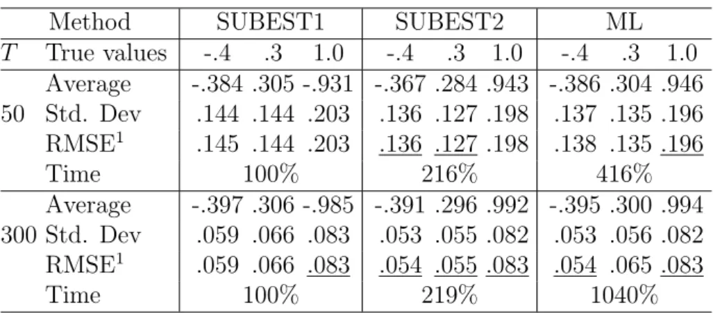
Table 1: Univariate nonseasonal models with gaussian errors.
Table 1.1 AR model (1-.4B+.3B2)Z
t=at; at ∼iidN(0,1).
Method SUBEST1 SUBEST2 ML
T True values -.4 .3 1.0 -.4 .3 1.0 -.4 .3 1.0 Average -.384 .305 -.931 -.367 .284 .943 -.386 .304 .946 50 Std. Dev .144 .144 .203 .136 .127 .198 .137 .135 .196 RMSE1 .145 .144 .203 .136 .127 .198 .138 .135 .196 Time 100% 216% 416% Average -.397 .306 -.985 -.391 .296 .992 -.395 .300 .994 300 Std. Dev .059 .066 .083 .053 .055 .082 .053 .056 .082 RMSE1 .059 .066 .083 .054 .055 .083 .054 .065 .083 Time 100% 219% 1040%
Table 1.2 ARMA model (1-.4B+.3B2)Zt = (1−.8B)at; at∼iidN(0,1).
Method SUBEST1 SUBEST2 ML
T True values -.4 .3 -.8 1.0 -.4 .3 -.8 1.0 -.4 .3 -.8 1.0 Average -.360 .289 -.671 1.020 -.307 .297 -.680 1.000 -.354 .313 -.800 .927 50 Std. Dev .305 .175 .291 .214 .222 .141 .254 .206 .196 .141 .197 .194 RMSE1 .308 .175 .318 .215 .240 .141 .281 .206 .201 .141 .197 .207 Time 100% 244% 359% Average -.398 .309 -.763 1.014 -.389 .304 -.805 1.001 -.395 .304 -.797 .993 300 Std. Dev .085 .071 .061 .085 .066 .061 .074 .083 .066 .061 .050 .081 RMSE1 .085 .072 .072 .086 .067 .062 .074 .083 .066 .062 .050 .081 Time 100% 230% 881%
1RMSE is the root mean-squared error. The smallest RMSEs are underlined. ML algorithm
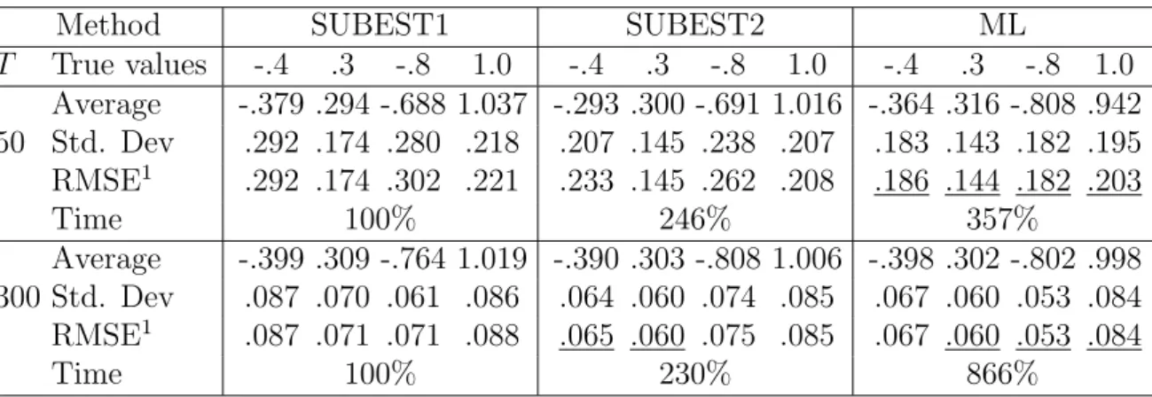
Table 2: Univariate nonseasonal models with t-student errors.
Table 2.1: ARMA model (1-.4B+.3B2)Z
t= (1−.8B)at;at∼iid t with 400 d.f.
Method SUBEST1 SUBEST2 ML
T True values -.4 .3 -.8 1.0 -.4 .3 -.8 1.0 -.4 .3 -.8 1.0 Average -.379 .294 -.688 1.037 -.293 .300 -.691 1.016 -.364 .316 -.808 .942 50 Std. Dev .292 .174 .280 .218 .207 .145 .238 .207 .183 .143 .182 .195 RMSE1 .292 .174 .302 .221 .233 .145 .262 .208 .186 .144 .182 .203 Time 100% 246% 357% Average -.399 .309 -.764 1.019 -.390 .303 -.808 1.006 -.398 .302 -.802 .998 300 Std. Dev .087 .070 .061 .086 .064 .060 .074 .085 .067 .060 .053 .084 RMSE1 .087 .071 .071 .088 .065 .060 .075 .085 .067 .060 .053 .084 Time 100% 230% 866%
Table 1.2: ARMA model (1-.4B+.3B2)Zt= (1−.8B)at; at ∼iid t with 8 d.f.
Method SUBEST1 SUBEST2 ML
T True values -.4 .3 -.8 1.3 -.4 .3 -.8 1.3 -.4 .3 -.8 1.3 Average -.383 .282 -.691 1.009 -.282 .294 -.678 .991 -.354 .308 -.802 .919 50 Std. Dev .315 .193 .314 .256 .211 .161 .255 .247 .193 .155 .207 .238 RMSE1 .315 .194 .332 .411 .242 .161 .283 .419 .199 .155 .207 .475 Time 100% 245% 368% Average -.401 .307 -.765 1.007 -.385 .302 -.808 .994 -.399 .300 -.803 .986 300 Std. Dev .088 .072 .065 .059 .066 .061 .076 .057 .068 .061 .053 .055 RMSE1 .088 .072 .074 .328 .068 .061 .077 .341 .068 .061 .053 .349 Time 100% 230% 862%
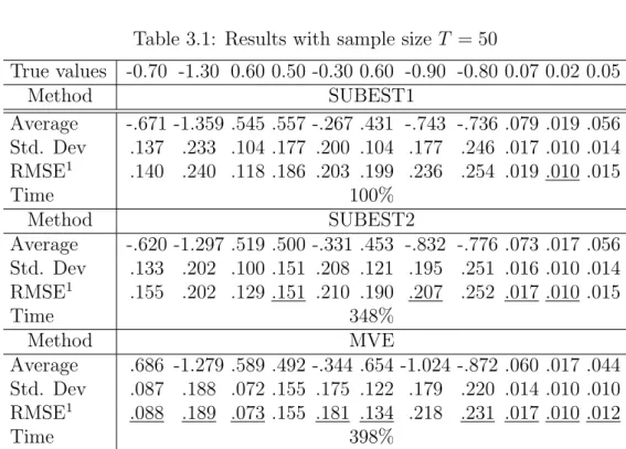
Table 3: Bivariate VARMA model with gaussian errors. 1−.7B +.6B2 0 0 1−1.3B +.5B2 z1t z2t = 1−.3B −.9B .6B 1−.8B a1t a2t a1t a2t ∼iidN .0 .0 , .07 .02 − .05
Table 3.1: Results with sample size T = 50
True values -0.70 -1.30 0.60 0.50 -0.30 0.60 -0.90 -0.80 0.07 0.02 0.05 Method SUBEST1 Average -.671 -1.359 .545 .557 -.267 .431 -.743 -.736 .079 .019 .056 Std. Dev .137 .233 .104 .177 .200 .104 .177 .246 .017 .010 .014 RMSE1 .140 .240 .118 .186 .203 .199 .236 .254 .019 .010 .015 Time 100% Method SUBEST2 Average -.620 -1.297 .519 .500 -.331 .453 -.832 -.776 .073 .017 .056 Std. Dev .133 .202 .100 .151 .208 .121 .195 .251 .016 .010 .014 RMSE1 .155 .202 .129 .151 .210 .190 .207 .252 .017 .010 .015 Time 348% Method MVE Average .686 -1.279 .589 .492 -.344 .654 -1.024 -.872 .060 .017 .044 Std. Dev .087 .188 .072 .155 .175 .122 .179 .220 .014 .010 .010 RMSE1 .088 .189 .073 .155 .181 .134 .218 .231 .017 .010 .012 Time 398%
1RMSE is the root mean-squared error. The smallest RMSEs are underlined. ML algorithm
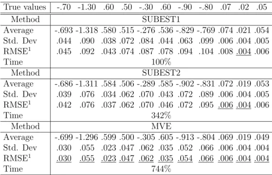
Table 3.2: Results with sample size T = 300 True values -.70 -1.30 .60 .50 -.30 .60 -.90 -.80 .07 .02 .05 Method SUBEST1 Average -.693 -1.318 .580 .515 -.276 .536 -.829 -.769 .074 .021 .054 Std. Dev .044 .090 .038 .072 .084 .044 .063 .099 .006 .004 .005 RMSE1 .045 .092 .043 .074 .087 .078 .094 .104 .008 .004 .006 Time 100% Method SUBEST2 Average -.686 -1.311 .584 .506 -.289 .585 -.902 -.831 .072 .019 .053 Std. Dev .039 .076 .034 .062 .070 .043 .072 .089 .006 .004 .005 RMSE1 .042 .076 .037 .062 .070 .046 .072 .095 .006 .004 .006 Time 342% Method MVE Average -.699 -1.296 .599 .500 -.305 .605 -.913 -.804 .069 .019 .049 Std. Dev .030 .055 .023 .047 .062 .035 .052 .066 .006 .004 .004 RMSE1 .030 .055 .023 .047 .062 .035 .054 .066 .006 .004 .004 Time 744%
Table 4: Univariate seasonal ARMA models.
Table 4.1 ARMA model (1−.4B)Zt= (1−.7B)(1−.8B4)at; at∼iidN(0,1.0)
Method SUBEST1 SUBEST2 ML
T True Values -.4 -.7 -.8 1.0 -.4 -.7 -.8 1.0 -.4 -.7 -.8 1.0 Average -.208 -.390 -.456 1.174 -.294 -.632 -.742 .924 -.325 -.683 -.835 .886 50 Std. Dev .557 .585 .168 .336 .486 .482 .153 .210 .325 .329 .169 .204 RMSE1 .589 .662 .383 .378 .497 .486 .163 .223 .333 .330 .173 .233 Time 100% 217% 441% Average -.302 -.591 -.575 1.228 -.365 -.665 -.826 .998 -.388 -.695 -.800 .990 300 Std. Dev .250 .267 .088 .153 .147 .132 .064 .084 .146 .122 .042 .080 RMSE1 .269 .288 .242 .275 .151 .136 .069 .084 .146 .122 .042 .081 Time 100% 227% 577%
Table 4.2 ARMA model (1−.4B)Zt= (1−.7B)(1−.8B12)at; at ∼iidN(0,1.0)
Method SUBEST1 SUBEST2 ML
T True values -.4 -.7 -.8 1.0 -.4 -.7 -.8 1.0 -.4 -.7 -.8 1.0 Average -.240 -.493 -.368 1.133 -.244 -.592 -.494 1.073 -.324 -.680 -.807 .902 50 Std. Dev .525 .534 .128 .261 .438 .454 .042 .237 .331 .323 .224 .225 RMSE1 .549 .572 .450 .293 .465 .467 .309 .248 .340 .323 .224 .245 Time 100% 436% 907% Average -.374 -.661 -.586 1.221 -.379 -.691 -.812 .970 -.386 -.694 -.805 .984 300 Std. Dev .221 .201 .055 .118 .143 .128 .073 .084 .135 .112 .048 .083 RMSE1 .222 .205 .221 .250 .145 .128 .074 .089 .136 .112 .048 .085 Time 100% 371% 1415%
1RMSE is the root mean-squared error. The smallest RMSEs are underlined. ML algorithm
Table 5: Structural time series model. Tt+1 ∆t+1 = 1 1 0 1 Tt ∆t + 0 1 ηt yt = (1 0) Tt ∆t +t; ηt t ∼iidN .0 .0 , .01 0 0 10
Method SUBEST1 SUBEST2 MVE
T True values .01 10 .01 10 .01 10 Average 1.475 8.473 .022 9.726 .035 9.911 50 Std. Dev 3.275 3.693 .040 1.406 .069 1.005 RMSE1 3.588 3.996 .042 1.432 .073 1.009 Time 395% 125% 100% Average .461 10.137 .019 9.977 .008 10.005 300 Std. Dev .146 .476 .014 .443 .006 .409 RMSE1 .474 .495 .017 .444 .007 .409 Time 273% 100% 171%
Table 6: AR model with observation errors.
(1−1.5B+.8B2)z∗ t =at; zt=zt∗+vt; at vt ∼iidN .0 .0 , 1.0 0 0 .5
Method SUBEST1 SUBEST2 ML
T True values -1.5 .8 1.0 .5 -1.5 .8 1.0 .5 -1.5 .8 1.0 .5 Average -1.425 .731 1.030 .558 -1.429 .737 1.045 .558 -1.480 .781 .954 .469 50 Std. Dev .268 .187 .219 .202 .133 .121 .195 .177 .128 .119 .185 .169 RMSE1 .278 .199 .221 .210 .150 .136 .200 .186 .129 .121 .190 .172 Time 100% 204% 142% Average -1.491 .798 .990 .530 -1.487 .788 1.010 .513 -1.492 .793 .997 .493 300 Std. Dev .057 .046 .081 .069 .047 .044 .075 .057 .044 .043 .072 .055 RMSE1 .057 .047 .081 .076 .048 .046 .076 .059 .045 .043 .072 .056 Time 100% 193% 253%
Table 7: ARSV(1) model in State Space form.
xt+1 =.95xt+wt
zt=xt+ 1.5ut+vt
E(wt) =E(vt) = 0, E(wtw0t) = .5, E(vtvt0) = 2, E(wtvt0) = 0
Method SUBEST1 SUBEST2 ML
T True values .95 1.50 .50 2.0 .95 1.50 .50 2.0 .95 1.50 .50 2.0 Average .932 1.414 .469 1.999 .945 1.453 .462 2.010 .933 1.471 .517 1.990 500 Std. Dev .164 1.105 .146 .087 .041 1.027 .146 .085 .034 .460 .104 .077 RMSE1 .165 1.108 .149 .087 .041 1.028 .151 .085 .038 .461 .106 .078 Time 100% 168% 476% Average .949 1.485 .497 2.001 .949 1.484 .494 2.004 .948 1.490 .501 2.000 3000 Std. Dev .010 .202 .044 .032 .009 .198 .044 .033 .009 .183 .038 .031 RMSE1 .010 .202 .044 .032 .009 .198 .044 .033 .009 .184 .039 .031 Time 100% 166% 2059%
Table 8: GARCH(1,1) model in ARMA form.
yt=t with t ∼iid(0,1.0) andt|Ωt−1 ∼iidN(0, σt2) where
t2 = 1.0 + 11−−..9780BBvt with vt=2t −σ2t
Method SUBEST1 SUBEST2 ML
T True values 1.0 -.97 -.80 1.0 -.97 -.80 1.0 -.97 -.80 Average 1.005 -.972 -.798 1.002 -.969 -.814 1.209 -.952 -.784 500 Std. Dev .766 .025 .076 .760 .031 .106 1.420 .037 .056 RMSE1 .766 .025 .076 .760 .031 .107 1.436 .041 .058 Time 100% 298% 4916% Average .999 -.974 -.810 .998 -.972 -.809 1.095 -.967 -.797 3000 Std. Dev .314 .015 .052 .313 .019 .068 .880 .011 .018 RMSE1 .314 .016 .053 .313 .019 .069 .885 .011 .018 Time 114% 100% 9047%
1RMSE is the root mean-squared error. The smallest RMSEs are underlined. ML algorithm