Rochester Institute of Technology Rochester Institute of Technology
RIT Scholar Works
RIT Scholar Works
Theses
10-2019
Vector Spaces for Multiple Modal Embeddings
Vector Spaces for Multiple Modal Embeddings
Sabarish GopalakrishnanFollow this and additional works at: https://scholarworks.rit.edu/theses
Recommended Citation Recommended Citation
Gopalakrishnan, Sabarish, "Vector Spaces for Multiple Modal Embeddings" (2019). Thesis. Rochester Institute of Technology. Accessed from
This Thesis is brought to you for free and open access by RIT Scholar Works. It has been accepted for inclusion in Theses by an authorized administrator of RIT Scholar Works. For more information, please contact
Vector Spaces for Multiple Modal Embeddings
BySabarish Gopalakrishnan
October 2019 A Thesis Submitted in Partial Fulfillmentof the Requirements for the Degree of Master of Science
in
Computer Engineering
Committee Approval:
Dr. Raymond Ptucha, Advisor Date
Associate Professor
Dr. Alexander Loui, Committee Member Date
Professor
Dr. Qi Yu, Committee Member Date
Associate Professor
2 | P a g e
Acknowledgments
I would like to take this opportunity to thank my advisor Dr. Raymond Ptucha for his continual support and guidance during my master’s degree. I am thankful for Dr. Alexander Loui and Dr. Qi Yu for being in my thesis committee. I would like to give a personal thank you to Dr. Shagan Sah for being a mentor and guiding force throughout my master’s. I would also like to thank my family and my close friends, without their support this journey would not have been as joyful as it was.
3 | P a g e
Abstract
Deep learning has enabled great advances in the field of natural language processing, computer vision and pattern recognition in general. Deep learning frameworks have been very successful in performing classification, object detection, segmentation and translation. Before objects can be processed, a vector representation of that object needs to be created. For example, sentences and images can be encoded with a sent2vec and image2vec function respectively in preparation for input to a machine learning framework. Neural networks are able to learn efficient vector representation of images, text, audio, videos and 3D point clouds. However, the transfer of knowledge from one modality to the other is a challenging task. In this work, we develop vector spaces that can handle data that belongs to multiple modalities at the same time. In these spaces, similar objects are tightly clustered and dissimilar objects are far away irrespective of their modality. Such a vector space can be used in retrieval of objects, searching and generation tasks. For example, given a picture of a person surfing, one can retrieve sentences or audio bites of a person surfing. We build a Multi-stage Common Vector Space (M-CVS) and Reference Vector Space (RVS) that can handle images, text, audios, videos and 3D point cloud data. Both, the M-CVS and RVS can handle the addition of a new modality without having to change the existing transforms or architecture. Our model is evaluated by performing cross modal retrieval on multiple benchmark datasets.
4 | P a g e
Contents
Vector Spaces for Multiple Modal Embeddings ... 1
List of Figures ... 6 List of Tables ... 8 Chapter 1 ... 9 1.1 Introduction ... 9 1.2 Motivation ... 10 1.3 Contributions ... 11 Chapter 2 ... 12 2.1 Deep Learning ... 12
2.2 Convolutional Neural Networks ... 12
2.3 Recurrent Neural Networks ... 14
A. Long Short Term Memory (LSTM) ... 16
B. Gated Recurrent United (GRU) ... 17
2.4 Multi-modal and Cross-modal Retrieval ... 18
2.5 Metric Learning Loss Functions ... 21
A. Contrastive Loss Function [38] ... 21
B. Triplet Loss Function [12] ... 21
C. Adversarial Loss Function [57]... 22
2.6 Semi-Hard Negative Mining ... 23
Chapter 3 ... 24
3.1 Common Vector Space (CVS) ... 25
A. Loss Functions ... 27
B. Training Strategy ... 29
C. Aligned Attention ... 30
D. Limitations of the CVS Model ... 32
3.2 Multi-Staged Common Vector Space (M-CVS) ... 32
A. Training Strategy ... 33
3.3 Reference Vector Space (RVS) ... 34
A. Aligned Attention for RVS ... 35
3.4 Stage Wise Learning for Multi Modal Embeddings ... 37
A. Training Strategy ... 38
5 | P a g e
4.1 Datasets ... 39
A. XMedia [11, 47] and XMediaNet [51,59] ... 39
B. Nuswide [49] and Pascal [50] ... 42
C. Birds [58] ... 42
4.2 Implementation ... 43
A. Evaluation Metric ... 43
B. Intuitive Understanding of mAP ... 44
Chapter 5 ... 46
5.1 Results ... 46
A. CVS Model: Pascal and Nuswide ... 46
B. CVS Model: XMedia and XMediaNet (2 modalities) ... 47
C. CVS Model: Xmedia and XMediaNet (5 modalities) ... 47
D. M-CVS Model: Xmedia and XMediaNet (5 modalities) ... 49
E. RVS Model: Xmedia and XMediaNet (5 modalities) ... 50
F. Stagewise Learning ... 52
5.2 Ablation Analysis ... 53
A. Attention Ablation Analysis... 53
B. Timing Analysis ... 55
C. Adversarial Loss Functions ... 55
Chapter 6 ... 57
6.1 Conclusions ... 57
6.2 Discussions ... 57
6.3 Future Work ... 58
6 | P a g e
List of Figures
Figure 1: Typical CNN architecture. An image passes through multiple convolutions and filtering operations before being passed through fully connected layers and classified into a one out of several
classes. ... 13
Figure 2: Convolution Operation. Left – Input array; right – convolution kernel. ... 13
Figure 3: Max poling operation in a convolutional neural network. ... 14
Figure 4: A recurrent neural network consisting of many sequential cells that take input from the previous state and also the current input to predict the output at each time step. ... 15
Figure 5: LSTM cell with input, output and forget cells that allows it to retain important information. ... 16
Figure 6: A GRU unit which has comparatively fewer parameters and is easier to train and tune. ... 17
Figure 7: The DSCMR [43] architecture consisting of three sepearate loss functions to perform cross modal retrieval. ... 20
Figure 8 Cases for the triplet loss. Loss is only updated in the bottom two cases when the negative is closer to the positive and the anchor. ... 22
Figure 9: The vector space before (left) and after (right) training. The colors represent the different data modalities and the shapes represent the categories. ... 24
Figure 10 Architecture for the CVS model. Data belonging to different modalities will get encoded into vectors after which they are projected into the common embedding space using fully connected layers. . 26
Figure 11 Cosine distance between two vectors in a 2D representation. ... 27
Figure 12: The adversarial loss function is calculated by comparing the generated and input images and sentences. ... 28
Figure 13 Aligned attention block which takes in two inputs and gives two corresponding outputs. ... 32
Figure 14 Architecture for the Multi-Stage CVS Model. Every additional stage takes n new attention blocks. ... 34
Figure 15 Architecture for the RVS model which has 1 attention block for every data modality present in the RVS. ... 35
Figure 16 Attention mechanism for the RVS model. ... 36
Figure 17: Step by step implementation of stage-wise learning. ... 38
Figure 18: Example from the XMedia [11, 47] dataset. ... 40
Figure 19 Example from the XMediaNet [51, 59] dataset. ... 41
Figure 20: Sample images from the Nuswide dataset. [49] ... 42
Figure 21: A visualization of mean average precision. ... 44
Figure 22 The total loss for the CVS model as a function of the epochs visualized on Tensorboard. ... 48
Figure 23: The metric loss for the M-CVS model with respect to the total epochs. ... 50
Figure 24: The decrease in the cross entropy loss with respect to the total number of epochs in the RVS model. ... 51
Figure 25 Effect of all the 3 components of attention. ... 54
7 | P a g e Figure 27: The time per iteration for the CVS and the M-CVS model as we increase the number of
modalities added to the model. ... 55 Figure 28: Non converging of the reconstruction loss for the image and text modality. ... 56
8 | P a g e
List of Tables
Table 1: XMedia and XMediaNet dataset statistics. Figures indicate the number of training and testing
samples. ... 41
Table 2: XMedia and XMediaNet Features and their dimensions. ... 42
Table 3: Pascal and Nuswide dataset statistics. Figures indicate the train and test splits. ... 43
Table 4: Train and test split for the Birds dataset used to perform zero-shot retrieval. ... 43
Table 5: mAP scores for the Pascal and Nuswide dataset. ... 46
Table 6: mAP scores for the Xmedia and XMediaNet dataset. ... 47
Table 7: mAP scores for the images, text, and video for the XMediaNet dataset. ... 47
Table 8: Cross modal retrieval scores (mAP) for the five modalities in the XMedia dataset. ... 48
Table 9: Cross modal retrieval scores(mAP) for the M-CVS model on the XMedia datadset. ... 49
Table 10: mAP scores for images, text, and video for XMediaNet dataset. ... 50
Table 11: Cross modal retrieval mAP scores for the XMedia dataset. ... 51
Table 12: Stage wise learning methodology for the Pascal and Birds dataset. ... 52
9 | P a g e
Chapter 1
Introduction
1.1
Introduction
Deep learning has shown great ability to perform targeted tasks like image classification, segmentation, object detection, and language translation. With the extensive availability of data and increased understanding of loss functions, neural networks are able to generate a good understanding of images, text, audio signals and videos. Convolutional Neural Networks (CNNs) have become the default model for computer vision tasks that were traditionally done using handcrafted features. CNNs architectures are now used for image classification, image segmentation, and object detection. Further, CNNs can be used as an image encoder, compressing a very high dimensional image into a small dimensional vector. Recurrent Neural Networks (RNNs) such as Long Short Term Memory (LSTMs) have proven to perform well in sequential tasks like language translation and caption generation. Within the past few years, Generative Adversarial Networks (GANs) have been shown to generate realistic-looking images from input noise vectors. The unique selling point of all these deep learning architectures is that they are able to learn the necessary parameters to accomplish real-world tasks. These deep architectures along with their learned parameters have been shown do a better job of most tasks when compared to the traditional machine learning methods paired with handcrafted features. Often, the deep architectures are able to develop a deeper understanding of the data which may not be easily perceptible to a human being.
These deep neural networks have shown incredible ability in targeted tasks in uni-modal settings like image classification or sentence to sentence translation. However, converting from one modality to another still remains a challenge. The work by Wu et al. [27] and Huang and Peng [26] show the ability to transfer from the image to text domain while [28] shows how we can transfer from audio to video domain. Vendrov et al. [24] and You et al.
[25] show how images and text can be retrieved at the instance level whereas the works in [20, 21, 22, 23] show category level retrieval on images and text. Qi et al. [8] and Qi and Peng [10] showed cross modal retrieval using different learning techniques. Srivastava et al.
10 | P a g e
More recently, adversarial loss functions and self-supervised learning techniques have been successfully shown to perform retrieval.
1.2
Motivation
Any data processed or stored by a computer ultimately needs to be converted into a binary format. These binary numbers are the most basic representations of data for computers. Similarly, vectors are the most basic structures of objects or concepts for machine learning models. Vectors are nothing but a list of numbers on which operations could be performed. These vectors will be used as the input and outputs to the deep neural networks used in this research.
Data originating from any modality (image, text, video, etc.) is first and foremost converted to a vector representation before being fed to a deep neural network. It is therefore very important that these vector representations of data are robust and are able to relay as much information about the input data as possible. Even if a model architecture is highly optimized and robust, unless the input data vectors are efficient, the model may end up failing.
This work aims to form efficient vector representations not only for a unimodal setting but also a multimodal setting where data belonging to different modalities can seamlessly interact with each other. The transfer of knowledge from one modality to the other is done through the medium of this common embedding space that we define.
We develop an architecture that is able to handle any number of modalities, and experiments will be conducted with up to five modalities. This work describes multiple ways in which a multimodal system can be built and provides a way of mapping new modalities into the model without having to change existing transformations and inferences. This work also compares different ways to formulate such a network and develops an understanding of the various pitfalls that these models face.
Such a model can be used for remote sensing applications where a vast range of sensors pick up data in different modalities to perform tasks like object detection and activity recognition. For example, a satellite can scan the ground and pick up passive signals like RGB images, infrared images, hyperspectral images as well as active signals like LIDAR point clouds,
Synthetic-aperture radar (SAR) images etc. Similarly, sensors on the ground can pick up other information about the environment. Our model can then be used to help transfer contextual information from one modality to the other. Our model can also help in providing redundancy in
11 | P a g e case of failure of any of the modalities. Similarly, such a model proves useful in mapping medical imagery data from sources like X-Rays, MRIs, CT Scans, ultrasounds etc.
The models we develop can be further used to train a network that takes in an input from one modality and generates synthetic data in a different modality. Such generation of data can prove to be helpful in under sampled modalities.
1.3
Contributions
The main contributions of this thesis work can be summarized as:
Extend the Common Vector Space (CVS) framework into two new architectures- the Multi-stage Common Vector Space (M-CVS) and the Reference Vector Space RVS and compare the three networks.
Implement stage wise training of neural networks to see effect on performance of retrieval.
Achieve robust transfer of information across multiple modalities using the same network architecture.
12 | P a g e
Chapter 2
Background
2.1
Deep Learning
Deep learning is a branch of machine learning that deals with artificial neural networks which contain many weights or parameters, and often many hidden or intermediate layers. Deep learning works best when vast amounts of data and computing resources are available. It has provided massive breakthroughs in the fields of computer vision and language modeling. Deep learning architectures have a significant advantage over traditional methods that involve handcrafted features because the features are learned by the architecture. Additionally, the formulation of smarter loss functions has meant that deep learning can be used for a variety of tasks like image segmentation, object detection, and language translation.
2.2
Convolutional Neural Networks
Convolutional neural networks (CNNs) form the backbone of modern computer vision processing and have helped advance the field of image processing. CNNs are able to effectively extract and learn features from gridded data structures like images or video frames. The evolution of CNNs from VGG-Net [2] to more complex architectures like the Inception [5] and ResNet [6] have helped achieve state-of-the-art results on multiple benchmark datasets like the CIFAR10 [7] and ImageNet [17]. CNNs perform very well in image classification [2, 18, 6, 19], image segmentation [4], and object detection [3].
CNNs generally consist of three basic operations: convolution, pooling, and fully connected layers. The convolution layers use filter kernels to perform convolution operations on the input before passing it on to the next layer. The pooling layers down sample the input that it receives whereas the fully connected layers form multi-layer perceptron layers to finally arrive at the sample classification. At a high level, the convolution and pooling layers extract a salient hierarchy of features, and the fully connected layers perform the classification. One reason this architecture is so powerful is that both the features and classifier components are learned simultaneously through a process called backpropagation.
13 | P a g e
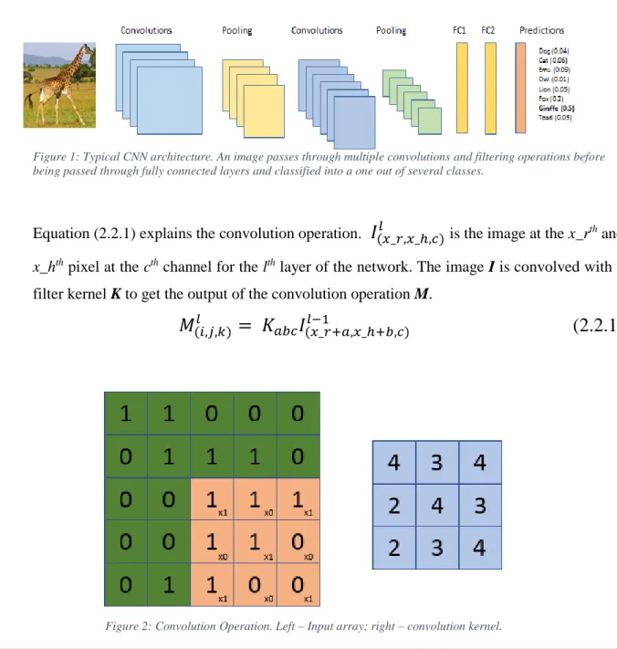
The convolution operation typically preserves the output dimensions of the input provided necessary padding of the original input is done. On the other hand, pooling decreases the dimensions of the data. Average pooling and max-pooling are the two most popularly used pooling techniques. Figure 1 shows a typical CNN architecture for an image classification setting. An input image passes through various convolution and pooling layers. Finally, it is flattened out to form a single vector. This single vector is then passed through multiple fully connected layers after which a final layer performs classification. The connections between layers use non-linear activation functions like the sigmoid, tanh and relu so that the network can learn some very complex patterns.
Figure 1: Typical CNN architecture. An image passes through multiple convolutions and filtering operations before being passed through fully connected layers and classified into a one out of several classes.
Equation (2.2.1) explains the convolution operation.
𝐼
(𝑥_𝑟,𝑥_ℎ,𝑐)𝑙 is the image at the x_rth andx_hth pixel at the cthchannel for the lth layer of the network. The image I is convolved with a filter kernel K to get the output of the convolution operation M.
𝑀
(𝑖,𝑗,𝑘)𝑙= 𝐾
𝑎𝑏𝑐𝐼
(𝑥_𝑟+𝑎,𝑥_ℎ+𝑏,𝑐)𝑙−1(2.2.1)
14 | P a g e
In Figure 2, the input array (image) is convolved with the filter to form a new output array. This filter is a matrix of parameters that are learned during backpropagation in a CNN. The learning of many such filters along with the fully connected layers enable the CNN to learn abstract concepts.
Figure 3: Max poling operation in a convolutional neural network.
Figure 3 shows a max-pooling operation where the maximum value of the cells belonging to the same color is passed to the next layer.
Videos are essentially a sequence of images and hence, CNNs are useful for encoding videos too. Karpathy et al. [31] showed an efficient way to encode videos into their vector representations. Recent works like [32, 33] show different ways in which videos can be encoded into a vector representation for tasks such as classification or segmentation.
2.3
Recurrent Neural Networks
Recurrent Neural Networks (RNNs) along with Long Short Term Memory (LSTMs) units and Gated Recurrent Units (GRUs) help encode and decode sequential data. These RNNs have the ability to retain important information in the sequence. They are used extensively to represent textual data. RNNs are used in tasks like image captioning and sentence encoding.
15 | P a g e
Work in natural language processing has led to the development of architectures that are able to perform tasks like image captioning [14 15] and video summarization [16]. Kiros et al. [13] showed how sentences can be encoded into vectors.
Figure 4: A recurrent neural network consisting of many sequential cells that take input from the previous state and also the current input to predict the output at each time step.
In the Figure 4, x1, x2…xtare the inputs for time step t = 1 to t and y1, y2…yt is the predicted
next outputs.
ℎ
𝑡= 𝑓(𝑊
ℎℎℎ
𝑡−1+ 𝑊
ℎ𝑥𝑥
𝑡)
(2.3.1)
𝑦
𝑡= 𝑠𝑜𝑓𝑡𝑚𝑎𝑥(𝑊
𝑆ℎ
𝑡)
(2.3.2)
𝐽
(𝑡)(𝜃) = ∑( 𝑦
𝑡𝑖𝑙𝑜𝑔𝑦
𝑡𝑖)
(2.3.3)
The above equations describe the working of the RNNs. The information about the previous time steps is held in (2.3.1) where ht is calculated based on ht-1. h0 is set to a vector of zeros. A
sigmoid activation is then applied to the final summation as seen in (2.3.2). In (2.3.3), the loss is calculated at each time step to find out the error between the input word and the predicted word.
16 | P a g e
RNNs face the problems of vanishing gradients and hence LSTMs and GRUs have become the default way to model sequential data.
A.
Long Short Term Memory (LSTM)
The vanishing gradient problem with RNNs is overcome using LSTMs and GRUs. LSTMs are able to selectively remember both long and short-term information. They were introduced in [34] which outperformed vanilla RNNs.
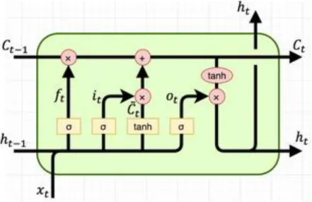
Figure 5: LSTM cell with input, output and forget cells that allows it to retain important information. [62]
𝑖
𝑡= 𝜎(𝑥
𝑡𝑈
𝑖+ ℎ
𝑡−1𝑊
𝑖)
(2.3.4)
𝑓
𝑡= 𝜎(𝑥
𝑡𝑈
𝑓+ ℎ
𝑡−1𝑊
𝑓)
(2.3.5)
𝑜
𝑡= 𝜎(𝑥
𝑡𝑈
𝑜+ ℎ
𝑡−1𝑊
𝑜)
(2.3.6)
Ć
𝑡= 𝑡𝑎𝑛ℎ(𝑥
𝑡𝑈
𝑔+ ℎ
𝑡−1𝑊
𝑔)
(2.3.7)
𝐶
𝑡= 𝜎(𝑓
𝑡∗ 𝐶
𝑡−1+ 𝑖
𝑡∗ Ć
𝑡)
(2.3.8)
17 | P a g e
ℎ
𝑡= 𝑡𝑎𝑛ℎ(𝐶
𝑡) ∗ 𝑜
𝑡(2.3.9)
Equations (2.3.3) – (2.3.9) describe the mathematics of the LSTM cell. Figure 5 shows the internal diagram of the LSTM cell. Here, I, f, o shown indicate input, forget and output gates respectively. W indicates the recurrent connection from the previous hidden state and the U is the weight matrix that transforms the inputs to the current hidden layer. The sigmoid function converts all the values to (0, 1) and helps define the information that can flow through the gates.
Ć
𝑡 is the hidden state while C is the internal memory unit. This memory unit helps to combine the current inputs and context from the previous hidden states to generate a better vector representation of the input. It is this vector representation that we generally use to encode our text data.B.
Gated Recurrent United (GRU)
GRUs is a variant of LSTMs which have fewer parameters and easier to train on. It was introduced by Cho et al. [35]. Figure 6 shows the structure of a GRU.
Figure 6: A GRU unit which has comparatively fewer parameters and is easier to train and tune. [62]
𝑧
𝑡= 𝜎(𝑥
𝑡𝑈
𝑧+ ℎ
𝑡−1
𝑊
𝑧)
(2.3.10)
𝑟
𝑡= 𝜎(𝑥
𝑡𝑈
𝑟+ ℎ
18 | P a g e
ĥ
𝑡= 𝑡𝑎𝑛ℎ(𝑥
𝑡𝑈
ℎ+ (𝑟
𝑡
∗ ℎ
𝑡−1)𝑊
ℎ)
(2.3.12)
ℎ
𝑡= (1 − 𝑧
𝑡) ∗ ℎ
𝑡−1+ 𝑧
𝑡∗ ĥ
𝑡)
(2.3.13)
Equations (2.3.10) – (2.3.13) describe the mathematical operation of the GRUs. The r is the reset gate while z is the update gate. The reset gate measures how much of the new input will be combined with the memory and the update gate defines how much of the previous memory will be kept. Assigning reset to 1 and update to 0, we have the original RNN model.
2.4
Multi-modal and Cross-modal Retrieval
Cross-modal retrieval has gained significant traction in the last decade due to the availability of vast amounts of data. The information retrieval from one modality to another is a challenging task because of the difference in their statistical properties. Most traditional techniques involve the formulation of a latent space in which the properties of the two modalities can be matched. Canonical Correlation Analysis (CCA) [53] is one technique that learns to maximize the correlation of the data belonging to different modalities.
More recently, with the development of deep learning techniques, the field of cross-modal retrieval has seen tremendous development. Deep learning has helped improve the way in which data can be encoded into vectors. Similarly, models have been built that have transferred knowledge across multiple modalities. Most work in the multi-modal space restricts itself to only two modalities. There are two types of works in the modal retrieval space: 1) cross-modal hashing [36, 37] which maps the data into a common space in a computationally efficient manner which would make retrieval faster; and 2) real-value based cross-modal retrieval which uses different loss functions to perform retrieval.
Zhang et al. [60] developed a framework that generated vector representations of sentences while Sah et al. [61] used multiple captions to generate images from common vector representations. Deng et al. [45] performed cross-modal hashing using a triplet based hashing network and Wu et al. [46] showed the use of adversarial training by using cycle consistency loss function. The task of real-value based retrieval can be modeled in different ways. Qi et al.
19 | P a g e
a model whose objective function ensured that the encoded vector representation of anchors and their corresponding positive samples lie close in the latent space, while the encoded vector representation anchors and negative samples are pushed far away. Feng et al. [22] used correspondence auto encoders while Qi and Peng [9] used reinforcement learning to perform cross-modal retrieval.
Zhen et al. [43] used a combination of a modality invariance loss, linear classifier, intermodal and intramodal discriminative loss to perform retrieval as shown in (2.4.1) and (2.4.2) and (2.4.6) respectively. Figure 7 shows the architecture used by the DSCMR [43] model. The image and text are passed through separate CNNs and their feature vectors are extracted. The losses described in (2.4.1), (2.4.2) and (2.4.6) are then calculated on these common space vectors.
𝐿
𝑖𝑛𝑣=
𝑁1||𝑈 − 𝑉||
𝐹(2.4.1)
𝐿
𝑐𝑙𝑎𝑠𝑠=
𝑁1||𝑃
𝑇𝑈 − 𝑌||
𝐹+
𝑁1||𝑃
𝑇𝑉 − 𝑌||
𝐹(2.4.2)
𝐿
𝑖𝑛𝑡𝑒𝑟=
1 𝑁2∑
(log (1 + 𝑒
Ѓ𝑖𝑗) − 𝑆
𝑖𝑗𝛼𝛽Ѓ
𝑖𝑗)
𝑁 𝑖,𝑗=1(2.4.3)
𝐿
𝑖𝑚𝑔=
𝑁12∑
(log (1 + 𝑒
Ф𝑖𝑗) − 𝑆
𝑖𝑗𝛼𝛼Ф
𝑖𝑗)
𝑁 𝑖,𝑗=1(2.4.4)
𝐿
𝑡𝑥𝑡=
1 𝑁2∑
(log (1 + 𝑒
𝜃𝑖𝑗) − 𝑆
𝑖𝑗𝛽𝛽𝜃
𝑖𝑗)
𝑁 𝑖,𝑗=1(2.4.5)
𝐿
𝑚𝑜𝑑𝑎𝑙= 𝐿
𝑖𝑛𝑡𝑒𝑟+ 𝐿
𝑖𝑚𝑔+ 𝐿
𝑡𝑒𝑥𝑡(
2.4.6)
Where:20 | P a g e
Ф
𝑖𝑗 is the cosine distance between two data points belonging to image modality.
𝜃
𝑖𝑗 is the cosine distance between two data points belonging to text modality.
𝑆
𝑖𝑗𝛼𝛼, 𝑆
𝑖𝑗𝛼𝛽, 𝑆
𝑖𝑗𝛽𝛽 are indicator functions whose value is 1 if the two elements are of same class and 0 otherwise.Figure 7: The DSCMR [43] architecture consisting of three sepearate loss functions to perform cross modal retrieval.
Xu et al. [42] used adversarial loss functions and built an architecture that converted a 4096-dimensional vector representation to a 200 dimension vector using fully connected layers. Peng
et al. [47] created an architecture that was able to retrieve images from their outline sketches and vice-versa. Works in [55, 56] show the use of retrieval of data from one modality to the other at the granular level where the input query is able to retrieve its corresponding ground-truth sample of the other modality.
Many image captioning works like [39, 40] use attention mechanism to better align words and image regions. Similarly, the attention mechanism proposed by Lee et al. [41] can be used for a better correlation between vectors belonging to different modalities. Attention models provide important context to different parts of the input text and the different regions of the image. This idea can be extended to other modalities as well if attention is applied to multi-dimensional feature vector that is formed after the encoding network.
In our work, we focus on the CUB-Birds [58], Pascal [50], NUSWIDE [49] datasets have data belonging to two modalities and also extend the ability of our model to handle up to five modalities where we test our model on the XMedia [47, 48] and XMediaNet [51, 59] datasets.
21 | P a g e
2.5
Metric Learning Loss Functions
The backbone of all deep learning applications is to define an appropriate loss function for the required task. Metric learning is a type of learning that is able to map similar representations of data between two or more modalities. Metric learning involves the process of formulating pairs of positive and negative data to achieve the required alignment in the data. The following are some of the popular metric learning loss functions that have been developed.
A.
Contrastive Loss Function [38]
Introduced by Hadsell et al. [38], the contrastive loss function calculates the distance between the encoding of the image and the text data points. The goal of the loss function is to have the negative pairs at least a distance of margin away from the positive pairs where the distance calculated is the Euclidian distance between two points.
𝐿𝑐 =
12𝑁
∑((𝑦)𝑑
2
+ (1 − 𝑦) 𝑚𝑎𝑥(𝑚𝑎𝑟𝑔𝑖𝑛 − 𝑑, 0)
2)
(2.5.1)
Where
d is the distance between image and sentence pair
y is 1 if the two samples are similar and 0 if they are dissimilar.
B.
Triplet Loss Function [12]
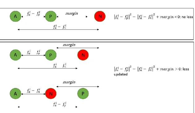
The triplet loss function forms triplets of data instead of pairs that are formed by the contrastive loss. Schroff et al. [12] developed this loss where an anchor, positive and a negative sample is selected. The objective of the loss function is to minimize the distance between the anchor and the positive sample while keeping the distance between the anchor and negative sample at least a margin apart, where the margin is similar to that used in the contrastive loss. The distance function used in the triplet loss is the Euclidian distance. Figure 8 depicts the different circumstances when the triplet loss will be updated.
𝐿
𝑇=
12𝑁
∑ 𝑚𝑎𝑥(0, |𝑓
𝑎 𝑖− 𝑓
22 | P a g e
Where
faiis the feature embedding of the anchor
fpi is the feature embedding of the positive sample fni is the feature embedding of the negative sample
Figure 8 Cases for the triplet loss. Loss is only updated in the bottom two cases when the negative is closer to the positive and the anchor.
C.
Adversarial Loss Function [57]
Adversarial loss functions have been successfully able to generate images from noise vectors using discriminator and generator networks. There are two goals of adversarial training: 1) to train a discriminator network that is unable to distinguish between real and fake data, and 2) train a generator network that can seamlessly generate fake samples of data that will be able to fool the discriminator.
(𝑚𝑖𝑛 𝐺, 𝑚𝑎𝑥 𝐷) 𝐿(𝐷, 𝐺) = 𝐸𝑥~𝑝𝑑𝑎𝑡𝑎(𝑥)[𝑙𝑜𝑔 𝐷(𝑥)] + 𝐸𝑥~𝑝𝑧(𝑧)[𝑙𝑜𝑔 (1 − 𝐷(𝐺(𝑧)))]
(2.5.3)
Where
23 | P a g e 𝐺 – Generator whose goal is to build a network that is very good at fooling the
discriminator
x, z – real and generated samples
2.6
Semi-Hard Negative Mining
In practice, it is easy to find pairs of positive and negative samples that are a margin distance apart. Since these pairs already satisfy the underlying condition, they will not contribute to the loss calculation. Semi-hard negative mining used by Schroff [12] et al. is a technique where the harder of the negative samples are used to calculate the loss and allow for better and faster convergence of the network.
The negative samples can be categorized as below:
hard – they are closer to the anchor than positive samples
Semi-hard – they lie within margin distance from the positive samples
easy negatives – they lie beyond the positive samples
The selection of easy negatives results in a loss value of zero whereas the selection of hard negatives results in a loss value that could be too high for the model to handle. Therefore, the semi-hard negatives are just the right negative samples that can help our model converge.
24 | P a g e
Chapter 3
Methodology
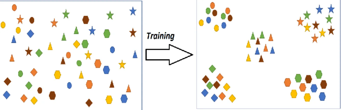
In this section, we introduce the various architectures and networks that will be used in this research and explore the differences between them. Figure 8 describes an ideal transformation that will happen with a common vector representation. Initially, when the model is randomly initialized, we see that all the points in the space are scattered without any clusters being formed. The right half of Figure 9 depicts how the space looks after training the model and minimizing the loss values for the entire model. The different colors in the figure represent the various modalities of data like images, text, audio, video, etc. whereas the shapes represent the categories (cars, boats, people, tigers, etc) associated with these data points.
The training process yields a transformation function for any given data point into the vector space. A test sample will undergo the same transformation and will be projected into the space. Ideally, the test sample should lie very close to other samples of the same category.
Figure 9: The vector space before (left) and after (right) training. The colors represent the different data modalities and the shapes represent the categories.
25 | P a g e
3.1
Common Vector Space (CVS)
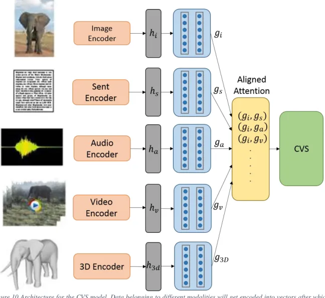
The common vector space architecture (CVS) takes in data belonging to different modalities and dimensions and maps them on to a lower-dimensional common embedding space. The CVS model is developed for two modalities and extended up to five modalities. The CVS uses different encoders to extract feature vectors and uses fully connected neural networks to map into the common space. Figure 8 shows the architecture overview of the CVS model with five input modalities. CNNs are used as the default encoding network for images and videos, audios are encoded using MFCC features whereas text data can be encoded using a bag of words model or a sentence-to-vector representation such as SkipThoughts [13].
These encoders convert a higher dimensional data from fully connected layers, into a vector representation to further reduce the dimensions of these vectors. To simplify, (3.1.1) shows the generic transformation of the input into the CVS representation. X is the input data which could either be images, text, video, audio or 3D, E is the common vector space representation, WE is the encoder weight matrix, and WT is the weight matrix that transforms the feature vector into the common embedding vector representation.
𝐸 = 𝑊
𝑇(𝑊
𝐸𝑋
)
(3.1.1)
Figure 10 depicts the architectural set up of the CVS model. In Figure 9, the vector representations are indicated by hi, ht, ha, hvand h3d. Each modality has its separate encoder
that converts the raw data into a vector representation. These vector representations are of different dimensions. For example, hi is a 4k vector from ResNet [6], while ha is a 29
dimensional MFCC feature, and so on. To bring all modalities to the same dimensions, we add two fully connected neural network layers, each containing 512 neurons. These layers along with the attention layer are initialized randomly and trained to minimize the total loss of the system.
26 | P a g e
Figure 10 Architecture for the CVS model. Data belonging to different modalities will get encoded into vectors after which they are projected into the common embedding space using fully connected layers.
Once the input data is projected onto the CVS, we use the cross-entropy loss function to perform classification and use metric learning losses simultaneously to cluster the samples. In this embedding space, the points are rearranged such that the total entropy of the system is minimized. In the CVS, objects that belong to the same category are mapped close to each other and well separated from objects that belong to some other category irrespective of their modality.
For example, the images, text, and videos of an elephant will be well separated from the images, audio, and video of a plane. The objective of the training is to minimize the inter-cluster distance and maximize the intra-inter-cluster distance. The distance between any two vectors can be calculated as the Euclidian distance as shown in (3.1.2) or the cosine distance between
27 | P a g e two vectors as shown in (3.1.3). Figure 11 gives us an intuitive idea of how cosine distance works. The cosine distance gives importance to the angular rotation between two vectors and gives a similarity score.
Figure 11 Cosine distance between two vectors in a 2D representation.
𝑑 = ||𝑓
𝑖− 𝑓
𝑗||
22(3.1.2)
𝑑 =
cos (𝑓𝑖 ,𝑓𝑗 )||𝑓𝑖 ||.||𝑓𝑗 ||
(3.1.3)
A.
Loss Functions
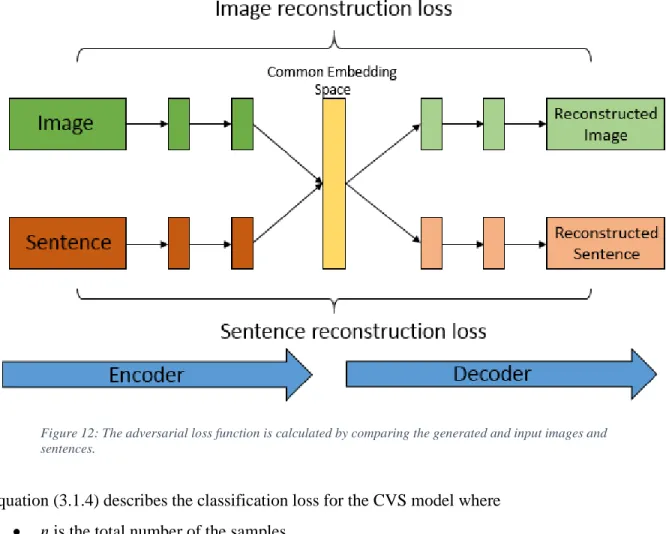
The CVS uses three loss functions to minimize the entropy of the common space. These loss functions are common across the variations of the model that we describe in Sections 3.2 and 3.3. Figure 12 shows the adversarial loss function in this context of this model. The adversarial loss function has two separate loss values that are back propagated. The image reconstruction loss tries to minimize the difference between the input image embedding and the output image embedding while the sentence reconstruction loss minimizes the difference in the sentence embeddings.
28 | P a g e
Figure 12: The adversarial loss function is calculated by comparing the generated and input images and sentences.
Equation (3.1.4) describes the classification loss for the CVS model where
n is the total number of the samples, y is the ground truth
f(s) is the sigmoid function as shown (3.1.5).
𝐿
𝑐= −
1 𝑛∑
(𝑦
𝑖𝑙𝑜𝑔 𝑓
𝑖(𝑠) + (1 − 𝑦
𝑖) (1 − 𝑙𝑜𝑔 𝑓
𝑖(𝑠))
𝑛 𝑖=1)
(3.1.4)
𝑓(𝑠) =
𝑒𝑠𝑖 ∑ 𝑒𝐶 𝑠𝑗 𝑗(3.1.5)
29 | P a g e
A modified version of the triplet loss described in Section 2.5 is used in (3.1.6). The triplet loss we implement has two parts: inter-modal and intra-modal triplet loss. The loss is calculated for two modalities at a time. The inter-modal loss consists of the triplets between the two modalities. The intra-modal loss will calculate the triplet loss for the data points belonging to the same modality. We use a weighted sum of these losses to calculate the total triplet loss.
𝐿𝑡 = ∑ 𝛾1 ∑ 𝑚𝑎𝑥(0, |𝑓𝑎𝑥− 𝑓 𝑝𝑥| 2 − |𝑓𝑎𝑥− 𝑓 𝑛𝑥|2 + 𝛼1) 𝑖,𝑠,𝑣,𝑎,3𝑑 𝑥,𝑦 + 𝛾2 ∑ 𝑚𝑎𝑥(0, |𝑓𝑎𝑦− 𝑓𝑝𝑦| 2 − |𝑓𝑎𝑦− 𝑓𝑛𝑦|2 + 𝛼2) + 𝛾3 ∑ 𝑚𝑎𝑥(0, |𝑓𝑎𝑥− 𝑓𝑝𝑦| 2 − |𝑓𝑎𝑥− 𝑓𝑛𝑦|2 + 𝛼3)
(3.1.6)
Where: |𝑓𝑎𝑥− 𝑓𝑝𝑥| 2is the distance between the anchor and positive sample.
|𝑓𝑎𝑥− 𝑓
𝑛𝑥|2is the distance between the anchor and negative sample. α1, α2, α3 are the margins for the triplet loss.
γ1, γ 2, γ 3: arethe individual weights of the 3 losses.
A weighted combination of Lc and Lt andare used in (3.1.8) to calculate the total toss of the
system where α and 𝛽 are individual weights given to these two loss terms. We observe that the adversarial loss does not improve the model much. In fact, when used individually, it is unable to perform at the required level. We further discuss this phenomenon in Chapter 5.
𝐿 = α
𝐿
𝑐+ 𝛽𝐿𝑡(3.1.7)
B.
Training Strategy
Similar to most deep learning networks, the CVS is trained in batches. In the implementation of the triplet loss, for any iteration, an anchor, positive and negative sample is selected. Since the CVS model can handle up to five modalities, this selection happens in batches continuously till we have traversed through the entire dataset. In the CVS setting, all the information for all
30 | P a g e
the modalities is given to the model at the initial stage. If new data is to be added to the network, the entire network has to be re-trained.
In the CVS setting, we will always need (𝑛2) attention blocks where n is the total number of modalities. In the case of n = 5, we need 10 attention blocks.
Such a training methodology means that the CVS architecture can only be built once we have all the data that is going to be used.
C.
Aligned Attention
Attention has proven to be an effective mechanism in aligning two vectors. The alignment provides a way to map local features across the two modalities. Attention has shown to be effective in tasks such as image captioning [39, 40]. For a given duplet of vectors, attention calculates a similarity score et(i) for every feature in the vector where i is the ith feature and t is
time step. Computation of et
i is shown in (3.1.7)
𝑒
𝑖𝑡 =𝑊
𝑇(𝑊
𝑎ℎ
𝑡−1+ 𝑈
𝑎𝑣
𝑖+ 𝑏
𝑎)(3.1.8)
Where
ht-1is the previous hidden state. Viis the ithfeature.
Wa, Wt, Ua, baare all learnable parameters.
eti is then passed through a softmax layer as (3.1.8). The final feature is a weighted combination
of all the N input features as shown in (3.1.9).
𝑎
𝑖𝑡=
exp (𝑒𝑖𝑡)∑𝑁𝑘=1 exp (𝑒𝑘𝑡)
(3.1.9)
𝜃𝑡(𝑉) =
∑
𝑁𝑎
𝑖𝑡31 | P a g e
𝜃𝑡(𝑉) is used as the final output of the attention layer which transforms the input vector into a new aligned vector that is better aligned with each other.
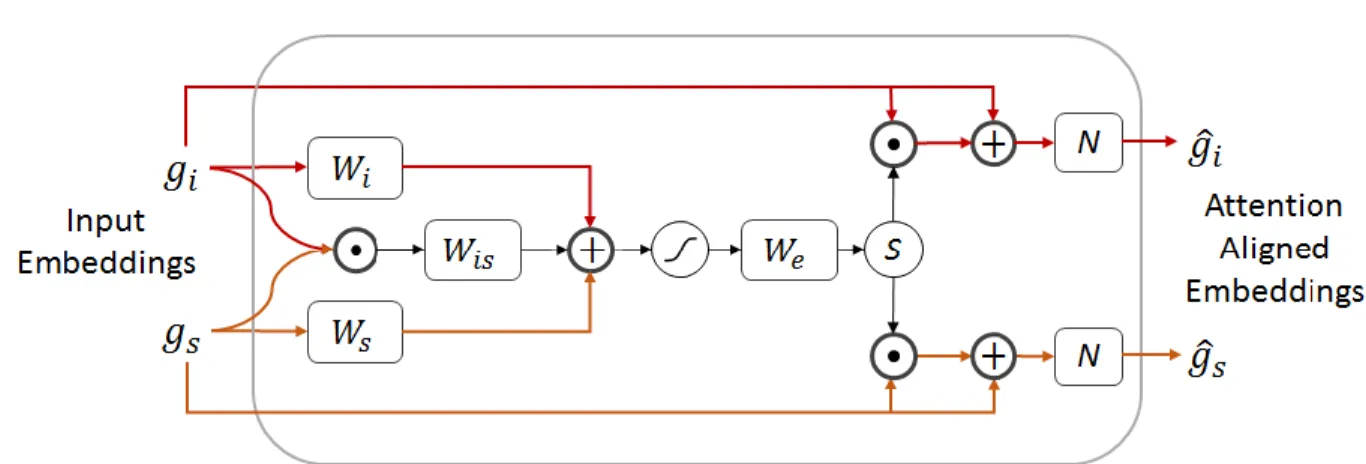
In the multi-modal CVS setting, the output of the encoder network is fed to the attention model. The attention model as shown in Figure 13 takes in two input embeddings and transforms into an attended embedding. These embeddings are L2 normalized at the output stage before being
projected into the CVS space. For any given two modalities, there has to exist one attention block between them. This pairwise attention block ensures that a pair of data points that belong to the same class are well aligned. Equation (3.1.10) shows how two input embeddings are converted to a single value at any given time step.
gi – input embedding of modality 1. gs– input embedding of modality 2.
gis– the element-wise product of giand gs. Wi, Ws, We– learned weights.
Equation (3.1.12) passes
𝑒
𝑖𝑠𝑡 through a softmax layer.𝑒
𝑖𝑠𝑡 is the same dimension as the CVS dimension.∑ exp (𝑒
𝑖𝑠𝑡)
is a scalar quantity that is the sum of all the elements in the𝑒
𝑖𝑠𝑡 vector. Thus, equation (3.1.12) provides the softmax functionality. In the attention mechanism, we insert a ResNet like skip connection so that the weight matrices just have to learn the difference between the input and the output and not the entire transformation itself. This reduces learning time and improves results in our experiments and is a key component of the aligned attention block.𝑒
𝑖𝑠𝑡 =𝑊
𝑒𝑡𝑎𝑛ℎ(𝑔
𝑖𝑊
𝑖+ 𝑔
𝑠𝑊
𝑠+ 𝑔
𝑖. 𝑔
𝑠𝑊
𝑖𝑠)(3.1.11)
𝛼
𝑖𝑠𝑡=
exp (𝑒𝑖𝑠𝑡)∑ exp (𝑒𝑖𝑠𝑡)
(3.1.12)
Equation (3.1.13) and (3.1.14) shows the output of the attention block. The
𝛼
𝑖𝑠𝑡 is multiplied with the input and added to the output.𝑔
𝑖= 𝑔
𝑖+ 𝛼
𝑖𝑠𝑡. 𝑔
32 | P a g e
𝑔
𝑠= 𝑔
𝑠+ 𝛼
𝑖𝑠𝑡. 𝑔
𝑠(3.1.14)
Figure 13 Aligned attention block which takes in two inputs and gives two corresponding outputs.
D.
Limitations of the CVS Model
The CVS model has some limitations:
Every time a new modality is added to the CVS, the entire architecture will be reset and we need to restart training from scratch.
There is no provision in the structure of the CVS to perform incremental stage-wise training.
Since the model will re-train, we lose traction of the existing inferences. This makes the CVS model inflexible to the addition of new modalities.
We try to address some of these issues by introducing Multi-staged Common Vector Space (M-CVS) and Reference Vector Space (RVS) respectively, in Sections 3.2 and 3.3.
3.2
Multi-Staged Common Vector Space (M-CVS)
The Multi-Staged Common Vector Space (M-CVS) is a space that is the same as the CVS except the training procedure is different. The objective here is still the same as the CVS and similar objects and concepts will lie close to each other in this M-CVS. To overcome the shortcomings of the CVS model, we develop a training strategy that builds the CVS architecture in a stage-wise manner. The M-CVS model network is able to add newer modalities of data in a stage-wise manner without having to retrain or change the existing network architecture. This means that the M-CVS model can be initially trained on two
33 | P a g e
modalities and at a later time, an additional third, fourth and fifth modality can be added without having to change the original two modality network.
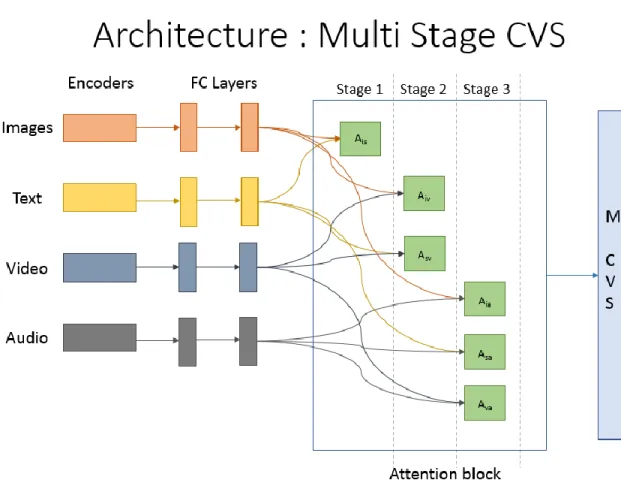
In the M-CVS model, the updating of weights in the back-propagation is controlled such that only weight matrices belonging to the new modality of data are updated whereas the other weights remain unchanged. For such an architectural setup, n new attention blocks are added in every stage.
Figure 14 shows the architecture of the multi-stage CVS model. The data belonging to different modalities passes through separate encoding networks and fully connected layers before being passed into the M-CVS layer. In every subsequent stage, newer modalities along with the new attention blocks are added. For example, in stage 2, the video modality is added to the M-CVS model and an additional two attention blocks are introduced. The attention block used in the M-CVS model is the same as described in Chapter 3.
A.
Training Strategy
The M-CVS model uses the same feature extractors as the CVS model. The advantage of defining the M-CVS is that it allows the addition of new information to the vector space without disturbing existing information in the space. For instance, if the image and text modalities were present in the M-CVS, the addition of the video modality will not affect the existing transformation between the images and text modalities.
34 | P a g e
Figure 14 Architecture for the Multi-Stage CVS Model. Every additional stage takes n new attention blocks.
3.3
Reference Vector Space (RVS)
The Reference Vector Space (RVS) is again, conceptually the same as the CVS and the M-CVS. The RVS goes one step further in restricting the number of attention blocks required at each stage. The main idea of the RVS is to be able to have one transformation for every modality into the common embedding space. The RVS is inspired by the International Color Consortium’s device independent profile connection space where inputs from multiple sources are mapped to a common reference color specification that allows easy transfer from one color space to any other.
In the RVS, we define one reference modality to which all other modalities will be mapped to. This allows the mapping of all new modalities through this singular reference modality. Similar to the CVS and the M-CVS architecture, the goal is to have similar objects and concepts lie close to each other in clusters that are well separated from groups of other concepts and objects in the RVS. Figure 15 shows the architecture set up of the RVS model where only one additional attention block is required to map the new modality into the RVS.
35 | P a g e
A.
Aligned Attention for RVS
The attention mechanism developed for the RVS model is such that there are only n
attention blocks for n modalities. In the CVS model, there were (𝑛2) attention blocks whereas, in the M-CVS model, there are n additional blocks for a newly added modality. For the RVS model, there is only 1 additional attention block added per new modality. Figure 16 describes the modified attention mechanism for the RVS. Equation 3.3.1 describes the calculations for the aligned attention for the RVS.
36 | P a g e
Figure 16 Attention mechanism for the RVS model.
We use a similar attention model as described in Chapter 3 but modify it to satisfy the needs of the RVS. We break down the We from 3.1.11 into two parts Wieand Wse where Wie is the reference weight that does not change after the initial training. However, Wse
changes after the addition of every modality. So, for each additional modality that is added to the architecture, we will add a new Wse .
𝑒
𝑖𝑒𝑡 =𝑊
𝑖𝑒𝑡𝑎𝑛ℎ(𝑔
𝑖𝑊
𝑖+ 𝑔
𝑠𝑊
𝑠+ 𝑔
𝑖. 𝑔
𝑠𝑊
𝑖𝑠)(3.3.1)
𝑒
𝑠𝑒𝑡 =𝑊
𝑠𝑒𝑡𝑎𝑛ℎ(𝑔
𝑖𝑊
𝑖+ 𝑔
𝑠𝑊
𝑠+ 𝑔
𝑖. 𝑔
𝑠𝑊
𝑖𝑠)(3.3.2)
𝛼
𝑖𝑒𝑡=
exp (𝑒𝑖𝑒𝑡) ∑ exp (𝑒𝑖𝑒𝑡)(3.3.3)
𝛼
𝑠𝑒𝑡=
exp (𝑒𝑠𝑒𝑡) ∑ exp (𝑒𝑠𝑒𝑡)(3.3.4)
Equations (3.3.5) and (3.3.6) show the output of the attention block. The
𝛼
𝑖𝑠𝑡 is multiplied with the input and added to the output.37 | P a g e
𝑔
𝑠= 𝑔
𝑠+ 𝛼
𝑠𝑒𝑡. 𝑔
𝑠
(3.3.6)
3.4
Stage Wise Learning for Multi Modal Embeddings
To overcome the limitations of the lesser number of multi-modal datasets, we develop a model that performs the stage-wise addition of information into the vector space. The subsequent addition of new information can be considered as the new modalities that are being added to the space. In the stage-wise learning method, we train our model on subsets of the dataset and then incrementally keep adding additional information into the model. The stage-wise learning technique can be thought of as a way of pre-training the network. For example, in the first stage, we add information about only 10 classes and train the model. In the subsequent stage, we use the model from the previous stage and add new class information to the network by training it for these additional new classes. We evaluate this model on two sets of data: 1. A subset of the test data which included only the information from the first stage of training. 2. The entire holdout test dataset.
In ‘1.’, we expect the recall scores to decrease across the stages whereas the model becomes more generalized. In the first stage, it would have overfitted on the initial classes it was trained on but as the stages progress, the overfitting problem will be resolved. In ‘2.’, the model will initially perform poorly on the entire test set because it has seen very few classes and the model is not robust. However, as the training stages progress, we can see it improving because as the model sees more classes, it starts performing better on the test dataset. We limit our work and experiments in this architecture to the image and text modalities only.
38 | P a g e
Figure 17: Step by step implementation of stage-wise learning.
A.
Training Strategy
The training strategy is described in Figure 17. Consider a training set containing N categories. We divide these categories into groups of K categories each. In the first stage, K categories are trained. In the subsequent stages, further K categories are added to the network. At each stage, the loss is calculated with respect to the K categories that are being added.
Stage 1:
Train on first
k modalities
Stage 2:
Add a new
set of k
modalities
Stage 3:
Add a new
set of k
modalities
…
Final Stage:
Add the last
set of
classes to
the
architecture
39 | P a g e
Chapter 4
Implementation
4.1
Datasets
We use multiple multi-modal datasets to test our architecture. Commonly, most datasets consist of two modalities. We evaluate the CVS, M-CVS and RVS space on two multimodal datasets and the CVS on the two cross modal datasets.
A.
XMedia [11, 47] and XMediaNet [51,59]
The XMedia dataset contains five different modalities of data. It contains images, text, audio, video and 3D point data. The number of samples in each of the modalities is stated in Table 1. XMedianet is an extension of the XMedia dataset which has the same modalities of data but with more data points. The numbers in Table 1 indicate the training and testing split for both the datasets. The XMedia and XMediaNet dataset come as pre-extracted features as shown in Table 2. The 200 categories in the XMediaNet dataset are classified into primarily two parts: animals and artifacts. While animals like elephant, owl, honey bees make up 48 out of the 200 categories, the artifacts make up the remaining 152 categories including things like violin, airplane, shotgun, camera, etc. Figure 18 and Figure 19 display samples from the XMedia and XMediaNet datasets respectively.
40 | P a g e
41 | P a g e
Table 1: XMedia and XMediaNet dataset statistics. Figures indicate the number of training and testing samples.
XMedia XMediaNet Image 4000, 1000 32000, 8000 Text 4000, 1000 32000, 8000 Video 400, 100 8000, 2000 Audio 800, 200 8000, 2000 3D 400, 100 1600, 400 Categories 20 200
42 | P a g e
Table 2: XMedia and XMediaNet Features and their dimensions.
XMedia XMediaNet Dimensions
Image CNN CNN 4096
Text Bag of Words Bag of Words 2048
Video CNN CNN 4096
Audio MFCC MFCC 29
3D LightField LightField 4700
B.
Nuswide [49] and Pascal [50]
The Nuswide and Pascal datasets contain images and their corresponding text data. Each of the images and text samples belongs to one category and we perform retrieval for an input query image or text. Figure 20 displays samples from the Nuswide dataset and Table 3 describes the dataset statistics for the Nuswide and Pascal datasets.
Figure 20: Sample images from the Nuswide dataset. [49]
C.
Birds [58]
We show zero-shot retrieval on the Birds dataset to evaluate the performance of the stage-wise learning model. The Birds dataset contains 150 categories for training and 50 unseen categories for testing. The goal of the zero-shot retrieval is to understand if the model is able to perform well on unseen categories and if the clusters that are being formed are robust or not. For the stage-wise learning methods, we split the Pascal and Nuswide datasets into groups of five classes and implement stage-wise learning on these groups. Additionally, we also report
43 | P a g e
stagewise learning scores for the zero-shot learning on the Birds dataset. Table 4 describes the dataset statistics for the Birds.
Table 3: Pascal and Nuswide dataset statistics. Figures indicate the train and test splits.
Pascal Nuswide
Image 800, 200 8000, 2000
Text 800, 200 8000, 2000
Categories 10 20
D.
Table 4: Train and test split for the Birds dataset used to perform zero-shot retrieval.
Birds
Train 8855, 2933
Categories 150, 50
4.2
Implementation
We implement cross-modal retrieval on these datasets using gradient descent based techniques where the goal is to minimize the loss functions described in Section 3. We pre-extract the vector representations of all our data. We use ResNet architecture to extract the image features and SkipThoughts to extract the text features for the cross modal retrieval task. For the multimodal retrieval task, we use the features enlisted in Table 2. We use Tensorflow on Nvidia GPUs to perform all our experiments and use a 512 dimension common embedding space. Our batch size is fixed at 128 with a learning rate of 0.001. For the triplet loss, we set all the margins (α1, α2, α3) to 1.0. We set γ1, γ2, γ3 to 0.25 and 0.25, 0.5 respectively.
A.
Evaluation Metric
Precision, recall, F1 score, accuracy are some of the most popular model evaluation metrics. In a task like retrieval, we want to measure the precision of our model for every query. In case of multiple queries, we want to define a metric that that represents the performance of the model for all the queries. That is why, mean average precision is the chosen metric in the area of information retrieval.
44 | P a g e
We calculate the average precision value for the top K queries.
𝐴𝑃 =1N∑𝐾𝑛=1(𝑝(𝑟). 𝑟𝑒𝑙(𝑟))
(4.2.1)
Where:
N is the number of relevant data samples in the retrieved results.
p(r) is the precision at r and rel(r) is a flag that indicates if the retrieved result is a match or not.
The mAP is obtained by averaging the AP of all the queries. We report the mAP at 50 (K = 50)
on all our experiments.
B.
Intuitive Understanding of mAP
Retrieval is primarily the task of searching for information that is very similar to the query. Figure 21 depicts an intuitive way of understanding how this metric is calculated. Mean average precision is a standard metric used to measure the performance of a retrieval system. Let Q be a user query, G be a set of labeled data in our common embedding space and d(i,j) be a measure of the similarity between two objects i,j. Let G’ be the ordered set of G according to the function d(i,j) and k be an index of G’.
45 | P a g e
In the above query, the average precision for the Q is given by:
𝐴𝑃 =(1.0 + 0.5 + 0.6) 3
Similarly, the AP is calculated for the queries in the test set and mAP is the average of all the APs.
46 | P a g e
Chapter 5
Results and Analysis
5.1
Results
In this section, we compare all the implementations discussed in Chapter 3 on the datasets discussed in Chapter 4. We report mAP@50 scores and different visualizations to analyze our results.
A.
CVS Model: Pascal and Nuswide
We evaluate our CVS model on the Pascal and the Nuswide datasets. We observe that the addition of the aligned attention mechanism improves retrieval as is evident from the scores. The aligned attention gives an improvement of 15% over the baseline CVS model.
Table 5: mAP scores for the Pascal and Nuswide dataset.
Dataset Method img2txt txt2img
Pascal UNSCM 0.304 0.282 Deep-SM 0.446 0.478 ACMR 0.535 0.543 DCKT 0.582 0.587 MCSM 0.598 0.597 CBT 0.602 0.583 DSCMR 0.710 0.722 Baseline CVS 0.591 0.567 CVS + Aligned Attention 0.660 0.671 Nuswide UNSCM 0.312 0.354 CCL 0.506 0.535 CSGH 0.542 0.569 ACMR 0.544 0.538 SC ACMR 0.545 0.448 DCKT 0.556 0.584 UGACH 0.631 0.641 DSCMR 0.611 0.615 Baseline CVS 0.450 0.485 CVS + Aligned Attention 0.574 0.676
47 | P a g e
B.
CVS Model: XMedia and XMediaNet (2 modalities)
Table 6 displays the scores on the XMedia and XMediaNet when it is trained only on image and text modalities.
Table 6: mAP scores for the Xmedia and XMediaNet dataset.
Dataset Method img2txt txt2img
Xmedia CBT 0.516 0.464 CM-GAN 0.567 0.551 Baseline CVS 0.895 0.902 CVS + Aligned Attention 0.908 0.950 XmediaNet CBT 0.516 0.464 CM-GAN 0.567 0.551 Baseline CVS 0.536 0.495 CVS + Aligned Attention 0.598 0.583
C.
CVS Model: Xmedia and XMediaNet (5 modalities)
Table 7 represents the scores on the XMediaNet when it is trained on all the modalities. The scores for images and sentences are much higher because of the higher number of training samples in each of these modalities. The larger corpus of training data for these two modalities means that the model is able to generalize well across a large spectrum of data. The same cannot be said about videos as it has fewer samples to train on (see Table 2).
Table 7: mAP scores for the images, text, and video for the XMediaNet dataset.
Attention I S V No I 0.688 0.417 S 0.616 0.347 V 0.306 0.281 Average 0.442 Yes I 0.775 0.605 S 0.685 0.504 V 0.395 0.383 Average 0.558
Table 8 shows the scores on the XMedia when it is trained on all the modalities. Similar to the XMediaNet dataset, the scores of images to sentence and sentence to image retrieval are high owing to the vast amount of training data that is present in these two modalities.
48 | P a g e
Table 8: Cross modal retrieval scores (mAP) for the five modalities in the XMedia dataset.
Method Q - R I T A V 3D CVS I - 0.895 0.759 0.606 0.624 T 0.902 - 0.763 0.550 0.637 A 0.504 0.480 - 0.293 0.446 V 0.138 0.317 0.253 - 0.153 3D 0.436 0.580 0.412 0.129 - Avg 0.494 CVS + Attention I - 0.908 0.708 0.801 0.731 T 0.95 - 0.743 0.828 0.769 A 0.416 0.477 - 0.341 0.42 V 0.49 0.481 0.366 - 0.434 3D 0.58 0.545 0.457 0.558 - Avg 0.600
To coalesce the twenty different retrieval scores, we evaluate a model based on the average performance across all these modalities. We observe that the CVS model with the aligned attention works best and gives an average retrieval score of 0.6. The 3D and audio modalities have fewer samples and low dimensionality respectively and hence the scores for these two modalities are comparatively lower. Figure 22 describes the decrease in the total loss as training progresses.
49 | P a g e
D.
M-CVS Model: Xmedia and XMediaNet (5 modalities)
In the M-CVS model, we implement a four-stage learning approach for the XMedia dataset. The four stages help build the model such that each new stage does not affect previous stages of training. The four stages of training are described below.
Stage 1: Train images and text modalities.
Stage 2: Perform incremental addition of the video modality. Stage 3: Add audio modality to the architecture.
Stage 4: Add 3D modality to the stage-wise learning architecture.
The scores reported in Table 9 are the scores after the fourth stage of training. These scores are comparable with the CVS model.
Table 9: Cross modal retrieval scores(mAP) for the M-CVS model on the XMedia datadset.
Method Q - R I T A V 3D S2UPG I - 0.27 0.265 0.264 0.394 T 0.275 - 0.242 0.242 0.338 A 0.274 0.244 - 0.207 0.363 V 0.225 0.193 0.168 - 0.267 3D 0.345 0.275 0.329 0.276 - Avg 0.273 SCVM I - 0.903 0.406 0.532 0.655 T 0.889 - 0.507 0.549 0.722 A 0.438 0.527 - 0.313 0.37 V 0.553 0.58 0.302 - 0.45 3D 0.603 0.679 0.37 0.426 - Avg 0.539 M-CVS I - 0.897 0.531 0.809 0.782 T 0.943 - 0.538 0.840 0.822 A 0.508 0.513 - 0.202 0.505 V 0.521 0.211 0.318 - 0.282 3D 0.616 0.627 0.338 0.537 - Avg 0.567
In the XMediaNet dataset, we perform just a 2 stage of training for the training. In stage 1, we train image and text modalities and then add the video modality. While this model doesn’t perform as well as the CVS model, it still performs better than the CVS model without the aligned attention
50 | P a g e mechanism. Figure 23 shows the decrease in the metric loss across subsequent epochs for the M-CVS model.
Table 10: mAP scores for images, text, and video for XMediaNet dataset.