UC San Diego
UC San Diego Electronic Theses and Dissertations
TitleModeling User Behavior Patterns in LBSNs: A Graph Embedding Approach Permalink https://escholarship.org/uc/item/8hw3d1t3 Author Xu, Weiqi Publication Date 2019 Peer reviewed|Thesis/dissertation
UNIVERSITY OF CALIFORNIA SAN DIEGO
Modeling User Behavior Patterns in LBSNs: A Graph Embedding Approach
A Thesis submitted in partial satisfaction of the requirements for the degree Master of Science
in
Electrical and Computer Engineering (with a specialization in Intelligent Systems, Robotics, and Control)
by Weiqi Xu
Committee in charge:
Professor Julian McAuley, Chair
Professor Truong Quang Nguyen, Co-Chair Professor Nikolay Atanasov
Copyright Weiqi Xu, 2019 All rights reserved.
The Thesis of Weiqi Xu as it is listed on UC San Diego Academic is approved, and it is acceptable in quality and form for publication on microfilm and electronically:
Co-Chair
Chair
University of California San Diego
DEDICATION
TABLE OF CONTENTS
Signature Page . . . iii
Dedication . . . iv
Table of Contents . . . v
List of Figures . . . vii
List of Tables . . . viii
Acknowledgements . . . ix
Abstract of the Thesis . . . x
Chapter 1 Introduction . . . 1
1.1 Motivation and Challenges . . . 1
1.2 Our Work and Contributions . . . 4
1.3 Thesis Organization . . . 6
Chapter 2 Background . . . 7
2.1 Characteristics of Location-based Social Networks . . . 7
2.2 Influential Factors . . . 9
2.3 Distributed Representation Learning and Graph Embedding Methods 12 2.3.1 Factorization-based Approaches . . . 12
2.3.2 Random Walk-based Approaches . . . 14
2.3.3 Deep Neural Networks-based Approaches . . . 17
2.3.4 LINE-based Approaches . . . 18
2.4 Cold Start Problem . . . 19
Chapter 3 Data Exploration . . . 21
3.1 Dataset Statistics . . . 21
3.1.1 Foursquare . . . 21
3.1.2 Google Local . . . 22
3.2 Data Characteristics and Properties . . . 23
Chapter 4 Methodology . . . 31
4.1 Predictive Tasks . . . 31
4.2 Graph-based Embedding Model . . . 33
4.2.1 Bipartite Graph Construction . . . 33
4.2.2 Heterogeneous Graph Embedding . . . 35
4.2.3 Homogeneous Graph Embedding . . . 38
4.3 Context-aware Prediction Framework with Dynamic Tracking of User
Preference . . . 41
Chapter 5 Experiments and Results . . . 44
5.1 Datasets . . . 44
5.2 Comparison Models . . . 44
5.3 Evaluation Methodology . . . 47
5.4 Sensitivity of Model Parameters . . . 49
5.4.1 Embedding Dimension & Number of Samples . . . 49
5.4.2 Granularity of Sequential Pattern . . . 50
5.5 Performance of Context-aware Next-POI Prediction . . . 51
5.5.1 Impact of Influential Factors . . . 51
5.5.2 Comparative Results . . . 55
5.5.3 Performance Analysis on Dynamic Preference Tracking . . 58
5.6 Performance of Cold-Start Recommendation . . . 59
5.7 Performance of Social Link Prediction and Friend Recommendation 61 5.8 Visualization of Embeddings . . . 62 Chapter 6 Conclusion . . . 64 6.1 Discussion . . . 64 6.2 Summary . . . 66 6.3 Future Work . . . 67 6.4 Acknowledgement . . . 67
Appendix A JGEL Source Code . . . 69
LIST OF FIGURES
Figure 2.1: Example of a Typical LBSN . . . 8
Figure 3.1: Geographical Distribution of Foursquare Venues . . . 24
Figure 3.2: Geographical Distribution of Google Local Venues . . . 24
Figure 3.3: Users’ Temporal Preference for Various Activities . . . 26
Figure 3.4: User Preference vs. Day-of-week on Foursquare . . . 26
Figure 3.5: User Preference vs. Day-of-week on Google Local . . . 26
Figure 3.6: Sequential Patterns of User Behaviors in Foursquare . . . 27
Figure 3.7: Sequential Patterns of User Behaviors in Google Local . . . 27
Figure 3.8: Average Jaccard Similarity Between Friends and All Users . . . 29
Figure 4.1: Bipartite Graphs Constructed From Sample Records . . . 36
Figure 5.1: Sensitivity Analysis of Model Parameters . . . 50
Figure 5.2: Analysis on the Impact of Individual Factors . . . 53
Figure 5.3: Prediction Accuracy of Comparison Models . . . 56
Figure 5.4: Learning curves of NBC v.s. JGEL on Foursquare . . . 57
Figure 5.5: Performance on Cold-Start POIs . . . 60
Figure 5.6: Performance of Social Link Prediction . . . 60
Figure 5.7: Visualization of POI Embeddings of Different Time Slots . . . 63
LIST OF TABLES
Table 3.1: Foursquare Data Description and Examples . . . 22
Table 3.2: Google Local Data Description and Examples . . . 22
Table 3.3: Data Statistics Before and After Filtering . . . 23
Table 3.4: Data Statistics of Cold-Start POIs . . . 30
Table 4.1: Sample Check-in Records . . . 36
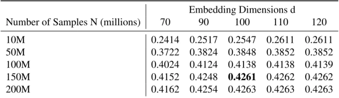
Table 5.1: Embedding Dimension VS. Number of Samples . . . 49
Table 5.2: Prediction Accuracy with Different Time Intervals . . . 50
Table 5.3: Impact of Individual Graph on Next-POI Prediction in Foursquare . . . 52
Table 5.4: Impact of Individual Graph on Next-POI Prediction in Google Local . . . . 54
Table 5.5: Prediction Accuracy of Comparison Models . . . 55
Table 5.6: Prediction Performance on Cold-Start POIs . . . 59
ACKNOWLEDGEMENTS
I would like to acknowledge Professor Julian McAuley for his support as the chair of my committee. His guidance has helped me shape my work into what it is.
I would also like to acknowledge Professor Truong Quang Nguyen as the co-chair, and Professor Nikolay Atanasov as my committee. I am gratefully indebted to their valuable comments on this thesis.
Finally, I must express my very profound gratitude to my parents and to my boyfriend for providing me with unfailing support and continuous encouragement throughout my years of study and through the process of researching and writing this thesis. This accomplishment would not have been possible without them.
ABSTRACT OF THE THESIS
Modeling User Behavior Patterns in LBSNs: A Graph Embedding Approach
by
Weiqi Xu
Master of Science in Electrical and Computer Engineering (with a specialization in Intelligent Systems, Robotics, and Control)
University of California San Diego, 2019 Professor Julian McAuley, Chair Professor Truong Quang Nguyen, Co-Chair
With the emerging of various location-based social networks (LBSNs), the study on user mobility patterns and many related tasks have become heated research topics, such as personalized location recommendation and friend recommendation. Many factors affect users’ behavior patterns, such as geographical influence, temporal effect and semantic effect. However, most of the previous work on modeling user trajectories lacks consideration on treating these factors from a graph perspective, therefore fails to capture the potential correlations among the rich context. In this thesis, we demonstrate that using a heterogeneous graph-based model to jointly embed user
and POI attribute networks with a unified framework can well preserve the network properties. Multiple factors are embedded into a shared low-dimensional latent space where their joint effect and potential correlations can be well captured. We conduct extensive experiments on large real-world datasets to evaluate our model performance on several major tasks in LBSNs. The experimental results highlight the versatility of our method which shows higher recommendation effectiveness compared with the state-of-the-art baselines. In addition, a online updating strategy is proposed to incorporate new visiting records and dynamically track users’ latest preference in linear time. We also show that this framework has the inherent ability to handle cold-start recommendations, which is a non-trivial task considering the network sparsity of LBSNs. The scalability and flexibility of our framework indicate that this method is promising to be put into practical use.
Chapter 1
Introduction
1.1
Motivation and Challenges
With the prevalence of mobile devices and the emerging of various location-based social networks (LBSNs) such as Yelp and Foursquare, massive user visiting records are collected based on users’ voluntary reports. More and more users are getting used to check-in at point-of-interests (POIs), such as scenic spots, restaurants and museums, and share their experience. On the other hand, users rely on these networks to help them discover new places and activities, as well as new friends who share similar interests with them. In fact, the study on LBSNs has become a heated research area in recent years, which brings large profits not only to personal recommendation, but also to many high-level tasks, such as event prediction and regional traffic forecast.
The vast amount of check-in records makes it possible to study user mobility, and make personalized recommendations base on the learnt user preference and mobility pattern. However, the problem nature and the characteristics of LBSNs have posed many challenges:
∙ Context awareness: Different from traditional recommender systems such as e-commerce websites, the recommendations in LBSNs usually need to take spatiotemporal context into consideration when making predictions aside from users’ personal preference. In
another word, users tend to make different choices in different time and places. In addition, users’ mobility pattern exhibits sequential effect. For example, a user would first check-in at a shopping mall, then go to a restaurant, and watch a movie at the cinema later on a typical weekend; travelers might first check-in at the airport after landed, then check-in at a hotel straight after. Taking all these context information into consideration when making predictions is necessary.
∙ Dynamic Tracking: User preference changes over time. On the other hand, the sequential effect of POI transitions has a large impact on user mobility. Therefore, in order to provide satisfying predictions, the recommender system needs to respond to stimulus in real-time according to users’ latest preference and spatiotemporal context. Besides, training the entire model takes time and can be costly. Thus, an ideal model should have the ability of online training, which can dynamically incorporate new records, and track users’ latest preference without retraining the whole model.
∙ Mutual effects of social and POI networks: User relationships form the social network, and the POI attributes in LBSNs form the heterogeneous POI network. Both social network and POI network affect users’ visiting behaviors, and the two networks show mutual effects towards each other. Friends tend to share similar preference and have co-visitation behaviors. Thus, incorporating social relationships can facilitate POI prediction. On the other hand, people who share similar mobility patterns are more likely to become friends, which uncovers the possibility of making social link recommendations based on POI network. Therefore, building a joint framework which captures the mutual effects between the two networks is expected to facilitate related prediction tasks while can be challenging.
∙ Data Sparsity: Visiting a place is more costly than rating movies and items online, and the check-in records in LBSNs is collected based on users’ voluntary report. As a result, the data in LBSNs is much sparser than that of traditional recommender systems.
∙ Cold Start: In LBSNs, new places and activities emerges everyday. An ideal model should have the ability of incorporating newly emerged POIs and help users explore new places. In fact, cold-start recommendation is a non-trivial task in LBSNs which needs careful inspection.
Many work has been devoted to studying user mobility patterns in LBSNs while lim-itations exist. First of all, previous work incorporates a variety of influential factors to learn users’ behavioral patterns mostly by combining all the partial factors. For example, probabilistic graphical models [1] generate different distributions for the considerable influential factors; collab-orative filtering model simultaneously factorizes coupled tensors and matrices constructed from heterogeneous data sources [2] to perform multi-dimensional collaborative recommendations based-on user, activity, time and location. However, the objective functions of these models are not designed for the network structure of LBSNs, and the diverse nature of multiple factors makes it difficult to incorporate them with an integrated model. In fact, most of the work ends up building a complicated hybrid model, which fails to generalize to various scenarios. Second, among the many factors that affect user behaviors, sequential effect and geographical effect are mostly studied, while social influence is frequently ignored. Last but not least, traditional methods directly capture the interactions between user POI pairs, which fails to observe the global structure of the entire information network [3]. For example, Factorization Machine only optimizes the first-order proximity between user and POI by observing their direct interactions.
Methods which learn graph representations by embedding nodes into a lower-dimensional latent vector space have been attracting increasing attention in the recent years [4]. The perfor-mance has been proved to be promising in many tasks, such as text mining [5] and event detection [6].
1.2
Our Work and Contributions
In this work, we extend the state-of-the-art graph embedding method for next-POI predic-tion and social link predicpredic-tion in LBSNs. The proposed method models user social network and POI attribute network with a joint framework where their mutual effect are captured. Users, POIs and POI attributes are all treated as network nodes and embedded into a shared lower-dimensional latent space. The observed links between network nodes include user-user, user-POI, POI-category, POI-time, POI-region, POI-rating, and POI-POI, which capture users’ social connections, visiting history, categorical effect, temporal effect, geographical effect, semantic effect, and sequential effect in POI transitions respectively. By optimizing the first-order and second-order proximity between network nodes, the obtained embeddings not only preserve the local and global structure of the network, but can also leverage the sparsity problem in real-world datasets. In addition, the proposed framework is flexible to incorporate multiple factors and network attributes, and can scale to large real-world dataset. An online training strategy is introduced which can dynamically track users’ latest preference in linear time without harming the prediction accuracy.
We conduct extensive experiments on two large real-world datasets, and compare our model with representative algorithms based on Probabilistic theory, Factorization Machine and Deep Learning. Experimental results demonstrate our model’s superiority over other state-of-the-art comparison methods on several predictive tasks.
In context-aware next-POI recommendation, our method outperforms comparison models in terms of both prediction accuracy and efficiency. By incorporating the content information of the cold-start POIs, our model can directly learn the embeddings of cold-start POIs through the same framework without additional feature engineering or model modifications. In addition, experiments show that our model gives better performance in cold-start recommendations than strong baselines.
used to discover potential social links by measuring pairwise similarity. The intuition behind is that users’ shared preference on POIs is captured through observing the second-order proximity of user-POI links. In another word, users with shared neighboring POIs are embedded close to each other in the embedding space. In fact, people who have similar visiting history are more likely to share similar interest and become friends. Model evaluation proves that our prediction framework achieves better results than heuristic methods, and the user embeddings obtained from our model are more representative compared with those of baselines.
By embedding all the network nodes into a shared latent space, our method not only optimizes on the observed links, but is also able to capture potential correlations among them. This explains for the more promising results in cold-start recommendation and social link prediction where side information is limited.
For each predictive task, we further investigate the impact of different influential factors. Methods to better capture these effects in our embedding framework are also discussed.
To summarize, in this thesis, we:
1. extend the state-of-the-art graph embedding method to model user mobility patterns in LBSNs. A joint framework is introduced which captures the mutual effect between user social network and POI attribute network.
2. introduce an online learning strategy which can dynamically update user preference without retraining the entire model, and can provide context-aware recommendations according to users’ stimulus in real-time.
3. demonstrate the superiority of the proposed model in next-POI prediction, social link prediction, and gives promising results in cold-start recommendation.
4. investigate the impact of influential factors on the modeling of user mobility, and discuss the way to better capture these effects in our embedding framework.
1.3
Thesis Organization
The rest of work is organized as follows. In Chapter 2, we introduce the problem back-ground, and provide a detailed explanation on the motivation behind this work. In Chapter 3, we explore the statistics and characteristics of the datasets we study on, and investigate the most significant effects the datasets exhibit. In Chapter 4, we explain the predictive tasks we study in this work, then introduce the model formulation, including embedding methodology, training process and prediction strategy. In Chapter 5, we report the experimental results of our method along with other representative comparison models on all predictive tasks. Thorough discussions on the experimental results are also included. In Chapter 6, we conclude our work, discuss the limits and shed light on some future directions.
Chapter 2
Background
2.1
Characteristics of Location-based Social Networks
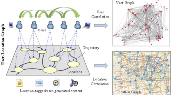
The emerging of location-based social network is a natural product of the development of location-based service. The location network contains massive amount of POIs along with their multiple attributes, including location, opening hours, and content information such as categories and user reviews. The social network is usually formed based on friendship, common interests, and shared knowledge. The LBSN is not a simple combination of the location network and social network where users can share POI-related information, it is partially observed and contains potential interactions between network nodes. The implicit connections are derived from users’ location-tagged check-in history, which includes timestamp, photos and reviews [7]. Figure. 2.1 [8] illustrates an example of a typical LBSN. As is illustrated in the diagram, the user network and location network are connected through visiting history to form the user-location graph, which contains location-tagged and user-generated content. The shared activities and mobility patterns among users indicate potential social closeness, while on the other hand, the mobility of similar users reveals content similarity among those locations.
Figure 2.1: Example of a Typical LBSN
users, locations and their interactions, and bring profits to many related tasks, such as community detection, event detection, preference- and context-aware location recommendation, and friend recommendation.
The most popular and well studied LBSNs datasets are Foursquare [9] and Gowalla [10] check-in data. Each check-in record contains user information, check-in time and POI side information. Users’ friend list is also included. Gowalla dataset a has larger size compared with Foursquare, but it lacks POI content information such as user reviews. These two datasets are collected based on users’ voluntary report, therefore suffer from severe data sparsity. Various types of tasks are studied, including location recommendation, social link prediction and user mobility tracking. Tarasov et al. [11] combine Foursquare check-in history with Twitter friend list to test their radiation model for location prediction task. In the work by Yao et al. [12], a recurrent model for next location prediction is proposed and evaluated on Foursquare check-in data collected from New York City and Los Angeles. Users with fewer than 50 records are removed, and only semantic trajectories within a 10h time interval are kept to obtain a denser network.
Aside from check-in data collected through users’ voluntary report, similar datasets that based on automatic collecting are also studied. For example, Huang et al. [13] worked on Wi-Fi access logs collected at Purdue University, which is much denser than Foursquare or Gowalla check-in data, and exhibits more significant temporal cyclic patterns.
2.2
Influential Factors
Among the many tasks in LBSNs, social link prediction and location recommendation have become popular research areas in the past few years. User mobility patterns is studied to learn personal preference, and rich POI attributes are frequently incorporated to provide valuable recommendation context. On the other hand, the side information helps to alleviate the sparsity problem of check-in data. For example, the insufficient observations of check-in activities can be compensated by tipping behaviors and rich text information such as reviews to infer user interests [14].
In social link prediction tasks, factors people usually consider to measure trajectory similarity [15] include location category [16], geographical distance [17], and co-occurrence with time and distance constraints, where the diversity of co-occurrence and popularity of locations were proved to show dominant effects and are most well studied. Pham et al. [18] introduce the notion of commitment and compatibility to measure similarity of users’ mobile patterns. The similarity quantifies social distances between users, which is used to infer real-world co-occurrences. In another work by Pham et al. [19], they further propose an entropy-based model which estimates the strength of social connections by analyzing people’s co-occurrences in space and time.
In location recommendation tasks, information used for context- and time- aware rec-ommendation includes social ties, geographical information, temporal information, and text description such as categories and reviews. Temporal and geographical information are most
well studied to learn users’ spatiotemporal preference or change in interest over time. Early work[20][21] argue that user preference is time-varying and has periodic patterns (e.g. day in a week). A direct approach is to add a dimension for time into the user-item adjacency matrix, then adopt Factorization-based methods [22], [2]. Yuan et al. linearly combine temporal cyclic patterns and geographical influence into a user-based collaborative filtering framework for time-aware POI recommendation. In another work done by Yuan et al. [23], preference propagation is applied on a geographical-temporal graph to realize time-aware location recommendation. Topic models are also widely adopted in time-aware recommendation. For example, [24] uses a topic model to learn users’ temporal preference by creating unique time features for every topic.
In the next-POI prediction problem, the sequential transitions between locations is an addition factor to consider, which shows significant effect. Markov chain is widely used to capture the sequential effect in user mobility. Zhang et al.[25] introduce a probability-based additive Markov-chain model based on the assumption that the latest activities have the greatest impact on user’s current preference. Another popular method is FPMC proposed by Rendle et al. [26]. It factorizes the tensor of transition cube consists of the transition probability matrices of all users. FPME [27] extends FPMC by modeling user-location distance and location-location distance in two different vector spaces. However, Markov chain methods are based on the assumption that the choice of next location is only affected by the previous location, which does not hold in the real-world scenarios. To track users’ entire check-in history, recurrent models are introduced, such as RNN, LSTM and GRU. Liu et al. propose a Spatial Temporal Recurrent Neural Networks (ST-RNN) [28], which can model continuous time intervals and geographical distance by constructing time-specific and distance-specific transition matrices in each layer of the neural network.
Recently, a lot of research has been devoted to inferring next-POIs through analyzing human mobility. Wang et al.v[29] indicate that the social proximity is strongly bound up with one’s mobility. The work in [30] distinguishes users’ different periodic mobility between work and home. [13] works on Wi-Fi access logs collected at Purdue University, and demonstrates
that students’ campus life exhibits more significant cyclic patterns. The work in [31] uses user mobility in LBSNs to measure the connectivity of various cities. More relevant work studying user mobility in LBSNs can be found in[32][33].
Some other work making use of other factors includes that of Liu et al. [34], which incorporates venue tags into a Matrix Factorization-based model for POI prediction.
The diverse nature of these influential factors poses challenges to incorporating them into a joint model. Many previous work comes up with hybrid models, where each individual component only captures one specific effect. In the work by Yang et. al [15], they first derive the network representation for each user with a probability-based generative model according to social links, then employ a RNN model and a GRU model to capture short-term and long-term effects of the sequential relatedness in users’ mobile trajectories respectively. The final model is a linear combination of all the partial representations of user and sequential context. Wang et al. [5] incorporates visual contents by first extracting image features using CNN, then add them into a probabilistic Matrix Factorization model to learn user and POI latent features. Hybrid models may show good prediction performance in the specific scenarios they’re designed for, while need careful feature engineering and lack the ability to generalize.
Joint frameworks do exist, such as aggregate LDA, Matrix Factorization-based and collab-orative filtering-based methods. Matrix or Tensor Factorization is a popular methodology that has been proved to be efficient and effective in POI recommendation tasks. Zhang et al. propose a multi-dimensional collaborative recommendation framework which uses Tensor Factorization techniques to capture temporal, categorical and geographical effects. Gao et al. [14] build a low-rank Matrix Factorization model which employs a sentiment-enhanced weighting framework when consider user sentiment indications, user-interest content and POI-property content. Zhao et al. [35] propose a unified LDA-based probabilistic model to learn user preference based on reviews, categories and geolocations of POIs. The model can also capture the interaction of sentiment, categorical and spatial information. Pasricha et al. [36] modify the traditional
Factor-ization Machine by replacing the inner product with the squared Euclidean distance to measure the interaction strength between features. The proposed model can operate on arbitrary feature vectors and is flexible to incorporate additional content information. Although these methods incorporate all the factors into a general framework, however, they neither cannot scale to large networks, nor their objective functions are not designed for capturing network structures, therefore not necessarily preserve the global network structure. [3]
In the next section, we will provide a detailed literature of some widely used graph embedding approaches for network embedding tasks. Their characteristics and limitations will be discussed. Finally, we will introduce the approach we use in this work, and provide some insights of the intuition behind our choice.
2.3
Distributed Representation Learning and Graph
Embed-ding Methods
In the recent years, graph embedding methods which represent networks along with their properties into a latent vector space have been attracting increasing attention. Specifically, these methods aim at learning graph representations of the networks by embedding nodes into a lower-dimensional vector space, where connected nodes are embedded close to each other in the embedding space [4]. In general, there are three main groups of approaches: Factorization-based, Random-Walk based and Deep Neural Network-based.
2.3.1
Factorization-based Approaches
The Factorization-based methods obtain the embeddings by factorizing the matrices representing the connections between network nodes. The most widely used matrices include adjacency matrix, transition probability matrix and Laplacian matrix. A representative work using
adjacency matrix is Locally Linear Embedding (LLE) [37], which is under the assumption that every node is a linear combination of its k-nearest neighbors in the embedding space. The weights of neighbors nodes forms the weight matrix𝑊, and the reconstruction error is defined as:
𝜀(𝑊) =∑ 𝑖 |𝑋⃗ 𝑖− ∑ 𝑗 𝑊𝑖𝑗𝑋⃗𝑗|2 (2.1) where: Σ𝑗𝑤𝑗 = 1
Mapping every point𝑋𝑖into a lower-dimensional representation𝑌𝑖, the objective turns into:
min 𝑌 Φ(𝑌) = ∑ 𝑖 |𝑌𝑖−∑ 𝑗 𝑊𝑖𝑗𝑌𝑗|2 (2.2)
whereΦ(𝑌)is further turned into:
Φ(𝑌) =∑
𝑖𝑗
𝑀𝑖𝑗(𝑌𝑖⋅𝑌𝑗) (2.3) where:
𝑀 = (𝐼−𝑊)𝑇(𝐼−𝑊)
After decentralization, the problem comes down to an eigenvalue decomposition problem, where the embeddings are the eigenvectors corresponding to the last 𝑚non-zeros eigenvalues of the positive semi-definite matrix𝑀.
The Laplacian matrix [38] is formed with Laplacian of the graph, which is more computa-tionally efficient, and can preserve local structure well. The basic idea is to make the representations of two similar nodes close to each other in the low-dimensional embedding space. The objective
function is:
min∑
𝑖𝑗
|𝑦𝑖−𝑦𝑗|2𝑊𝑖𝑗 = min𝑡𝑟𝑎𝑐𝑒(𝑌𝑇𝐿𝑌), 𝑠.𝑡.𝑌𝑇𝐷𝑌 =𝐼 (2.4) 𝐿=𝐷−𝑊 is the Laplacian matrix of the graph, where𝑊 is the adjacency matrix, and𝐷is the degree matrix (𝐷𝑖𝑗 =∑𝑛𝑗=1𝑊𝑖𝑗).
Some related models include Graph Factorization (GF) [39], High-Order Proximity Pre-served Embedding (HOPE) [40], and Structure Preserving Embedding (SPE) [41]. A further extension based on Factorization methods is Marginal Fisher Analysis proposed by Yan et al. [42]. Two types of graphs are introduced in this work: the intrinsic graph characterizes the intraclass compactness, while the penalty graph connects the marginal points between different classes and characterizes the interclass separability.
In general, Matrix Factorization methods obtain the embeddings by solving the leading eigenvectors of the affinity matrices, therefore suffer from high computational complexity and cannot scale to large real-world networks. Factorization Machine shows better scalability, while still, it only observe the direct interactions between network nodes, and fail to capture the global structure of the entire network. What’s more, Factorization-based methods are not capable of learning arbitrary functions [4]. Their objective functions are not designed for capturing network structures, therefore cannot learn structural equivalence or preserve global structure.
2.3.2
Random Walk-based Approaches
By comparison, Random Walk-based methods show the ability to capture higher order proximities among nodes and can handle partially observed large-scale networks.
The random walk task is essentially a discrete Dirichlet problem applied on the graph. A random walk path usually starts from a selected node in the network, then moves to the random neighbors from the current node for a pre-defined number of steps. The relative probability
distributions of the child nodes are computed by sampling a set of random walk paths from the graph. To be specific, given a graph𝐺(𝑉 , 𝐸), if a random walk starts from node𝑣0and reaches node𝑣𝑡after𝑡steps, the probability distribution can be represented as:
𝑃𝑡(𝑖) =𝑃 𝑟(𝑣𝑡=𝑖) (2.5) The transition probability matrix is𝑀= (𝑝𝑖𝑗)𝑖,𝑗∈𝑉, where
𝑝𝑖𝑗 = ⎧ ⎪ ⎨ ⎪ ⎩ 1∕𝑑(𝑖), if𝑖𝑗∈𝐸, 0, otherwise (2.6)
Therefore, the walking rule from one node𝑃𝑡to another node𝑃𝑡+1can be described as:
𝑃𝑡+1=𝑀𝑇𝑃𝑡 (2.7) DeepWalk was first proposed for language modeling based on word2vec and random walk, but it has also shown good performance in other networks such as social networks. DeepWalk preserves higher-order proximities between nodes by maximizing the probability of observing the neighbors of a node within a certain window conditioned on its embedding using stochastic gradient descent[6]. Under this scheme, nodes with similar neighbors are closely embedded in the embedding space.
The objective function can be described as:
(𝑠) = 1 𝑠 |𝑠| ∑ 𝑖=1 ∑ 𝑖−𝑡⩽𝑗⩽𝑖+𝑡,𝑗≠𝑖 log𝑃 𝑟(𝑣𝑗|𝑣𝑖) (2.8) where 𝑃 𝑟(𝑣𝑗|𝑣𝑖) = 𝑒𝑥𝑝(𝑣⃗𝑗 𝑇 ⋅𝑣⃗𝑖) ∑ 𝑣𝑘∈𝑉 𝑒𝑥𝑝(𝑣⃗𝑘 𝑇 ⋅𝑣⃗𝑖) (2.9)
where𝑣𝑗 is the neighboring nodes of node 𝑣𝑖 within a𝑡−𝑠𝑡𝑒𝑝𝑠 window, equation 2.9 is the conditional probability between node𝑣𝑖and𝑣𝑗, which captures their second-order proximity.
DeepWalk only relies on local information of the graph, therefore is suitable for sparse graph and can be implemented on distributed systems. In addition, adopting Deep Learning techniques accelerates the computation speed and improves scalability. However, since DeepWalk performs random walks randomly, the obtained embeddings do not preserve the local structure of each node very well.
Node2vec [43] fixes this problem by adopting biased-random walks, which provide a trade-off between breadth-first (BFS) and depth-first (DFS) graph searches. BFS focuses on exploring neighboring nodes, which captures the local structure; DFS on the other hand, captures higher-order similarity therefore preserves global structure.
For each step of a random walk𝑐, the transition probability from a current node𝑣to the next node𝑥is defined as:
𝑃(𝑐𝑖=𝑥|𝑐𝑖−1=𝑣) = 𝜋𝑣𝑥
𝑍 (2.10)
where 𝑍 is used for normalization. The algorithm sets the bias between BFS and DFS by introducing two parameters𝑝and𝑞. Denote the previous node as𝑡, the transition probability𝜋𝑣𝑥
is defined as: 𝜋𝑣𝑥=𝛼𝑝𝑞(𝑡, 𝑥)⋅𝑤𝑣𝑥 (2.11) where 𝛼𝑝𝑞(𝑡, 𝑥) = ⎧ ⎪ ⎪ ⎪ ⎨ ⎪ ⎪ ⎪ ⎩ 1∕𝑝, if𝑑𝑡𝑥= 0 1, if𝑑𝑡𝑥= 1 1∕𝑞, if𝑑𝑡𝑥= 2 (2.12)
𝑤𝑣𝑥 is the weight of edge𝐸𝑣𝑥,𝑑𝑡𝑥is the shortest distance between𝑡and𝑥. It is set as 0 if the next node is the same as the previous one, 1 if the distance to the next node and the previous node are the same, otherwise it is set as 2. 𝑝is called "Return parameter", which stands for the probability of visiting a node again;𝑞is called "In-out parameter", which controls the level of depth-first search.
Walklets [44] extends DeepWalk and node2vec by skipping over some nodes in the graph, and can explicitly captures multiple scales of relations in the network. Besides, the latent representations generated are more human-interpretable.
Despite the scalability and the ability to capture higher order proximities, one major drawback of Random Walk-based approaches is that they only apply to undirected networks, while in LBSNs, both directed and undirected edges exist.
2.3.3
Deep Neural Networks-based Approaches
Deep Neural Networks have been widely used for dimensionality reduction in representa-tion learning, which show the advantage of capturing non-linearity of the network structure. Wang et al. [45] present a hybrid deep autoencoder called SDNE which can capture both first-order and second-order proximities. Specifically, they use a Laplacian Eigenmap-based model to measure the first-order proximity, and use another autoencoder to obtain the embedding of each node based on its observed neighborhoods. GCN [46] adopts an iterative approach, which aggregates the embeddings of the neighboring nodes and combine them with the those obtained from the previous iteration using a convolution operator to obtain the new embeddings. This model captures the global structure, and shows better scalability compared with the aforementioned methods. Recent work by Hamilton et al. propose a general inductive framework called GraphSAGE [47], which leverages node attributes to efficiently generate node embeddings for previously unseen data using forward propagation. The embedding of each node is generated by sampling and aggregating features from its local neighborhood. As this process iterates, nodes incrementally gain more and
more information from further reaches of the graph.
Deep Neural Network-based approaches can learn arbitrary functions due to their general optimization strategy. However, neural network is a black box and not human-interpretable, which poses challenge on model tuning and modifications. In addition, they rely on large amount of data for training, and will give poor performance when the amount of training data is not sufficient.
2.3.4
LINE-based Approaches
LINE captures both first-order and second-order proximities between nodes. To capture the first-order proximity, the joint probability between two nodes (equation 2.13) is optimized to approximate the empirical probability.
𝑝1(𝑣𝑖, 𝑣𝑗) = 1
1 +𝑒𝑥𝑝(−𝑣⃗𝑗𝑇 ⋅𝑣⃗𝑖)
(2.13) The empirical probability is defined as the relative weight among all edges:
̃ 𝑝1(𝑖, 𝑗) = 𝑤𝑖𝑗 𝑊 (2.14) where 𝑊 = ∑ (𝑖,𝑗)∈𝐸 𝑤𝑖𝑗 (2.15)
Measuring the second-order proximity aims at observing the shared neighborhoods. The probability of observing a context𝑣𝑗 generated by𝑣𝑖 is defined as:
𝑝2(𝑣𝑗|𝑣𝑖) = 𝑒𝑥𝑝(𝑢⃗𝑗 ′𝑇 ⋅𝑢⃗𝑖) ∑ 𝑘=1∈|𝑉|𝑒𝑥𝑝(𝑢⃗𝑘 ′𝑇 ⋅𝑢⃗𝑖) (2.16) where|𝑉|is the number of context vertices. 𝑢is the representation of𝑣when it is treated as a vertex, a node𝑣is represented with𝑢′when it is treated as a context vertex.
The empirical distribution of the context probability among all neighboring nodes is defined as:
̃
𝑝2(𝑣𝑗|𝑣𝑖) = 𝑤𝑖𝑗
𝑑𝑖 (2.17)
where𝑑𝑖=∑𝑘∈𝑁(𝑖)𝑤𝑖𝑘 is the out-degree of vertex𝑖, and𝑁(𝑖)is the set of out-neighbors of𝑣𝑖. KL-divergence is used to measure the proximity between the two distributions. Note that the first-order proximity is only applicable for undirected graph, while second-order proximity is applicable for both directed and undirected edges. The intuition is that an undirected edge can be taken as a combination of two directed edges with opposite directions and equal weights. Therefore, LINE is a more general method which can handle different types of network structures and capture arbitrary level of proximity.
In light of its universal nature, LINE-based approach is suitable for embedding various types of information networks, including language network, social network and citation network. It also shows good performance in many network based tasks, such as link prediction and node clustering. Experimental results on various real-world networks have proved the superiority of LINE over heuristic methods in terms of efficiency and effectiveness.
Previous work provides valuable insight into choosing suitable embedding techniques to better preserve network structure and properties, as well as adjusting to specific network characteristics.
2.4
Cold Start Problem
Cold-start is a non-trivial problem in LBSNs, where new places and events emerge everyday, and users rely on the recommender system to explore new places and activities, which makes cold-start recommendation a non-trivial task that needs careful inspection.
location recommendation tasks. For example, researchers [48] investigate the mutual influence between geographical distance and social networks, and show that leveraging the cold-start locations from a geo-social perspective might be promising. In the work by Gao et al. [49], they address the cold-start location recommendation problem by capturing the correlations between social networks and geographical distance with a geo-social correlation model. The intuition behind this implementation is that users in different geo-social circles tend to have various correlation strength. Four types of geo-social circles are considered that form a probability-based prediction model.
In conclusion, incorporating side information of the cold-start POIs is essential for allevi-ating the cold-start impact.
Chapter 3
Data Exploration
In this work, we evaluate our method on two standard LBSN datasets: Foursquare [9] and Google Local [50]. In this chapter, we report detailed dataset statistics and investigate the charac-teristics of these two datasets. We will also explain how we choose the feature representations for the information provided in these datasets to facilitate our modeling.
3.1
Dataset Statistics
3.1.1
Foursquare
The Foursquare dataset is consists of check-in data collected based on users’ voluntary report while using this app. The subset we use is from the time period Dec. 2009 to Dec. 2011. Every record contains six attributes: user ID, check-in time, venue ID, venue name, venue location and venue category. To be specific, check-in time is represented with GMT time. Venue location contains the geographical information, including coordinates (longitude and latitude) and administrative division such as city and state. Note that a venue may belong to more than one category. Foursquare also contains users’ social links, which are organized in a pairwise manner. More data statistics and examples are shown in Table. 3.1.
Table 3.1: Foursquare Data Description and Examples
Statistics Description or Example
User 4,019 –
Social Link 16,256 pairwise, undirected Check-in Time 2009.12 - 2011.12 EST. Mon Jul 25
02:03:30 +0000 2011 Venue Location 82,238 [32.7075, -117.1570],
San Diego, CA Venue Category 34 Shop & Service,
Nightlife Spot etc.
3.1.2
Google Local
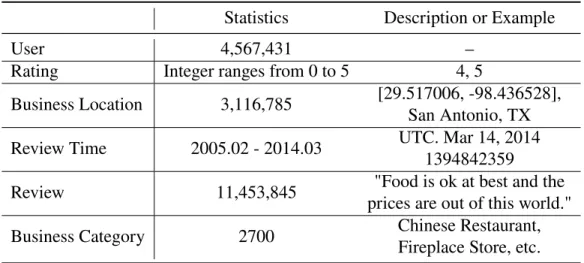
This dataset [36][?] contains a large collection of reviews about businesses from Google Local (Google Maps). Rich side information of the corresponding users and businesses is also included, such as user demographics, review time, geographic information, business opening hours and category. To be specific, geographical information contains coordinates and administrative division. Temporal information is provided in the form of both unix timestamp and GMT time. Note that this is the reviewing time rather than check-in time. The data statistics and examples are shown in Table. 3.2.
Table 3.2: Google Local Data Description and Examples
Statistics Description or Example
User 4,567,431 –
Rating Integer ranges from 0 to 5 4, 5
Business Location 3,116,785 [29.517006, -98.436528], San Antonio, TX Review Time 2005.02 - 2014.03 UTC. Mar 14, 2014
1394842359 Review 11,453,845 "Food is ok at best and the
prices are out of this world." Business Category 2700 Chinese Restaurant,
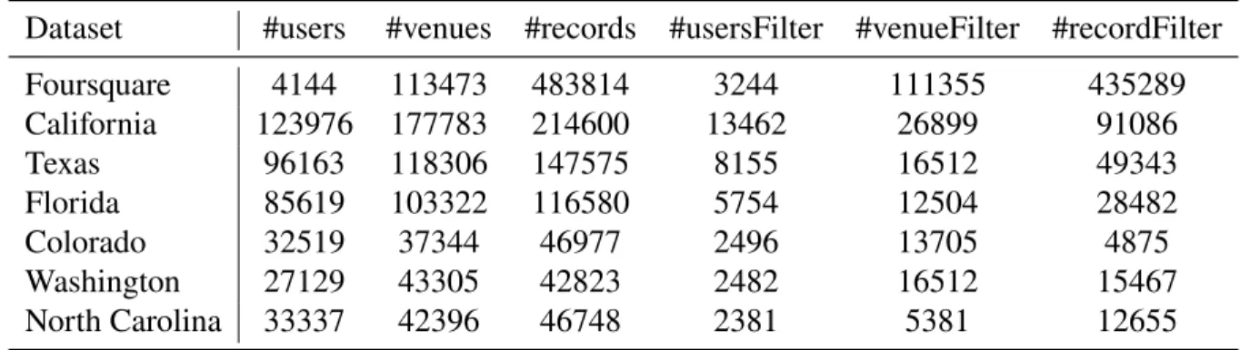
Table 3.3: Data Statistics Before and After Filtering
Dataset #users #venues #records #usersFilter #venueFilter #recordFilter Foursquare 4144 113473 483814 3244 111355 435289 California 123976 177783 214600 13462 26899 91086 Texas 96163 118306 147575 8155 16512 49343 Florida 85619 103322 116580 5754 12504 28482 Colorado 32519 37344 46977 2496 13705 4875 Washington 27129 43305 42823 2482 16512 15467 North Carolina 33337 42396 46748 2381 5381 12655
LBSNs are usually very sparse. In this work, we only use records collected from California in Foursquare dataset, and eliminate users with less than 10 check-in records in order to obtain a denser network. On Google Local dataset, we conduct experiments on data collected from six U.S. states of varying sizes and populations. Google Local dataset is even sparser than Foursquare dataset, with fewer records for each user and venue. To alleviate the effect of data sparsity, only users with more than 5 review records are kept.
The detailed dataset statistics before and after filtering are shown in Table. 3.3.
3.2
Data Characteristics and Properties
∙ Geographical Distribution
In order to get a more intuitive understanding, we visualize the geographical distribution of all venues on the state map based on venue coordinates. Figure. 3.1 and Figure. 3.2 provide the example of the geographical distribution of California venues in Foursquare and Google Local.
The visualization shows that the geographical distribution of venues from these two datasets are similar: venues are not evenly distributed across the state. The venue density of large cities such as LA county and the bay area is much higher compared with rural areas. This indicates that venue distribution is highly correlated with population distribution, and
Figure 3.1: Geographical Distribution of Foursquare Venues
Figure 3.2: Geographical Distribution of Google Local Venues
geographical information can serve as a informative indicator of the place a user may visit.
∙ Temporal Dynamics of User Mobility
Research [51][52] has shown that user mobility exhibits strong temporal cyclic patterns. Therefore, we investigate the temporal dynamics of user mobility shown in the datasets we use. Time-of-day effect and day-of-week effect are studied.
Google Local dataset only contains the time a user wrote the reviews, which is usually different from the time of visit, therefore is not suitable for studying the time-of-day effect. As a result, we only investigate this effect on Foursquare dataset, and draw the heat maps showing the types of activities users do during 12 time slots in a day, where each time slot is a 2-hour interval. Since human mobility patterns might be different during workdays and weekends, we draw two separate heat maps for workdays and weekends respectively, which are illustrated in Figure. 3.3a and Figure. 3.3b.
To study the day-of-week effect, we draw the heat map of different types of activities users do in each day of the week. We investigate this effect on both Foursquare and Google Local
dataset, which are shown in Figure. 3.4 and Figure. 3.5. For Google Local dataset, we assume that users tend to rate the business on the day of visit when memory is still fresh, and we only provide an illustration of 30 most popular business categories in California as an example.
There are several observations we can get from the illustrations:
(i). User mobility exhibits significant time-of-day effect on both workdays and weekends. For example, ’Food’ related venues are the most visited (denoted with index 11) during breakfast and dinner time, while there are only a few visits during other time of a day. (ii). Time-of-day effect is more significant than day-of-week effect. User mobility does show day-of-week effect, for example, on Foursquare, people tend to have fun at "nighttime spots" (with index 3) and go for ’Shop & Service’ (with index 26) more often during weekends, while during workdays, ’Professional & Other Places’ are more frequently visited. Google Local shows similar effect: ’American Restaurant’ (with index 26) and ’Seafood Restaurant’ (with index 10) have the largest amount of visits on Sunday. However, day-of-week effect is not as obvious compared with time-of-day effect. In fact, user mobility generally shows similar daily patterns during workdays and weekends, for example, people grab food during breakfast and dinner time, and go shopping during the night.
(iii). Among all venue categories, only a few of them are popular, which receive most of the visits. For example, on Foursquare dataset, ’Food’ and ’Shop & Service’ have 153,238 and 83,976 visits respectively, which together takes up 59% of the total check-in records. On Google Local dataset, ’American Restaurant’ takes up over 10% of the total visiting records. This effect is also clearly shown in the heat maps, as only a few activities carry bright color patch.
These observations prove that user trajectories exhibit strong temporal cyclic patterns, and suggest that (i). incorporating day-of-week effect can facilitate POI prediction task on both
(a) On Workdays (b) On Weekends
Figure 3.3: Users’ Temporal Preference for Various Activities
Figure 3.4: User Preference vs. Day-of-week on Foursquare
Figure 3.6: Sequential Patterns of User Behaviors in Foursquare
Figure 3.7: Sequential Patterns of User Behaviors in Google Local
datasets. (ii). time-of-day effect need to be considered in Foursquare dataset, while there is no need to incorporate it when studying Google Local dataset. (iii). Categorical tags are informative and can be used as a influential factor when predicting the next POI.
∙ Sequential Transition Patterns in User Trajectories
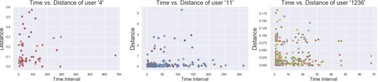
As discussed in Chapter 2, user mobility may exhibit sequential pattern. For example, users usually sequentially check-in at a restaurant, then at a cinema at weekend nights. Such sequential pattern is even more noticeable at airport and hotels. This suggests that the time interval and distance between two sequentially visited places might be highly correlated. In another word, people would only go to nearby places during a short period of time. Figure. 3.6 and Figure. 3.7 show the spatiotemporal dynamics of thee randomly picked users from Foursquare and Google Local respectively. The x-axis denotes the time interval between two sequential check-ins measured with hour, and y-axis is the distance between the two check-in venues.
Google Local. In Foursquare dataset, large time interval generally corresponds to large distance from the previous check-in spot to the current location. However, in Google Local, such pattern is not as obvious. Further inspection reveals that, the time interval between two sequential reviews in Google Local dataset is usually very large. This may due to the larger data sparsity, and users tend to give ratings and write reviews afterwards. Therefore, the sequential transitions between venues are not well reflected in Google Local dataset. The above investigation suggests that taking sequential effect into consideration can facilitate next-POI prediction on Foursquare, while might not has significant impact on Google Local.
∙ Friendship Influence
Foursquare dataset contains users’ friendship information. Friends tend to have similar preference and co-visitation behaviors. Previous work [18][19] has shown that social network can serve as auxiliary information to enhance user trajectory modeling, therefore facilitate location prediction and recommendation.
To explore the friendship influence upon user behaviors, we randomly pick 50 users in Foursquare who has social links with other users, and compare their average trajectory similarity with their friends, and all other unconnected users. Jaccard similarityis used to measure the similarity between users, which is defined as below:
𝐽(𝑢𝑖, 𝑢𝑗) = |𝑢𝑖∩𝑢𝑗|
|𝑢𝑖∪𝑢𝑗| (3.1)
where𝑢𝑖 stands for the set of venues user𝑖has visited before.
As is shown in Figure 3.8, friends visit significantly more common places. This makes sense since friends usually share similar interest, and would recommend places they have visited to each other. Co-visiting behavior is also very common. In fact, the average Jaccard Similarity among friends (0.00825) is about 5 times higher than the overall similarity
Figure 3.8: Average Jaccard Similarity Between Friends and All Users
(0.00176).
The statistical analysis further proves that friendship influence has a large impact on user behaviors, therefore can be used to facilitate location prediction and recommendation. On the other hand, similar mobility may indicate potential social links.
∙ Semantic Effect
Google Local dataset contains ratings and reviews about POIs. The semantic feedback provides valuable information which helps us make inference of the POI popularity and user preference. For example, a user gave a ’5-star’ rating to a ’Chinese restaurant’ wrote the review "Best Hot Sour soup anywhere." indicates that he has preference towards the food and is likely to visit again.
We also observe that make inference solely based on ’rating’ or ’review’ can be biased. Some users would habitually give high ratings even though they are not satisfied with the place, and vice versa. For example, a user gave a restaurant a ’3-star’ rating wrote the comment ’Sad place. Won’t be back.’, while another user gave the same rating because ’OK BUT NOT GREAT!’. This phenomena indicates that evaluating rating and review sentiment jointly will lead to a more reliable and unbiased assessment.
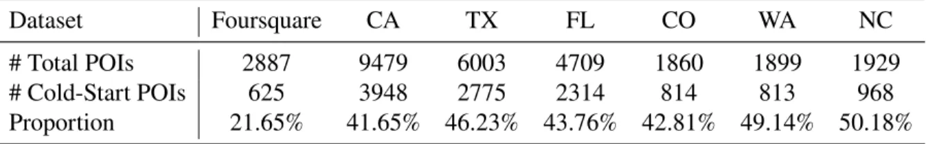
Table 3.4: Data Statistics of Cold-Start POIs
Dataset Foursquare CA TX FL CO WA NC # Total POIs 2887 9479 6003 4709 1860 1899 1929 # Cold-Start POIs 625 3948 2775 2314 814 813 968 Proportion 21.65% 41.65% 46.23% 43.76% 42.81% 49.14% 50.18%
As new places and events emerge everyday, LBSNs exhibit significant cold-start effect. In this work, since we focused on studying user mobility for user side recommendations, we only care about the influence of cold-start POIs. As will be further explained in Chapter 4, during model evaluation, we use the latest visiting record of each user as the test example. If the first appearance of a POI is in the test set, then it is considered as a cold-start POI. We count the occurrence of cold-start POIs of both datasets, the result is reported in Table. 3.4. Data statistics show that both datasets exhibit significant cold-start effect, and Google Local suffers from more severe cold-start problem compared with Foursquare dataset. In Foursquare, 21.648% of the POIs in the test set are cold-start POIs, while in Google Local, cold-start POIs take up about 45.62% of the total POIs on average.
This observation further proves that making cold-start recommendation is a non-trivial task which needs careful inspection.
Chapter 4
Methodology
4.1
Predictive Tasks
According to the analysis in Chapter 3, generally, user mobility in LBSNs exhibit six evident factors: geographical influence, temporal cyclic effect, sequential effect, semantic effect, categorical effect and friendship influence. These factors affect the spatiotemporal dynamics of user preference, therefore can be used for personalized location-based prediction. By measuring the similarity of user trajectories, we can discover users with shared behavior patterns and similar interest, thus have the potential to become friends. In addition, we have shown that enabling cold-start recommendation is a non-trivial task which needs careful inspection. In light of these observations, in this section, we define three predictive tasks we’re going to study in the following chapters.
∙ Context-aware Next-POI Prediction.
Next-POI prediction and recommendation is a most widely studied problem in LBSNs. User mobility patterns are learnt through investigating visiting history, and the rich side information about users and venues can help us understand users’ personal preference. On the other hand, unlike traditional recommendation tasks such as movie and product
recommendation, next-POI recommendation involves a more structured and context-rich environment. To be specific, besides from personal preference and mobility patterns, a rich set of context information will jointly influence a user’s choice, such as current time and location.
In this work, we study the context-aware next-POI prediction problem which takes both user preference and context information into consideration. To be specific, given a user and his or her visiting history, we make prediction on the next POI that user is likely to visit based on time and location context. We will also investigate the impact of each influential factor for a comprehensive understanding of this predictive task.
∙ Social Link Prediction and Friend Recommendation
The social network is an important part of LBSNs. Friends share their visiting experience and help us explore new places and activities. On the other hand, users can discover new friends that have shared interests with them. By comparing the personal preference and mobility patterns, we are able to measure the social distances between users and discover users with the potential to become friends.
In this work, we make effort to discover potential social links in LBSNs based on users’ shared interest and similar visiting history. A personalized friend recommendation frame-work is therefore proposed.
∙ Cold-start Recommendation
In Chapter 3, we have shown that LBSNs exhibit significant cold-start effect. In this work, we investigate the way to incorporate cold-start POIs into the recommendation framework. POI side information such as category and location can serve as auxiliary information that helps to find the potential correlation between cold-start POIs and observed POIs. In addition, the consideration of contextual features such as time and location also helps to build a robust recommender that has the ability to deal with the cold-start scenario.
4.2
Graph-based Embedding Model
Multiple factors jointly affect the predictive tasks in LBSNs. To model the interactions between these multiple factors, a graph structure turns out to be a natural choice since it is more amenable to representing and reasoning rich context compared to heuristic Factorization-based and RNN-based methods [13]. An expressive vector representation for each node in the graph needs to be found while this task is inherently difficult. A ’good’ vector representation should preserve both global structure of the graph and the local connections between nodes. In addition, the network properties and characteristics also need to be well captured.
In this work, to investigate user mobility in LBSNs, we use a bipartite graph model to depict the relations between different types of network nodes, where each type of graph links captures a certain influential factor exhibits in the network. By optimizing the first-order and second-order proximity between graph nodes, local correlations and global structure of the entire graph can be preserved. A joint training framework is proposed which embeds all the relational graphs into a shared lower-dimensional latent space.
4.2.1
Bipartite Graph Construction
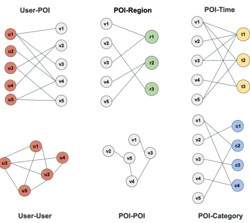
We form seven bipartite graphs to represent the relations between six types of graph nodes (POI, user, region, rating, time and category) based on the content information provided in the network. All nodes in the graphs need to be represented in a structured form. In this section, we explain how content information in the original dataset is depicted.
∙ User-POI Graph. . User-POI graph captures the interactions between users and POIs in the dataset. An edge is formed when a user visit a certain POI. It’s worth mentioning that each edge corresponds to a specific visitation, meaning there can be multiple edges between a user and a POI if the user has visited a place for multiple times. The reason we do not use a weighted edge is because the high variance of edge weights may cause gradient explosion
during optimization. More details will be covered in Section 4.2.3.
∙ POI-POI Graph. POI-POI graph captures the sequential transitions between two POIs in a user’s mobile trajectory. Note that a edge is formed only if the visiting time between two sequentially visited POIs is within a certain time interval. Like in the User-POI graph, one edge only corresponds to one transition record between two POIs.
∙ POI-Time Graph. POI-Time graph embeds the time of visit for each POI. The ’Time’ attribute is originally represented in a detailed form, which cannot be directly used as node representation. According to dataset exploration, users’ periodic mobility exhibits time-of-day and day-of-week effects. In order to encode the temporal cyclic patterns, we introduce a time-indexing strategy, which replaces the detailed temporal information with a timestamp representation. The details of the this indexing method is described as follows: (i). In Foursquare dataset, since both time-of-day and day-of-week effects exist, we denote every timestamp as a two-digit number: the first digit stands for weekdays. Monday through Sunday is represented with number 1 to 7. The second digit stands for 6 time-slots in a day, and each time-slot is a 4-hour time interval. For example, 12 am to 4 am is encoded as 0. Under this framework, a week is divided into 42 equal length time-slots.
(ii). For Google Local dataset, only day-of-week effect shows significant influence. There-fore, the timestamp is simply represented using day of week, for example, ’Monday’ and ’Friday’.
Note that each edge only corresponds to one specific visitation.
∙ POI-Region Graph. The geographical information provided in the original dataset is a combination of coordinates and administrative division, which cannot be directly used for node representations. Location coordinates are too detailed and will add enormous nodes to the network. Use city as the region unit would work fine for small counties, while is not
discriminative for large cities. Therefore, we use postcode as the region unit which has suitable scale.
∙ POI-Category GraphPOI-Category graph captures the categorical information of POIs. One POI may belong to multiple categories and there is only one edge formed between a POI and a certain category node.
∙ POI-Rating GraphGoogle Local dataset contains user ratings and reviews, which can help to make inference about POI properties and a user’s preference towards certain POIs. In addition, evaluating rating and review sentiment jointly leads to a more reliable and unbiased assessment. Therefore, we construct the POI-Rating graph to capture the semantic effect of user ratings and reviews jointly. To be specific, we compute the sentiment score for each review through sentiment analysis, then scale it to 0 5. The average of rating and the scaled sentiment score is used as the final ’rating’ value.
∙ User-User GraphUser-User graph is constructed to capture the social ties between users. Note that each social link is undirected and unweighted, for example, if user𝑢𝑖 and𝑢𝑗 are ’friends’, then the edge𝑢𝑖-𝑢𝑗 is the same as𝑢𝑗-𝑢𝑖, and will be counted only once.
To provide a more intuitive illustration of this construction strategy, Figure. 4.1 gives an example of the set of bipartite graphs built from 9 sample records, which is shown in Table 4.1.
4.2.2
Heterogeneous Graph Embedding
A graph is considered as a heterogeneous graph if two end nodes of each edge is of different types. In another word, every edge in the graph is directed.
The location network is inherently a heterogeneous graph, since each POI has different types of attributes. Therefore, we introduce a heterogeneous graph embedding strategy to embed six bipartite graphs in the location network: User-POI graph, POI-Time graph, POI-Region graph,
Table 4.1: Sample Check-in Records
Record User ID Friends Timestamp Venue ID Region ID Category ID 1 u1 u2,u3,u5 t1 v1 r1 c1 2 u1 u2,u3,u5 t2 v3 r3 c1 3 u1 u2,u3,u5 t3 v4 r1 c2 4 u2 u3,u4,u5 t1 v4 r2 c1 5 u3 u1,u2,u4,u5 t1 v2 r3 c1 6 u3 u1,u2,u4,u5 t2 v3 r2 c2 7 u4 u2,u3 t3 v2 r3 c1 8 u5 u1,u2,u3 t1 v4 r2 c1 9 u5 u1,u2,u3 t2 v5 r2 c2
POI-Rating graph, POI-Category graph and POI-POI graph. Note that the POI-POI graph is heterogeneous, since each edge is directed, pointing from one POI to the sequentially visited POI.
For heterogeneous graph embedding, we only investigate the second-order proximity between nodes. The reason is that there is no point in observing the similarity between two directly connected nodes since they’re of different types. Instead, we aim at embedding similar nodes of the same type close to each other in the embedding space, and the closeness is measured by observing the shared neighborhoods. Here, we explain the detailed embedding method:
Given a bipartite graph 𝐺𝐴𝐵 = (𝑉𝐴∪𝑉𝐵, 𝜀), where𝑉𝐴 and 𝑉𝐵 are two disjoint sets of vertices. Vertex𝑣𝑖is in𝑉𝐴and vertex𝑣𝑗 is in𝑉𝐵. Then the conditional probability of ’context’
𝑣𝑗 been generated by𝑣𝑖 is defined as:
𝑝ℎ𝑒𝑡𝑒𝑟𝑜(𝑣𝑗|𝑣𝑖) = 𝑒𝑥𝑝(𝑣⃗𝑗 𝑇 ⋅𝑣⃗𝑖) ∑ 𝑣𝑘∈𝑉𝐵𝑒𝑥𝑝(𝑣⃗𝑘 𝑇 ⋅𝑣⃗𝑖) (4.1)
The empirical distribution is computed as:
̃
𝑝ℎ𝑒𝑡𝑒𝑟𝑜(𝑣𝑗|𝑣𝑖) = 𝑤𝑖𝑗
𝑑𝑒𝑔𝑖 (4.2)
where𝑑𝑒𝑔𝑖is the degree of vertex𝑣𝑖, and𝑑𝑒𝑔𝑖=∑𝑘∈𝑁(𝑖)𝑤𝑖𝑘where𝑁(𝑖)is the set of out-neighbors of𝑣𝑖.
To preserve the second-order proximity, the conditional distribution needs to be closely ap-proximated to the empirical distribution by minimizing the distance between the two distributions, which is represented by the following objective function:
𝑂ℎ𝑒𝑡𝑒𝑟𝑜= ∑
𝑣𝑖∈𝑉𝐴
𝜆𝑖𝑑(𝑝̃ℎ𝑒𝑡𝑒𝑟𝑜(⋅|𝑣𝑖), 𝑝ℎ𝑒𝑡𝑒𝑟𝑜(⋅|𝑣𝑖)) (4.3) where𝑑(⋅,⋅)is computed using KL-divergence. 𝜆𝑖is the ’importance’ of vertex𝑣𝑖, which can be represented as the degree𝑑𝑒𝑔𝑖.
Omitting some constants, Equation. 4.3 can be calculated as:
𝑂ℎ𝑒𝑡𝑒𝑟𝑜= −∑
𝑒𝑖𝑗∈𝜀
𝑤𝑖𝑗𝑙𝑜𝑔𝑝ℎ𝑒𝑡𝑒𝑟𝑜(𝑣𝑗|𝑣𝑖) (4.4) We can obtain the embedding vectors of𝑣⃗𝑖and𝑣⃗𝑗 by minimizing Equation. 4.4
4.2.3
Homogeneous Graph Embedding
A graph is considered as a homogeneous graph if two end nodes of each edge are of the same type, and every edge in the graph is undirected.
The social network is a homogeneous graph, since User-User edge is undirected and unweighted. For homogeneous graph embedding, we only capture the first-order proximity between nodes. This makes sense for social graph embedding since users with the same neighbors make up only a small fraction of the population. The detailed embedding method is described as follows:
Given a bipartite graph 𝐺𝐴𝐵 = (𝑉𝐴∪𝑉𝐵, 𝜀), where𝑉𝐴 and 𝑉𝐵 are two disjoint sets of vertices,𝜀is the set of edges between them. Given a vertex𝑣𝑖 in𝑉𝐴and a vertex𝑣𝑗 in𝑉𝐵, the joint distribution between𝑣𝑖and𝑣𝑗 is defined as:
𝑝ℎ𝑜𝑚𝑜(�