Feature Extraction using Spiking Convolutional Neural Networks

ScholarWorks

ScholarWorks

Electrical and Computer Engineering Faculty

Publications and Presentations

Department of Electrical and Computer

Engineering

2019

Feature Extraction using Spiking Convolutional Neural Networks

Feature Extraction using Spiking Convolutional Neural Networks

Ruthvik Vaila

Boise State University

John Chiasson

Boise State University

Vishal Saxena

University of Idaho

© 2019 IEEE. Personal use of this material is permitted. Permission from IEEE must be obtained for all other uses, in any current or future media, including reprinting/republishing this material for advertising or promotional purposes, creating new collective works, for resale or redistribution to servers or lists, or reuse of any copyrighted component of this work in other works. doi: 10.1145/3354265.3354279

Feature Extraction using Spiking Convolutional

Neural Networks

Boise State University Boise, Idaho, USA

Vishal Saxena [email protected]

University of Idaho Moscow, Idaho, USA

ABSTRACT

Spiking neural networks are biologically plausible counter-parts of the artificial neural networks, artificial neural net-works are usually trained with stochastic gradient descent and spiking neural networks are trained with spike timing dependant plasticity. Training deep convolutional neural networks is a memory and power intensive job. Spiking net-works could potentially help in reducing the power usage. There is a large pool of tools for one to chose to train artificial neural networks of any size, on the other hand all the avail-able tools to simulate spiking neural networks are geared towards computational neuroscience applications and they are not suitable for real life applications. In this work we focus on implementing a spiking CNN using Tensorflow to examine behaviour of the network and study catastrophic for-getting in the spiking CNN and weight initialization problem in R-STDP using MNIST data set. We also report classifica-tion accuracies that are achieved using N-MNIST and MNIST data sets.

CCS CONCEPTS

•Computing methodologies→Machine learning; Ma-chine learning approaches;Bio-inspired approaches;

KEYWORDS

datasets, neural networks, feature extraction, STDP, R-STDP, catastrophic forgetting

1 INTRODUCTION

Deep learning, i.e., the use of deep (multi layer) convolu-tional neural networks (DCNN ), is a powerful tool for pat-tern recognition (image classification) and natural language (speech) processing [32][27]. They have been used to classify the large data set, Imagenet, [15] with an accuracy of 96.6% [1]. In this work, deep spiking networks are considered[29]. This is a new paradigm for implementing artificial neural net-works using mechanisms that incorporate spike-timing de-pendent plasticity which is a learning algorithm discovered by neuroscientists [9] [21]. The promise of spiking networks is that they are less computationally intensive and much

more energy efficient as the spiking algorithms can be imple-mented on a neuromorphic chip such as Intel’s LOIHI chip [3] (operates at low power because it runs asynchronously us-ing spikes) and other neuromorphic chips [40] [39] [41] [31]. Our work is based on the work of Masquelier and Thorpe [23] [22], and Kheradpisheh et al. [14] [13]. In particular a study is done of how such networks classify MNIST image data [17] and N-MNIST spiking data [28]. The networks used in [14] [13] consist of multiple convolution/pooling layers of spiking neurons trained using spike timing dependent plas-ticity (STDP [33]) and a final classification layer done using a support vector machine (SVM). Spike timing dependant plasticity (STDP) [20] has been shown to be able to detect hidden (in noise) patterns in spiking data [22]. Specifically, we used a simplified STDP model as in [14] given as

wi ←wi+∆wi, ∆wi =

(

+a+_{wi(1−wi), if tout−ti ≤0}

−a−_w

i(1−wi), if tout−ti >0. Heretiandtoutare the spike times of the pre-synaptic (input) and the post-synaptic (output) neuron, respectively. That is, if theith input neuron spikes before the output neu-ron spikes then the weightwi is increased otherwise the weight is decreased.1Learning refers to the change∆wi in the (synaptic) weights witha+anda−denoting the learning rate constants. These rate constants are initialized with low values(0.004,0.003)and are typically increased as learning progresses. This STDP rule is considered simplified because the amount of weight change doesn’t depend on the time duration between pre-synaptic and post-synaptic spikes.

2 BACKGROUND

In 1951 Hubel and Wiesel [10] showed that a cat’s neurons in primary visual cortex are tuned to simple features and the inner regions of the cortex combined these simple fea-tures to represent complex feafea-tures. The neocognitron model was proposed in 1980 by Fukushima to explain this behavior [8]. This model didn’t require a "teacher" (unsupervised) to learn the inherent features in the input, akin to the brain.

Knoxville ’19, July 23–25, 2019, Knoxville, TN Vaila and Chiasson, et al. The neocognitron model is a forerunner to the spiking

con-volutional neural networks considered in this work. These convolutional layers are arranged in layers to extract features in the input data. However, the deep CNNs used in industry (Google, Facebook, etc.) are fundamentally different in that they are trained using supervision (back propagation of a cost function). Here our interest is to return to the neocogni-tron model using spiking convolutional layers in which all but the output layer is trained without supervision.

Unsupervised networks

A network equipped with STDP [20] and lateral inhibition was shown to develop orientation selectivity similar to the visual frontal cortex in a cat’s brain [4]. It has been shown that deeper layers combine the features learned in the ear-lier layers in order to represent advanced features, but at the same time sparsity of the network spiking activity is maintained [14] [13] [6] [23] [37] [36] [35]. In [5] a fully connected networks trained using unsupervised STDP and homeostasis achieved a 95.6% classification accuracy on the MNIST data set.

Reward modulated STDP

Mozafari et al. [24] [25] proposed reward modulated STDP (R-STDP) to avoid using a support vector machine (SVM) as a classifier. It has been shown that the STDP learning rule can find spiking patterns embedded in noise [22]. That is, after unsupervised training, the output neuron spikes if the spiking pattern is input to it. A problem with this unsuper-vised STDP approach is that as this training proceeds the output neuron will spike when just the first few milliseconds of the pattern have been presented. Mozafari et al showed in [25] that R-STDP helps to alleviate this problem.

When unsupervised training methods are used, the fea-tures learned in the last layer are used as input to an SVM classifier [13][14] or a simple two or three layer back prop-agation classifier [34]. In contrast, R-STDP uses a reward or punishment signal (depending upon if the prediction is correct or not) to update the weights in the final layer of a multi-layer (deep) network. Spiking convolutional networks are successful in extracting features [25][13][14]. Because R-STDP is a supervised learning rule, the extracted features (reconstructed weights) more closely resemble the object they detect and thus can (e.g.,) more easily differentiate be-tween a digit “1” and a digit "7" compared to STDP. That is, reward modulated STDP seems to compensate for the inabil-ity of the STDP to differentiate between features that closely resemble each other [7] [24]. It is also reported in [24] that R-STDP is more computationally efficient. However, R-STDP is prone to over fitting, which is alleviated to some degree by scaling the rewards and punishments (e.g., receiving higher punishment for a false positive and a lower reward for a

true positive) [24] [25]. In more detail, the reward modulated STDP learning rule is:

If a reward signal is generated then the weights are up-dated according to

(

∆wij= +Nmi s s_N a+rwij(1−w_ij) iftj−ti ≤0 ∆wij=−Nmi s s

N a−rwij(1−wij) iftj−ti >0. If a punishment signal is generated then the weights are updated according to ( ∆wij =−Nhi t N a+pwij(1−wij) iftj−ti ≤0 ∆wij = +Nhi t N a−pwij(1−wij) iftj−ti >0. Heretj andti are the pre- and post-synaptic times, respec-tively. For everyNinput images,NmissandNhitare number of misclassified and correctly classified samples. Note that Nmiss+Nhit =N, if the decision of the network is based on the maximum potential of the network, if the decision of the network is based on the early spikeNmiss+Nhit ≤N because there might be no spikes for some inputs. Others have proposed error back propagation through all layers in spiking networks [18] [26], but this work focuses on using classifiers like a simple two layer back propagation, SVM, R-STDP.

Spike encoding

Spikes are either rate coded or latency coded. Rate coding refers to the information encoded by the number of spikes per second (more spikes per time carries more information) In this case the spike rate is determined by the mean rate of a Poisson process. Latency encoding refers to the information encoded in the time of arrival of a spike (earlier spikes carry more information). The spiking networks use this spatio temporal information to extract features in the input data.

Realtime spikes

Image sensors (silicon retinas) such as ATIS [30] and eDVS [2] provide (latency encoded) spikes as their output. These sensors detect changes in pixel intensities. If the pixel value at location(u,v)increases then an ON-center spike is produced while if the pixel value decreased an OFF-center spike is produced. Finally, if the pixel value does not change, no spike is produced. The spike data from an image sensor is packed using an address event representation (AER [11]) protocol and can be accessed using serial communication ports. A recorded version of spikes from eDVS sensor was introduced in [19] and a similar data set of MNIST images recorded with ATIS sensor was introduced in [28].

3 NETWORK

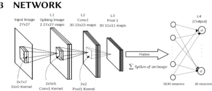
Figure 1: A deep spiking convolutional network architecture for classification of the MNIST and the N-MNIST data sets.

We have a similar network as in [14][13]. We letsL1(t,k,u,v) denote the spike signal at timetemanating from the(u,v) neuron of spiking imagekwherek =0 (ON center) ork =1 (OFF center). The L2 layers consists of 30 maps with each map having its own convolution kernel (weights) of the form WC1(w,k,i,j) ∈R2×5×5 for w =0,1,2, ...,29 (1)

The “membrane potential” of the(u,v)neuron of mapw (w =0,1,2, ...,29) of L2 at timetis given by thevalidmode convolution VL2(t,w,u,v)= t Õ τ=0 1 Õ k=0 4 Õ i=0 4 Õ i=0 sL1(τ,k,u+i,v+j)WC1(w,k,i,j) ! for(0,0) ≤ (u,v) ≤ (22,22) (2) If at timetthe potential

VL2(t,w,u,v)>γ =15 (3) then the neuron at(w,u,v)emits a unit spike.

Lateral Inhibition.To explain lateral inhibition, suppose at the location (u,v) there were potentialsVL2(t,w,u,v) in different mapsw at timet that exceeded the threshold γ Then the neuron in the map with the highest potential VL2(t,w,u,v)at(u,v)inhibits the neurons in all the other maps at the location(u,v)from spiking till the end of the present image (even if their potential exceeded the thresh-old). Figure 3 shows the accumulated spikes (from an MNIST image of “5”) from all 30 maps at each location(u,v)with lateral inhibitionnotbeing imposed. For example, at loca-tion (19,14) in Figure 3 the color code is yellow indicating in excess of 20 spikes, i.e., more than 20 of the maps produced a spike at that location.

Figure 2: Accumulation of spikes in L2withoutlateral inhi-bition. Spikes are summed across maps and time.

STDP Competition.After lateral inhibition, we consider each map that had one or more neurons whose potential V exceededγ.Let these maps bewk1,wk2, ...,wkm where2 0 ≤k1 <k2 < · · · <km ≤ 29. Then in each mapwki we locate the neuron in that map that has the maximum po-tential value. Let(uk1,vk1),(uk2,vk2), ...,(ukm,vkm)be the location of these maximum potential neurons in each map. Then neuron(uki,vki)inhibits all other neurons in mapwki from spiking for the remainder of the time steps of that spik-ing image. Further, thesemneurons can inhibit each other depending on their relative location as we now explain. Sup-pose neuron(uki,vki)of mapwkihas the highest potential of thesemneurons. Then, in an 11×11 area centered about (uki,vki),this neuron inhibits all neurons of all the other maps in the same 11×11 area. Next, suppose neuron(u_{k j},v_{k j}) of mapwk jhas the second highest potential of the remaining m−1 neurons. If the location(u_{k j},v_{k j})of this neuron was within the 11×11 area centered on neuron(u_ki,v_ki)of map wki,then it is inhibited. Otherwise, this neuron at(uk j,vk j) inhibits all neurons of all the other maps in a 11×11 area centered on it. This process is continued for the remaining m−2 neurons. In summary, there can be no more than one neuron that spikes in the same 11×11 area of all the maps. Figure 3 shows the spike accumulation after both lateral inhibition and STDP competition have been imposed. The figure shows that there is at most one spike from all the maps in any 11×11 area.

Figure 3: Accumulation of spikes with both lateral inhibi-tion and STDP competiinhibi-tion imposed. Spikes are summed across maps and time.

Max Pooling

A pooling layer is a way to down sample the spikes from the previous convolution layer to reduce the computational effort. After the synapses (convolution kernels or weights) from L1 to L2 have been learned (unsupervised STDP learn-ing is over3_{), they are fixed, but lateral inhibition continues} to be enforced in L2. Spikes from the maps of the convo-lution layer L2 are now passed on to layer L3 using max pooling. Pooling kernel is set to 2×2. Thus each map of L3 has 11×11 (down sampled) neurons. This process is repeated

2_{The other maps did not have any neurons whose membrane potential}

crossed the threshold and therefore cannot spike.

Knoxville ’19, July 23–25, 2019, Knoxville, TN Vaila and Chiasson, et al. for all the maps of L2 to obtain the corresponding maps of

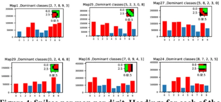
L3. Lateral inhibition is not applied in a pooling layer. There is no learning done in the pooling layer, it is just a way to decrease the amount of data to reduce the computational ef-fort. After training the L2 convolution layer, we then passed 60,000 MNIST digits through the network and recorded the spikes from the L3 pooling layer. This is shown in Figure 4. For example, in the upper left-hand corner of Figure 4 is shown the number spikes coming out of the first map of the pooling layer L3 for each of the 10 MNIST digits. It shows that the digit “3” produced over 100, 000 spikes when the 60,000 MNIST digits were passed through the network while the digit “1” produced almost no spikes. That is, the spikes coming from digit “1” do not correlate with the convolution kernel (see the inset) to produce a spike. On the other hand, the digit "3" almost certainly causes a spike in the first map of the L3 pooling layer. In the bar graphs of Figure 4 the red bars are the five MNIST digits that produced the most spikes in the L3 pooling layer while the blue bars are the five MNIST digits that produced the least.

Figure 4: Spikes per map per digit. Headings for each of the sub-plots indicate the dominant (most spiking) digit for re-spective features. This figure shows only six out of 30 maps in the L2 layer. Inset shows the feature learned by the corre-sponding map.

4 CLASSIFICATION OF MNIST DATA SETS

In the following subsections we considered a network ar-chitectures having a convolution/pool layers with different classifiers for the MNIST data set.

Classification with a Single Convolution/Pool Layer

The architecture shown in Figure 1 has a single convolu-tional/pooling layer with 30×11×11=3630 pooled neurons in L3. These neurons are fully connected to L4 layer of 3630 neurons. However, the neurons in L4 are in 1-1 correspon-dence with the L3 neurons (flatten). Further, each neuron in L4 simply sums the spikes coming into it from its correspond-ing neuron in L3. The L4 neurons are fully connected (with trainable weights) to 10 output neurons. This final layer of weights are then trained using backprop only on this output layer, i.e., only backprop to L4. The gradient of a quadratic costC =Ín0u t

i=1 (y−aL4)2gives the error from the last layer as

δL4₌ ∂C

∂aL4σ

′_(zL4_{) (4)}

aL_{is the activation of the neurons in the output layer,σis the} activation function andzis the net input to the output layer. The weights and biases of the last layer (L4) are updated as

follows: _∂C ∂bL j =δL4 j (5) ∂C ∂WL4 jk =aL3 k δjL4 (6)

(See Lee at al. [18] where the error is back propagated through all the layers and reported an accuracy of 99.3%). Inhibition settings are same as in the above experiment.The first row of Table 3 shows a 98.4% test accuracy using back propagation on the output layer (2 Layer FCN). The second and third rows give the classification accuracy using an SVM trained on the L4 neurons (their spike counts). The feature extraction that takes place in the L2 layer (and passed through the pooling layer) results in greater than 98% accuracy with a two layer conventional FCNN output classifier. A conventional FC two layer NN (i.e., no hidden layer) with the 28×28 images of the MNIST data set as input has only been reported to achieve 88% accuracy without pre-processed and 91.6% with pre-processed data [16]. This result strengthens our view that the unsupervised STDP appears to convert the MNIST classes into classes in a higher space that are separable. We also tried the same experiment in a network with two con-volution/pool layers but found that the accuracy decreased. This decrease may be due to that reduced number of spikes in the output neurons compared to have only one convolu-tion/pool layer. We then hardwired the convolution kernels of L2 layer that were trained with MNIST data set and then passed the spikes from N-MNIST data set for classification. Accuracies are reported in the Table 1. Jin et al reported an accuracy of 98.84% by using a modification of error back propagation (all layers) algorithm [12] for the N-MNIST data set. Stromatias et al reported an accuracy of 97.23% accu-racy by using artificially generated features for the kernels of the first convolutional layer and training a 3 layer fully connected neural network classifier on spikes collected at the 1st pooling layer [34] with the N-MNIST data set.

Classifier Test Acc. Val Acc. Data set 2 layer FCN 98.4% 98.5% MNIST SVM (RBF) 98.8% 98.87% MNIST SVM (linear) 98.41% 98.31% MNIST 2 layer FCN 97.45% 97.62% N-MNIST SVM (RBF) 98.32% 98.40% N-MNIST SVM (linear) 97.64% 97.71% N-MNIST Table 1: Classification accuracy on the MNIST and the N-MNIST data sets. Two layer FCN and SVM were trained on spike count vectors extracted at layer L3.

5 CATASTROPHIC FORGETTING

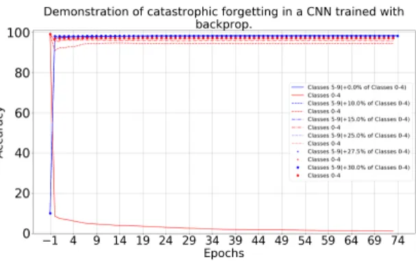
Catastrophic forgetting is a problematic issue in deep convo-lutional neural networks. In the context of the MNIST data set this refers to training the network to learn the digits 0,1,2,3,4 and, after this is done, training on the digits 5,6,7,8,9 is carried on. The catastrophic part refers to the problem that the network is no longer able to classify the first set of digits 0,1,2,3,4. A conventional (non-spiking) neural network with one convolution layer & one pool layer followed by a fully connected softmax output with only 10 outputs was first trained only on the digits 0,1,2,3,4 back propagating the error (computed from all 10 outputs) to the input (convo-lution) layer. This training used approximately 2000 digits per class and was done for 75 epochs. Before training the network on the digits 5,6,7,8,9 we initialized the weights and biases of the convolution and fully connected layer with the saved weights of the previous training. For the training with the digits 5,6,7,8,9 wefixedthe weights and biases of the convolution layer with their initial values. The network was then trained, but only the weights of fully connected layer were updated. (I.e., the error was only back propagated from the 10 output neurons to the previous layer (flattened pooled neurons). This training also used approximately 2000 digits per class and was done for 75 epochs. While the network was being trained on the second set of digits, we computed the validation accuracy on all 10 digits at the end of each epochs. We plotted these accuracies in Figure 5. The solid red line in Figure 5 are the accuracies versus epoch on the first set of digits {0,1,2,3,4} while the solid blue line gives the accuracies on the second set of digits {5,6,7,8,9} versus epoch. These plots also show the validation accuracy results when the second set of training data modified to include a fraction of data from the first set of training digits {0,1,2,3,4}. For example, the dashed red line is the validation accuracy on the first set of digits when the network was trained with 2000 digits per class of {5,6,7,8,9}along with200 (10%) digits per class of {0,1,2,3,4}. Similarly this was done with 15%, 25%, 27.5%, and 30% of the first set of digits included in the train-ing set of the second set of digits. The solid red line shows that after training with the second set of digits for a single epoch the validation accuracy on first set goes down to 10% (random accuracy). The solid blue line shows a validation accuracy of over 97% on the second set of digits after the first epoch. Thus the network has now learned the second set of digits but has catastrophically forgotten the first set of digits shown by solid red line. For more details on this topic, refer [38].

Figure 5: Catastrophic forgetting in a convolutional network while revising a fraction of the previously trained classes. Note that epoch -1 indicates that the network was tested for validation accuracy before training of the classes 5-9 started. Brackets in the legend shows the fraction of previ-ously trained classes that were used to revise the weights from the previous classes.

Forgetting In Spiking Networks

For comparison we tested forgetting in our spiking network of Section in Figure 1. The network was trained in the same fashion as we did in the non-spiking case except that STDP was used for training the L1 to L2 synapses. The solid red line in Figure 5 shows that after training with the second set of digits for a single epoch the validation accuracy on first set goes down to 77% (compared to the 10% accuracy of a non-spiking CNN). The solid blue line shows a validation accuracy of about 95% on the second set of digits after the first epoch. Thus the network has now learned the second set of digits but has not catastrophically forgotten the first set of digits shown by solid red line.

Figure 6: Catastrophic forgetting in a spiking convolutional network while revising a fraction of the previously trained classes. For more details on this topic, refer [38]

.

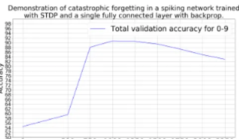
As another approach we first trained on the set {0,1,2,3,4} exactly as just describe above. However, we then took a different approach to training on the set {5,6,7,8,9}. Specifi-cally we trained on 500 random digits chosen from {5,6,7,8,9} (approximately 50 from each class) and then compute the validation accuracy on all ten digits. We repeated this for

Knoxville ’19, July 23–25, 2019, Knoxville, TN Vaila and Chiasson, et al. every additional 250 images with the results shown in Figure

7. Interestingly this shows that if we stop after training on 1000 digits from {5,6,7,8,9} we retain a validation accuracy of 91.1% and 90.71% test accuracy on all 10 digits.

Figure 7: Note that as the number of training images for the classes 5-9 increases the total accuracy drops.

6 OVER TRAINING

We used the network similar to that of in [14] [13] (by adding an extra convolution layer to the network in the Figure 1). The first row of Figure 8 shows the reconstruction of the features from the convolution kernels of the L3 to L4 layer after training with just 13500 images. In contrast, the second row of the Figure 8 shows the reconstruction of the features from the convolution kernels of the L3 to L4 layer after training with 60,000 MNIST images for 4 epochs. This shows that more training results in individual kernel weights (wij) saturating to 1 or 0 (i.e., the reconstructions in the second row are sharper), but the features become less complex. We suspect that it occurs because of STDP trying to learn the dominant first few msecs in a recurrent spatio temporal pattern.

Figure 8: Reduction in the complexity of learnt features be-cause of over training. First row of this Figure shows re-construction of L3→L4 synapses after training for 15.5k im-ages and second row shows the reconstruction of L3→L4 synapses after training for 240k images (4 epochs)

Figure 8 shows that we need a mechanism to stop training. To this end, we looked at the difference in weights during training.

W(n)

C2 ={w

(n)_{(z,i,j,k)} ∈}

R500×30×5×5 (7)

whereW_C(n₂)is kernelWC2after thenthtraining is image has passed. The L3L4 (red) plot of Figure 9 is a plot of

Í499 z=0Í29i=0Í4j=0Í4k=0 w (n∗150)_{(z,i,j,k) −w}((n+1)∗150)_(z,i,j,k) 375000 (8) for n=0,1, ...,130 (9) where 375000=500×30×5×5. Similarly the L1L2 (blue) plot was done forW_C(n₁)={w(n)(z,i,j,k)} ∈_R30×2×5×5. The L3L4 the weights dramatically change between n = 80 andn =100.Multiple experiments indicated that over training ofWC2kernels starts aftern=100. If the network was trained further, we found that the final classification accuracy drops by∼2%.

Figure 9: Plot shows the difference of successive samples of synapses, Sum(W eiдhtst−W eiдhtst−1)

no.Of.Synapses . If the difference ap-proaches zero it means that weights are not changing hence features learnt by a neuron also remain the same. Notice the sudden jump in difference between 80-100 samples. Kheradpisheh et al [14] proposed a convergence factor given by Í499 z=0 Í29 i=0 Í4 j=0Í4k=0 w (n∗150)_{(z,i,j,k)(1 −w}(n∗150)_(z,i,j,k)) 375000 (10) for n=0,1, ...,130. (11) The training was stopped when the convergence factor is between 0.01 and 0.02. We found that using this criteria there was a bit of over training resulting in 1%-2% decrease in testing accuracy.

Figure 10: Plot shows the fashion of convergence for the synapses. Note that the convergence factor dips sharply be-tween the samples 80-100.

7 WEIGHT INITIALIZATION PROBLEM IN R-STDP

MNIST data set was split into 20000 training, 40000 test and 10000 validation images. Last layer in Figure 1 was trained using R-STDP instead of simple two layer backprop. We achieved an accuracy of 90.1% on the testing data. Mozafari et al. [25][24] got around this poor performance by having 250 neurons in the output layer and assigning 25 output neurons per class. They reported 97.2 % test accuracy while

training on 60,000 images and testing on 10,000 images.We were concerned with the poor performance using an R-STDP as a classifier . In particular, perhaps the weight initialization plays a role in that the R-STDP rule can get stuck in a local minimum. To study this in more detail the network in Figure 1 was initialized with a set of weight that are known to give an accuracy of 96.8% on validation data (trained using two layer backprop). As these weights are both positive and neg-ative, they were shifted to be all positive. This was done by first finding the minimum valuewmin(<0)of these weights and simply adding−wmin >0 to them so that they are all positive. Then this new set of weights were re-scaled to be between 0 and 1 by dividing them all by their maximum value (positive). These shifted and scaled weights were then used to initialize the weights of the R-STDP classifier. The parametersa+_r,a−

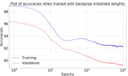
r,a+p,a−p were initialized to be 0.004, 0.003, 0.0005, 0.004 respectively. With the final layer of the network in Figure 1 initialized by these weights, further training was carried on with R-STDP.Nmiss/NandNhit/Nwere updated after every image using the most recentN images and were initialized with 0.03 and 0.97 respectively. The network was trained for 1000 epochs and the corresponding training and validation acccuracies are plotted in the Figure 11. Surpris-ingly, training and validation accuracies settled around 90%. When the same network was trained with randomly initial-ized weights fromN(0.8,0.02), training and classification accuracies increased till they reached 90% and remained con-stant. For more details on this topic, refer [38].

Figure 11: Plot of accuracies versus epochs when the weights were initialized with backprop trained weights.

8 CONCLUSION

We have studied the effects of lateral inhibition and over training in spiking convolutional networks. We reported above that using a single convolution/pool layer gives 98.4% accuracy on the MNIST data set using a two layer backprop neural network, which is a linear classifier. An accuracy of 98.8% accuracy on the MNIST data set was obtained when an SVM was used to classify the extracted features. The same experiments with the same network were carried out on the N-MNIST data set giving a 97.45% accuracy with a two layer backprop and a 98.32% accuracy using an SVM. We have demonstrated that R-STDP is sensitive to the weight initialization and a two layer error back propagation (avoids

weight transport problem) showed better performance com-pared to the R-STDP classifier. We have also shown that catastrophic forgetting is not a severe problem in spiking convolutional neural networks compared to standard (non spiking) convolution networks (The spiking network still for-gets, but not catastrophically!). Our spiking CNNs retained a total classification accuracy of 90.71% when trained on two disjoint sets and up to 95.1% when retrained using 10% of data from the previously trained data set.

ACKNOWLEDGMENTS

We would like to express our deep gratitude to Professor Timotheé Masquelier and Dr. Saeed Reza Kheradpisheh for answering our many questions about their work [14][13]. We are also grateful to Dr. Milad Mozafari for clarifying our questions about his paper [25].

REFERENCES

[1] Francois Chollet. 2017.Deep Learning with Python(1st ed.). Manning Publications Co., Greenwich, CT, USA.

[2] J. Conradt, R. Berner, M. Cook, and T. Delbruck. 2009. An embedded AER dynamic vision sensor for low-latency pole balancing. In2009 IEEE 12th International Conference on Computer Vision Workshops, ICCV Workshops. 780–785. https://doi.org/10.1109/ICCVW.2009.5457625 [3] Mike Davies, Narayan Srinivasa, Tsung-Han Lin, Gautham Chinya,

Prasad Joshi, Andrew Lines, Andreas Wild, and Hong Wang. 2018. Loihi: A Neuromorphic Manycore Processor with On-Chip Learn-ing.IEEE MicroPP (01 2018), 1–1. https://doi.org/10.1109/MM.2018. 112130359

[4] Arnaud Delorme, Laurent Perrinet, and Simon J. Thorpe. 2001. Net-works of integrate-and-fire neurons using Rank Order Coding B: Spike timing dependent plasticity and emergence of orientation selectiv-ity.Neurocomputing38-40 (2001), 539 – 545. https://doi.org/10.1016/ S0925-2312(01)00403-9 Computational Neuroscience: Trends in Re-search 2001.

[5] Peter Diehl and Matthew Cook. 2015. Unsupervised learning of digit recognition using spike-timing-dependent plasticity.Frontiers in Com-putational Neuroscience9 (2015), 99. https://doi.org/10.3389/fncom. 2015.00099

[6] Paul Ferré, Franck Mamalet, and Simon J. Thorpe. 2018. Unsupervised Feature Learning With Winner-Takes-All Based STDP. Frontiers in Computational Neuroscience12 (2018), 24. https://doi.org/10.3389/ fncom.2018.00024

[7] R˘azvan Florian. 2007. Reinforcement Learning Through Modulation of Spike-Timing-Dependent Synaptic Plasticity.Neural computation

19 (07 2007), 1468–502. https://doi.org/10.1162/neco.2007.19.6.1468 [8] Kunihiko Fukushima. 1980. Neocognitron: A self-organizing neural

network model for a mechanism of pattern recognition unaffected by shift in position.Biological Cybernetics36, 4 (01 Apr 1980), 193–202. https://doi.org/10.1007/BF00344251

[9] Demis Hassabis, Dharshan Kumaran, Christopher Summerfield, and Matthew Botvinick. 2017. Neuroscience-Inspired Artificial Intelligence.

Neuron95 (07 2017), 245–258. https://doi.org/10.1016/j.neuron.2017. 06.011

[10] D. H. Hubel and T. N. Wiesel. 1962. Receptive fields, binocular interac-tion and funcinterac-tional architecture in the cat’s visual cortex.The Journal of Physiology160, 1 (1962), 106–154. https://doi.org/10.1113/jphysiol. 1962.sp006837

Knoxville ’19, July 23–25, 2019, Knoxville, TN Vaila and Chiasson, et al.

[11] Uziel Jaramillo-Avila, Horacio Rostro-Gonzalez, Luis A. Camuňas-Mesa, Rene de Jesus Romero-Troncoso, and Bernabe Linares-Barranco. 2016. An Address Event Representation-Based Process-ing System for a Biped Robot. International Journal of Advanced Robotic Systems 13, 1 (2016), 39. https://doi.org/10.5772/62321 arXiv:https://doi.org/10.5772/62321

[12] Yingyezhe Jin, Peng Li, and Wenrui Zhang. 2018. Hybrid Macro/Micro Level Backpropagation for Training Deep Spiking Neural Networks.

arXiv-eprints(05 2018).

[13] Saeed Reza Kheradpisheh, Mohammad Ganjtabesh, and Timothée Masquelier. 2016. Bio-inspired unsupervised learning of visual features leads to robust invariant object recognition. Neurocomputing205 (2016), 382 – 392. https://doi.org/10.1016/j.neucom.2016.04.029 [14] Saeed Reza Kheradpisheh, Mohammad Ganjtabesh, Simon J. Thorpe,

and Timothée Masquelier. 2018. STDP-based spiking deep convolu-tional neural networks for object recognition. Neural Networks99 (2018), 56 – 67. https://doi.org/10.1016/j.neunet.2017.12.005 [15] Alex Krizhevsky, Ilya Sutskever, and Geoffrey E. Hinton. 2012.

Ima-geNet Classification with Deep Convolutional Neural Networks. Neu-ral Information Processing Systems25 (01 2012). https://doi.org/10. 1145/3065386

[16] Y. Lecun, L. Bottou, Y. Bengio, and P. Haffner. 1998. Gradient-based learning applied to document recognition.Proc. IEEE86, 11 (Nov 1998), 2278–2324. https://doi.org/10.1109/5.726791

[17] Yann LeCun and Corinna Cortes. 2010. MNIST handwritten digit database. http://yann.lecun.com/exdb/mnist/. (2010). http://yann. lecun.com/exdb/mnist/

[18] Chankyu Lee, Priyadarshini Panda, Gopalakrishnan Srinivasan, and Kaushik Roy. 2018. Training Deep Spiking Convolutional Neural Networks With STDP-Based Unsupervised Pre-training Followed by Supervised Fine-Tuning.Frontiers in Neuroscience12 (08 2018), 435. https://doi.org/10.3389/fnins.2018.00435

[19] Qian Liu, Garibaldi Pineda-Garc˜ıa, Evangelos Stromatias, Teresa Serrano-Gotarredona, and Steve B. Furber. 2016. Benchmarking Spike-Based Visual Recognition: A Dataset and Evaluation. Frontiers in Neuroscience10 (2016), 496. https://doi.org/10.3389/fnins.2016.00496 [20] Henry Markram, Wulfram Gerstner, and Per Jesper Sjöström. 2012. Spike-Timing-Dependent Plasticity: A Comprehensive Overview. Fron-tiers in Synaptic Neuroscience4 (2012), 2. https://doi.org/10.3389/fnsyn. 2012.00002

[21] Timothée Masquelier. 2017. Spike-based computing and learning in brains, machines, and visual systems in particular (HDR Report). Ph.D. Dissertation. https://doi.org/10.13140/RG.2.2.30232.49922

[22] Timothée Masquelier, Rudy Guyonneau, and Simon J. Thorpe. 2008. Spike Timing Dependent Plasticity Finds the Start of Repeating Pat-terns in Continuous Spike Trains. PLOS ONE3, 1 (01 2008), 1–9. https://doi.org/10.1371/journal.pone.0001377

[23] Timothée Masquelier and Simon J. Thorpe. 2007. Unsupervised Learn-ing of Visual Features through Spike TimLearn-ing Dependent Plasticity.

PLoS Computational Biology3 (2007), 1762 – 1776.

[24] Milad Mozafari, Mohammad Ganjtabesh, Abbas Nowzari, Simon Thorpe, and Timothée Masquelier. 2018. Combining STDP and Reward-Modulated STDP in Deep Convolutional Spiking Neural Networks for Digit Recognition.arXiv e-prints(03 2018).

[25] M. Mozafari, S. R. Kheradpisheh, T. Masquelier, A. Nowzari-Dalini, and M. Ganjtabesh. 2018. First-Spike-Based Visual Categorization Using Reward-Modulated STDP.IEEE Transactions on Neural Networks and Learning Systems29, 12 (Dec 2018), 6178–6190. https://doi.org/10. 1109/TNNLS.2018.2826721

[26] Emre O. Neftci, Charles Augustine, Somnath Paul, and Georgios Detorakis. 2017. Event-Driven Random Back-Propagation: Enabling Neuromorphic Deep Learning Machines.Frontiers in Neuroscience11

(2017), 324. https://doi.org/10.3389/fnins.2017.00324

[27] Michael A Nielsen. 2015. Neural Networks and Deep Learning. http: //neuralnetworksanddeeplearning.com/

[28] Garrick Orchard, Ajinkya Jayawant, Gregory K. Cohen, and Nitish Thakor. 2015. Converting Static Image Datasets to Spiking Neuromor-phic Datasets Using Saccades.Frontiers in Neuroscience9 (2015), 437. https://doi.org/10.3389/fnins.2015.00437

[29] Michael Pfeiffer and Thomas Pfeil. 2018. Deep Learning With Spiking Neurons: Opportunities and Challenges.Frontiers in Neuroscience12 (2018), 774. https://doi.org/10.3389/fnins.2018.00774

[30] C. Posch, D. Matolin, R. Wohlgenannt, M. Hofstätter, P. Schön, M. Litzenberger, D. Bauer, and H. Garn. 2010. Live demonstration: Asyn-chronous time-based image sensor (ATIS) camera with full-custom AE processor. InProceedings of 2010 IEEE International Symposium on Circuits and Systems. 1392–1392. https://doi.org/10.1109/ISCAS.2010. 5537265

[31] Vishal Saxena, Xinyu Wu, Ira Srivastava, and Kehan Zhu. 2018. To-wards Neuromorphic Learning Machines Using Emerging Memory De-vices with Brain-Like Energy Efficiency.Journal of Low Power Electron-ics and Applications8, 4 (2018). https://doi.org/10.3390/jlpea8040034 [32] J¨urgen Schmidhuber. 2015. Deep learning in neural networks: An overview. Neural Networks61 (2015), 85 – 117. https://doi.org/10. 1016/j.neunet.2014.09.003

[33] J. Sjöström and W. Gerstner. 2010. Spike-Timing Dependent Plasticity.

Scholarpedia5, 2 (2010), 1362. https://doi.org/10.4249/scholarpedia. 1362 revision #184913.

[34] Evangelos Stromatias, Miguel Soto, Teresa Serrano-Gotarredona, and Bernabé Linares-Barranco Linares-Barranco. 2017. An Event-Driven Classifier for Spiking Neural Networks Fed with Synthetic or Dynamic Vision Sensor Data. Frontiers in Neuroscience11 (2017), 350. https: //doi.org/10.3389/fnins.2017.00350

[35] Amirhossein Tavanaei, Masoud Ghodrati, Saeed Reza Kheradpisheh, Timothee Masquelier, and Anthony S. Maida. 2018. Deep Learning in Spiking Neural Networks.arXiv e-prints, Article arXiv:1804.08150 (Apr 2018), arXiv:1804.08150 pages. arXiv:cs.NE/1804.08150 [36] A. Tavanaei and A. S. Maida. 2017. Multi-layer unsupervised learning

in a spiking convolutional neural network. In2017 International Joint Conference on Neural Networks (IJCNN). 2023–2030. https://doi.org/ 10.1109/IJCNN.2017.7966099

[37] A. Tavanaei, T. Masquelier, and A. S. Maida. 2016. Acquisition of visual features through probabilistic spike-timing-dependent plasticity.2016 International Joint Conference on Neural Networks (IJCNN)(July 2016), 307–314. https://doi.org/10.1109/IJCNN.2016.7727213

[38] Ruthvik Vaila, John Chiasson, and Vishal Saxena. 2019. Deep Con-volutional Spiking Neural Networks for Image Classification.arXiv e-prints, Article arXiv:1903.12272 (Mar 2019), arXiv:1903.12272 pages. arXiv:cs.NE/1903.12272

[39] Xinyu Wu and Vishal Saxena. 2018. Dendritic-Inspired Processing Enables Bio-Plausible STDP in Compound Binary Synapses. IEEE Transactions on NanotechnologyPP (01 2018). https://doi.org/10.1109/ TNANO.2018.2871680

[40] X. Wu, V. Saxena, and K. Zhu. 2015. Homogeneous Spiking Neuro-morphic System for Real-World Pattern Recognition.IEEE Journal on Emerging and Selected Topics in Circuits and Systems5, 2 (June 2015), 254–266. https://doi.org/10.1109/JETCAS.2015.2433552

[41] X. Wu, V. Saxena, K. Zhu, and S. Balagopal. 2015. A CMOS Spiking Neuron for Brain-Inspired Neural Networks With Resistive Synapses andIn SituLearning. IEEE Transactions on Circuits and Systems II: Express Briefs62, 11 (Nov 2015), 1088–1092. https://doi.org/10.1109/ TCSII.2015.2456372