Using Markov logic for automation of mobile network management

(1)

Using Markov logic for automation of mobile

network management

Juha Niiranen

[email protected]

(2)

Faculty of Science Department of Mathematics and Statistics Juha Niiranen

Using Markov logic for automation of mobile network management Applied Mathematics

Master’s Thesis April 2016 6 + 38 p.

Mobile Network Management, Cognitive Network Management, Markov Logic Networks Kumpula Campus Library

The demand for mobile services is increasing constantly and mobile network operators need to significantly upgrade their networks to respond to the demand. The increasing complexity of the networks makes it impossible for a human operator to manage them optimally. Currently the network management operations are automated using a pre-defined logic. The future goal is to introduce cognitive network management functions which can adapt to changes in the network context and handle uncertainty in network data.

This thesis discusses using Markov Logic Networks for cognitive management of mobile networks. The method allows uncertain and partial information and makes it possible to consolidate know-ledge from multiple sources into a single, compact, representation. The model can be used to infer configuration changes in network parameters and the model parameters can be learned from data. We test the method in a simulated LTE network and examine the results in terms of improvements in network performance and computational cost.

Tiedekunta/Osasto — Fakultet/Sektion — Faculty Laitos — Institution — Department

Tekijä — Författare — Author

Työn nimi — Arbetets titel — Title

Oppiaine — Läroämne — Subject

Työn laji — Arbetets art — Level Aika — Datum — Month and year Sivumäärä — Sidoantal — Number of pages

Tiivistelmä — Referat — Abstract

Avainsanat — Nyckelord — Keywords

Säilytyspaikka — Förvaringsställe — Where deposited

(3)

Acronyms

3GPP 3rd Generation Partnership Project. BTS Base Transceiver Station.

CBR Case-Based Reasoning.

CCO Coverage and Capacity Optimisation. CLL Conditional log-likelihood.

CM Configuration management. CQI Channel Quality Indicator. FOL First-Order Logic.

IoT Internet of Things. KB Knowledge Base.

KPI Key Performance Indicator. LTE Long-Term Evolution. M2M Machine-to-Machine. MAP Maximum a Posteriori.

MCMC Markov Chain Monte Carlo. MLN Markov Logic Network.

(6)

NGMN Next Generation Mobile Networks. NMS Network Management System.

OAM Operation, Administration and Maintenance. RET Remote Electrical Tilt.

RLF Radio Link Failure.

SON Self-Organising Networks. TXP Transmission Power.

(7)

Chapter 1

Introduction

The number of mobile subscribtions in the world has increased immensely last decade. At the same time, the amount of wireless traffic continues to grow at a continuously accelerating pace. According to a recent report by Er-icsson [2], in 2014 there were 7.1 billion mobile subscriptions globally and by 2020 the number is expected to achieve 9.2 billion, of which mobile broad-band subscriptions will account for more than 80 percent. Overall mobile data traffic is expected to increase tenfold from 2014 to 2020. The report notes that the exponential growth in mobile traffic is primarily caused by the increasing demand for social networking and video streaming services. Another contributor is the emerging market of Machine-to-Machine (M2M) communications and Internet of Things (IoT) solutions.

As discussed in the book by Hämäläinen et al. [14], to cope with such massive demand for data traffic, mobile network operators need to signifi-cantly upgrade their networks and to use the resources most efficiently. This means that the networks will be very complex and the individual Network El-ements (NEs) must be dynamically configured during operation to adapt to changing traffic situations and possible malfunctions. Manual configuration of the NEs is expensive and vulnerable to mistakes. As the amount of traffic grows, the amount of money the network operators earn per transferred bit is shrinking and therefore they must try to keep their operating expenditure at the current level. This means that, in practice, configuring the individual NEs manually is impossible.

To address these challenges, the concept of Self-Organising Networks (SON) [14] has become frequently used. SON aims at increased automa-tion of network operaautoma-tions in order to utilise deployed network resources in an optimised way. Currently the SON tasks are carried out by SON func-tions in a closed-loop manner with a predefined logic. The future goal is to introduce cognitive network management functions which can learn from

(8)

data and adapt. One approach to this is to define the SON functions as knowledge-based systems, which can be automatically updated.

Handling uncertainty and contradictory information is problematic in knowledge-based reasoning. In this thesis we introduce a probabilistic sys-tem for cognitive automated network management based on Markov Logic Networks (MLNs) [22], which combines First-Order Logic (FOL) and prob-abilistic graphical models. The MLN model allows combining hypothetical information with certain domain knowledge in a single, compact, presenta-tion. MLN has been previously used in mobile network management in alarm diagnostics [6].

The structure of this thesis is as follows: in Chapter 2 we discuss mobile networks and SON in general. In Chapter 3 we go through the theory of MLN. In Chapter 4 we will introduce the MLN based network management model and in Chapter 5 we will test the model in practice. In Chapter 6 we will discuss the results and finally, in Chapter 7 we summarise and present conclusions.

(9)

Chapter 2

Mobile Networks and SON

In this chapter, we give an overview to mobile networks and their manage-ment. We also give an overview to the concept of SON, which targets the automation of management of mobile networks. Finally, we discuss the re-quirements for cognitive network management in future mobile networks.

2.1

Mobile networks overview

This overview to mobile networks has been composed from the books by Cox [7] and Schwartz [24] and the thesis by Hätönen [15]:

A mobile network provides mobile telecommunications services, such as telephone and the Internet, for a large geographical area such as a state or a country. The current state-of-the-art mobile networks are fourth generation networks, called Long-Term Evolution (LTE) networks [7]. A mobile network is run by a network operator and the network is operated via an Operation, Administration and Maintenance (OAM) system. A mobile network user can connect his or her mobile (terminal), such as a mobile phone or a tablet, to the network and move within the service area without losing the connection to the network. The continuous coverage is provided by placingbase stations

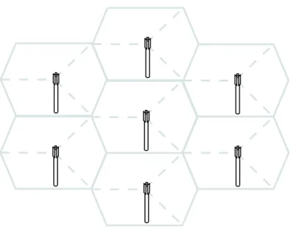
at various locations throughout the geographical area of the network. Each base station has one or more sets of antennae which are oriented to cover a sector called acell and they are used to communicate with the mobiles in the sectors. A typical base station uses three sets of antennae to control three sectors, each of which spans an arc of 120◦. Figure 2.1 shows an example layout of base stations covering a part of a mobile network.

Remark. In the remaining of this thesis we will use the word cell to refer both to a sector and to the set of antennae and other equipment in a base station that provide the coverage of the sector.

(10)

Figure 2.1: A typical BTS layout. Each BTS has three 120◦ sector cells. The size of each cell is limited by the maximum range at which the receiver can hear the transmitter. Each cell also has a limited capacity, which is determined by the maximum combined data rate of all mobiles in the cell. The required size and capacity of a cell depend on its location. There exist several types of cells with different sizes and capacities, which co-operate in a multi-layered network topology. Macrocells provide wide-range coverage in rural areas or suburbs and have a size of a few kilometres. Microcells

have a size of a few hundred metres and provide a greater collective capacity suitable for densely populated urban areas. Picocells are used in large indoor environments, such as shopping centres and offices, with a coverage area of a few tens of metres across. Finally, subscribers can buy and install home base stations in their own homes or small offices. They control femtocells, which cover an area of a few metres across.

2.2

Mobile network management

According to [11], a mobile network is managed by a Network Management System (NMS). The role of network management is to optimise the opera-tional capabilities of the network, which includes keeping the network oper-ating at peak performance. The tasks of an NMS can be divided into five categories, of which the first three are in the focus of this thesis:

(11)

• Fault management provides information on the status of the network. This includes information on failures in the network but also informa-tion on degraded performance. Fault management should be able to isolate the cause of the problem and to fix network performance.

• Configuration management is responsible for the resources to be man-aged, such as the timely deployment of network resources to satisfy expected service demand. It collects data from and delivers data for the network for the purpose of preparing for, initializing, starting, and providing for the operation and termination of services.

• Performance management is responsible for monitoring network per-formance to assure it is meeting specific goals defined by the operator. Such goals might include that sufficient capacity exists to support end-user communication requirements, but also that there is no unnecessary excess capacity and therefore no wasted resources.

• Security management controls access to the network and the NMS and protects them from abuse, unauthorised access and communication loss.

• Accounting management processes and records service and utilization information. It generates customer billing reports based on services rendered, identifies costs and establishes charges for the use of services and resources in the network.

2.3

Measurements

Network management is based on the data that the NEs, such as BTSs, generate. The NMS collects the data from the NEs for further analysis and use in different network management functions.

The data can be divided into three categories [15]:

• System configuration data contain information about how the network has been constructed and organised. These data include, among others, the network topology. These types of data are highly persistent and are not usually modified after the deployment of the network.

• System parameter data define how different system elements are imple-mented and how they operate in the network. Examples of such data include antenna transmitter output power or the threshold for the max-imum number of simultaneous connections of a BTS. These parameter data can be modified during network operation by the network opera-tor.

(12)

• Dynamic data consist of measurement values and statistical time series, alarms and other events, call records, system logs, etcetera. These data describe the dynamic use of the network and operation of processes implementing network functions.

As discussed in [18], system parameter data is handled by Configuration management (CM). Parameter changes are defined in the NMS and then deployed to NEs. For performance management, the NEs count and record all elementary events occurring during the operation of the network, forming raw low level counter value data. The time frame used in the counting depends on the management purpose and can vary from minutes to days. These counter values are analysed in order to gain information about network performance. In a typical network there exist thousands of different counters for different events, and therefore they are usually aggregated to higher level variables called Key Performance Indicators (KPIs). KPIs are formed to present understandable and easily interpretable functional factors and they are often given descriptive names.

Example 2.3.1. Here is an example of two commonly used KPIs:

1. A Radio Link Failure (RLF) [19] occurs when a user terminal inci-dentally loses the connection to the network. When the connection is re-established, the terminal can send an RLF report, indicating the last connected cell, to the network. The number of RLF events in a given time frame can then be counted for each cell.

2. An LTE terminal repeatedly sends a Channel Quality Indicator (CQI) report [7] to the BTS. The CQI report is an integer value between 0-15 and indicates maximum coding rate that the terminal can handle. The number of CQI reports in each class in a given time frame can be counted for each cell.

2.4

Self-Organising Networks (SON)

As discussed in the previous chapter, the number of adjustable settings and parameters in today’s mobile networks is too large to be addressed manually, due to the complex nature of the network, without increasing the opera-tional cost remarkably. The SON concept [14] aims at increased automation of network operations in order to utilise deployed network resources in an optimised way. Several SON use cases have been defined by the Next Gen-eration Mobile Networks (NGMN) and 3rd GenGen-eration Partnership Project

(13)

(3GPP). The SON use cases can be categorised into three functional areas [23]:

• Self-configuration consists of tasks related to bringing new NEs or NE parts to service with minimal human operator intervention. Such tasks include automatic connectivity setup between the NE and the OAM system and automatic configuration of BTS radio parameters.

• Self-optimisation consists of optimisation tasks during the operation of the network. Such tasks are needed, for example, due to changes in the network environment and are based on measurements from the network.

• Self-healing consists of actions that keep the network operational or prevent disruptive problems from arising. Such tasks include detecting faulty or degraded performance, identifying the cause for and automatic recovery from such situations.

The SON tasks are carried out by SON functions in a closed-loop manner without human intervention [31]. Typically each SON function is designed to take care of one SON use case [31].

Example 2.4.1 (Coverage and Capacity Optimisation, derived from [19]). The coverage and capacity of a cell may vary due to changes in the environ-ment. The changes can be due to season, such as trees in full leaf during summer or heavy snowfall during winter, or man-made changes in the envi-ronment. The requirements in coverage and capacity may also change due to variations in traffic distribution, for example in city centre during busy hour, if compared with quiet hours in the night. Because manual optimi-sation of network coverage and capacity is expensive and time consuming, the Coverage and Capacity Optimisation (CCO) use case has been identi-fied for automatic optimisation of network resources. One way to optimise cell capacity and coverage is to automatically adjust the Remote Electrical Tilt (RET), i.e. horizontal tilt, or the Transmission Power (TXP) of the cell antenna.

As described in [8], SON functions can operate on different levels of the network architecture. They can be located in the NMS, where they operate to meet centralized policies, reconfiguring NE parameters based on network information gathered from the NEs. They can also be located in the NEs, where they operate distributed, based on local policies received from network management.

(14)

In a self-organising system there are many SON functions which perform several tasks related to the configuration, optimisation and healing of the network. As noted by Räisänen and Tang [21], it is likely that some SON functions are applied to the same geographical area of the network at the same time. Therefore the operations of SON functions must be coordinated, so that several functions do not try to perform conflicting operations to the same area at the same time. The SON functions can be coordinated by a centralised SON coordinator, or the functions can coordinate by themselves in distributed manner [21].

Besides coordinating the operation of several SON functions, it would be beneficial that a SON system would be able to verify the activity of a SON function. After the execution of configuration change actions by a SON function, the system needs to monitor for changes in network performance. In case of undesired network behaviour caused by the actions, the system should be able to undo these configuration changes. SON verification is still under research, and not in active use [28, 29].

2.5

Cognitive network management

In a SON system the behaviour of SON functions is configured through high-level parameters and policies which are determined by a human operator according to the operational context, that is, operator goals, network en-vironment and the technical properties of the network [12]. If the context changes frequently, adapting the SON configuration can be challenging for the human operator. Because of this, the automated network management mechanisms need to be able to adapt to changes in the operational context. A report of the COMMUNE project [3] discusses the requirements and techniques for cognitive reasoning and learning in automated network man-agement. One of the requirements discussed in the report is handling uncer-tainty, i.e. coping with partial or unreliable data in the network. Another requirement discussed is the co-operation of cognitive functions deployed in different parts of the network.

One of the techniques introduced in the report is Case-Based Reasoning (CBR) [1]. In CBR experience from previous problem situations is stored into a case base and a new problem is solved by finding a similar past case and reusing the solution to the problem. In mobile network management the use of CBR has been studied especially for automatic fault detection and diagnostics [27], where a problem is expressed as a set of KPI values and a solution is either a root cause for the problem or a corrective configuration action. If there is no matching case for a problem, then a solution is acquired

(15)

from a human operator and the problem and the solution are included as a new case in the case base.

(16)

Chapter 3

Markov Logic Networks

Markov logic [22] is a language that combines first-order logic and Markov networks to define probability distributions in relational domains. In Markov logic, unlike in first-order logic, if a world violates a formula, it is not invalid, but less probable. An MLN is a first-order knowledge base with a weight attached to each formula. Other things being equal, a world that satisfies a positive (negative) weighted formula is more (less) likely than a world that does not satisfy the formula. The magnitude of the weight determines the difference of the likelihoods. An MLN can also contain hard constraints, i.e. formulas that must be satisfied for a world to be valid. Inference in Markov logic allows us to perform probabilistic reasoning over structured data.

3.1

Definition

Definition 3.1.1. A Markov logic network Lis a set of pairs (Fi,wi), where

Fi is a first-order formula and wi is a real number, the weight of formula Fi.

Together with a finite set of constants C (the constant terms to which the predicates appearing in the formulae in Lare applied to) it defines a ground Markov network ML,C as follows:

1. ML,C contains a binary node for each possible grounding of each

pred-icate appearing in the formulae of L.

2. ML,C contains one feature for each possible grounding of each formula

Fi in L.The value of the feature is 1 if the ground formula is true, and

0 otherwise. The weight of the feature is the wi associated with Fi in

L.

Remark. All features corresponding to the groundings of the same formula will have the same weight.

(17)

Remark. Hard constraints in an MLN model can be understood as formulas with infinite weights.

The set of variables X = {X1, . . . , Xn} of the ground Markov network

ML,C is thus the set of ground atoms implicitly defined by the predicates in

L and the set of constants C. The ground Markov network ML,C defines a

probability distribution over possible worlds x ∈ X, i.e. the set of possible assignments of truth values to each of the ground atoms in L, as follows,

PML,C(X =x) = 1 Z exp X i wini(x) ! (3.1) where Z :=P

x0_∈Xexp(P_iw_in_i(x0)) is the partition function andn_i(x) is the

number of the true groundings of the ith formula in possible world x ∈ X. This definition follows the log-linear representation of a Markov network.

If two possible worlds differ only on a single formulaF, then the weight of the formula is the log-odds between the two worlds. For example, ifx, x0 ∈ X, ni(x)−ni(x0) = 1 for formula Fi and nj(x) = nj(x0) for all other formulae

Fj, then PML,C(X =x) PML,C(X =x 0₎ = 1 Zexp( P kwknk(x)) 1 Zexp( P kwknk(k0)) = exp(wi(ni(x)−ni(x0))) = exp(wi)

However, usually a formulaF has common variables with other formulae, and it might not be possible to reverse the truth assignment of formula F and at the same time keep the truth assignment of those other formulae unchanged. In this situation, there is no one-to-one relation between the weights and the probabilities of the formulae.

3.2

Inference

3.2.1

MAP Inference

A basic inference task is to find the most probable state of the world given some evidence. This is known as Maximum a Posteriori (MAP) inference. From eq. (3.1) we can see that in Markov logic this reduces to finding a truth assignment that maximises the sum of the weights of the satisfied clauses. This problem can be solved using any weighted satisfiability solver. [9] efficiently use MaxWalkSAT [16], a weighted variant of the WalkSAT stochastic search satisfiability solver [25].

(18)

Algorithm 1 Network construction for inference in MLNs, adapted from [22]

Input: F1, a set of ground atoms with unknown truth value

F2, a set of ground atoms with known truth values

L, a Markov logic network

C, a set of constants

Output: M, a ground Markov network

function ConstructNetwork(F1, F2, L, C)

G←F1

while F1 6=∅ do for allq∈F1 do

if q /∈F2 then

// MB(q) is the Markov blanket of q inML,C F1 ←F1∪(MB(q)\G)

G←G∪_MB(q)

F1←F1\ {q}

return M, the ground Markov network composed of the nodes in G, all arcs between them inML,C and the weights and features on the corresponding

cliques

3.2.2

Marginal and Conditional Probabilities

Another important inference task is computing the probability that a formula holds given an MLN and a set of constants, and possibly other formulae as evidence. IfF1 andF2 are two formulae in FOL,C is a finite set of constants that includes any constants that appear in F1 orF2 and Lis an MLN, then

P(F1|F2, L, C) =P(F1|F2, ML,C) = P(F1, F2|ML,C) P(F2|ML,C) = P x∈XF₁∩XF₂PML,C(X =x) P x∈XF2 PML,C(X =x) , (3.2)

where XFi is the set of the worlds where Fi holds.

As summing over the possible worlds requires time exponential in the number of possible ground literals, computing eq. (3.2) directly is feasible only in the smallest domains. [22] propose an efficient inference algorithm for the case where F1 and F2 are conjunctions of ground literals, which, in practice, is the most common type of query. The proposed algorithm proceeds in two phases. The first phase computes the minimal subset M of the ground Markov network required to computeP(F1|F2, L, C). Pseudocode

(19)

for the first phase is shown in algorithm 1. The network is constructed as follows: First, the atoms in the query formula are added. Then, repeatedly, those atoms, that the atoms in the network depend on, and that are not in the evidence, are added, until all relevant atoms have been retrieved.

The second phase uses Gibbs sampling [5], a widespread Markov Chain Monte Carlo (MCMC) sampling technique [13], to perform inference on net-work M. The basic step consists of sampling one ground atom given its Markov blanket. The probability of a ground atom Xl when its Markov

blanket Bl is in state bl is P(Xl =xl|Bl =bl) = expP fi∈Flwifi(Xl=xl, Bl=bl) P j∈{0,1}exp P fi∈Flwifi(Xl=j, Bl =bl)

whereFlis the set of the formulae thatXlappears in, andfi(Xl=xl, Bl =bl)

is the value of the feature corresponding to the ith ground formula when Xl = xl and Bl = bl. The estimated probability of a conjunction of ground

literals is the fraction of samples where the ground literals are true, after the Markov chain has converged. Because the distribution is likely to have many modes, the Markov chain needs to be run many times. When the MLN is in clausal form, we can minimize the burn-in period by starting each round from a mode found by MaxWalkSAT.

As [10] point out, the MCMC method will not work well if the MLN contains deterministic or near-deterministic dependencies. Deterministic de-pendencies break up the space of possible worlds into regions that are not reachable from each other, which violates a basic requirement of MCMC. Near-deterministic dependencies create regions of low probabilities that are very difficult to traverse and greatly slow down inference. To solve this prob-lem, the authors in [20] introduce MC-SAT, a slice sampling algorithm, which greatly outperforms standard MCMC methods in domains with determinis-tic or near-determinisdeterminis-tic dependencies. The algorithm uses SampleSAT [33] to uniformly sample a new state.

3.3

Weight learning

The weights of the formulae in an MLN can be learned from data. Given a set of formulae and a training database of atoms, we wish to find the MAP weights of the formulae, i.e., the mode of the posterior density of the weights:

f(w|X =x) = _R Pw(X =x)f(w) Pw0(X =x)f(w0)dw0

(20)

where Pw(X = x) is the likelihood of database x given the weights w as

defined in eq. (3.1) and f(w) is the prior density of the weights. Since opti-mization is usually formulated as function miniopti-mization, we will equivalently minimize the negative posterior. The denominator of the posterior does not depend on wand can be ignored in the optimization. Thus the task of max-imising the posterior is equivalent to minimizing the sum of the negative log-likelihood and the negative log-prior:

Q(w) = −logPw(X =x)−logf(w).

A well-known method for function minimization is the gradient descent method, where we update the weight vector by taking steps proportional to the negative gradient of the function at the current point,

w(t+1) =w(t)−ηg,

where w(t−1) _{is the weight vector of the current model,} _g _{is the gradient} of function Q with respect to the current weights and η is a learning rate parameter.

The partial derivative of the log-likelihood with respect to weightwi is

∂ ∂wi logPw(X =x) = ∂ ∂wi X j wjnj(x)− ∂ ∂wi logZ =ni(x)− 1 Z ∂ ∂wi Z =ni(x)− 1 Z X x0_∈X ∂ ∂wi exp   X j wjnj(x0)   =ni(x)− 1 Z X x0_∈X exp   X j wjnj(x0)  ni(x0) =ni(x)− X x0_∈X Pw(X =x0)ni(x0),

which is the difference between the observed number of the true groundings of formula i in the data and the expected number according to the current model. As [22] point out, calculating the expected number of true groundings is intractable. Instead they propose optimizing the pseudo-likelihood of the data according to the model [4]:

P_w∗(X=x) =

n

Y

l=1

Pw(Xl=xl|M Bx(Xl)),

(21)

In many applications, the goal is to correctly predict the value of some query predicates given the value of a set of evidence predicates, and we know

a priori which predicates will be queried and which ones will be evidence. If we partition the ground atoms in the domain into a set of evidence atoms X and a set of query atoms Y, the Conditional log-likelihood (CLL) ofY given X is Pw(Y =y|X =x) = 1 Zx exp   X i∈FY wini(x, y)  ,

where FY is the set of all MLN formulae with at least one grounding

involving a query atom, ni(x, y) is the number of true groundings of the ith

formula involving query atoms and Zx is the partition function. For

simplic-ity, all non-evidence predicates are treated as query predicates. [26] show that the pseudo-likelihood method is consistently outperformed by discrim-inative training, which minimizes the CLL of the query predicates given the evidence ones. In this thesis, we will focus on discriminative training.

If we assume that the weights are independent and use a Gaussian prior for each weight wi with mean µi and variance σ2, the partial derivative of

the log-prior with respect to wi is

∂ ∂wi logf(w) = ∂ ∂wi logY j 1 √ 2πσexp − 1 2 (wj−µj)2 σ2 ! =X j ∂ ∂wi −1 2 (wj −µj)2 σ2 ! =−wi−µi σ2 .

A natural source for the prior is to use the initial formula weights as the prior means. The prior variance can then be adjusted to control the influence of the prior to the posterior distribution.

(22)

Chapter 4

MLN model for network

management

In Section 2.5 we discussed the requirements and goals for network manage-ment in future mobile networks. The main goal discussed is the ability for the network management functions to adapt to changes in the operational context. This means that, instead of operating on a static set of rules, the functions could be able to build up knowledge of the effects of the configu-ration actions. One such approach mentioned was the use of CBR in fault detection and diagnosis studied in [27]. One assumption in the article was that to each problem there is only one correct solution. In general this as-sumption is not true. As discussed in Section 2.5 the cognitive management functions need to cope with uncertainty. One source of uncertainty could be that, because it is impossible to model the network behaviour in every detail, a solution to an observable problem might work in some occurrences of the problem, but not in the others. There could also be several potential solutions to the problem.

Another requirement discussed in Section 2.5 was the co-operation of distributed cognitive functions. We would like to be able to consolidate the knowledge built up independently in the functions. If one function, for ex-ample, discovers an action that is effective in a very specific situation, we would like to make this knowledge available for other functions, perhaps op-erating in other parts of the network so that they immediately know how to act when facing this situation for the first time. Therefore we need a method of combining the Knowledge Bases (KBs) of several functions into a single model. A further motive for creating a combined model is to pro-vide a perceivable interface for the human operator to explore and to verify the discovered knowledge and possibly input and test their own hypotheses. When combining KBs of several functions (and possibly a human operator),

(23)

the resulting model may contain contradictory information.

In this chapter, we will introduce a method for cognitive network manage-ment based on MLN. Using an MLN model we are able to handle uncertain and contradictory knowledge. The model allows probabilistic inference of network configuration actions based on measured network data. We will focus on inference and learning the model parameters and assume that the (hypothetical) knowledge is acquired using external mechanisms, for example a CBR approach or from a human operator.

4.1

Model

A network management function makes changes to CM parameters based on the current status of the network, i.e. KPI values, network topology, etc. The changes are made to achieve some performance objectives, i.e. target KPI values. We will define an MLN model using these same kinds of information elements and connections between them.

4.1.1

Predicates

Our model contains three kinds of predicates:

• Context predicates indicate the current status of the network and the environment. A context predicate can indicate, for example, that some KPI value for a cell is currently below the acceptable level, that two cells are neighbours in the network topology, or that there are a lot of terminals connected to a cell. A context predicate can also indicate some properties of the current CM parameter values, for example, that the value of a parameter is at the minimum or maximum level.

• Objective predicates indicate required changes to KPI values to achieve target values defined by the operator, e.g., a particular KPI value for some cell is too low and needs to be increased.

• Action predicates indicate changes, increases or decreases, to CM pa-rameter values.

Each predicate represents an attribute of a cell in the network or a relation among the cells. The domain of a predicate can be either the set of cells X or an n-ary Cartesian product of X. For example, if predicate P represents an increase in a certain configuration parameter of a cell and predicate Q represents a neighbourship relation among a pair of cells, then the domain of P is X and the domain of Q is X×X.

(24)

To determine the values of the context predicates representing the current performance of the network, the numeric KPI values need to be categorised into ordinal classes. Defining the classification intervals of KPIs is not a straightforward task. To say that the value of a KPI is above or below normal level, one must first determine the normal level for that KPI. This is closely related to anomaly detection in mobile networks [18] and is beyond the scope of this thesis.

We assume that the acceptable region for each KPI is connected, i.e. an interval. Then we define the value of an objective predicate representing a required change to the value of a KPI as an indicator of a step towards the acceptable region of that KPI. We do not require that the acceptable region is achieved due to the step, but that the change is large enough step, i.e. larger than some predefined threshold value.

The value of an action predicate representing a change to the value of a CM parameter is defined as an indicator of a (predefined) fixed-size increase or decrease of the parameter value.

4.1.2

Formulae

We consider the knowledge in cognitive functions as a set of rules which can be expressed as a KB in FOL where each rule is a formula of the form

C1(x)∧C2(x)∧ · · · ∧Ck(x)⇒A1(x)∧A2(x)∧ · · · ∧Al(x)

which means that when the conditions indicated by the context predicates C1, C2. . . Ckhold, then CM parameter changes indicated by action predicates

A1, A2, . . . , Alare executed. This formulation is analogous to the formulation

of cases in the CBR approach discussed in Section 2.5. We assume that there exists, for each rule, a set of objective predicatesO1, O2, . . . , Om, determined

by the current performance of the network (which is indicated by the context predicates) and the KPI target values of the function. Therefore, the function rule, in effect, expresses a formula

C(x)⇒(A(x)⇒O(x)), (4.1) where C(x) = Vk

i=1Ci(x), A(x) = Vli=1Ai(x) and O(x) = Vmi=1Oi(x) are

conjunctions of the context, action and objective predicates, respectively. Although formula 4.1 is intuitively correct, it is not useful for our pur-poses: We want to use the MLN model to query for CM actions, i.e. values for the grounded action predicates. The values of the context and objective predicates are determined by the current network status and are given as ev-idence for the query. If the conjunction of the objective predicates is satisfied

(25)

by the evidence, then the formula is satisfied regardless of the values of the action predicates, and therefore the formula has no effect on the result of the query. A better alternative would be to change the direction of the right side implication of formula 4.1:

C(x)⇒(O(x)⇒A(x)). (4.2) Now, given that C(x) and O(x) are satisfied, formula 4.2 is satisfied only if also A(x) is satisfied, and the formula does affect the result of the query.

While formula 4.2 can be used for querying, it now poses another problem: If we want to learn the MLN rule weights using previous network status data, CM parameter changes and realized KPI value changes as training data, formula 4.2 is always satisfied if A(x) is satisfied, and we lose the information, whether the executed actions resulted in the wanted objectives or not. The final alternative is to use an equivalence between the object predicates and the action predicates:

C(x)⇒(O(x)⇔A(x)). (4.3) Now formula 4.3 is useful for both querying and for weight learning. For each function rule we include one such formula in the MLN model.

In addition to the formulae corresponding to the function rules, we can also include certain relational knowledge in the MLN model as hard con-straints. Such knowledge can include ontological knowledge in the telecom-munications domain or consistency constraints, such as, that the cell neigh-bourship relation is irreflexive and symmetric, that a KPI value of a cell can not both at low level and at normal level, or that a CM parameter can not be increased, if it is already at the maximum level.

Example 4.1.1. Let us look at a simple example MLN model. Let us con-sider a small network consisting of two cells: c=C1, C2, one KPI:K, and one CM parameter: P. Let us assume we know how to categorize the values of K tolow,moderateorhigh and let us define the following context predicates: IsLow(cell, K), IsM oderate(cell, K) and IsHigh(cell, K). Let us also de-fine the following objective and action predicates: ObjIncrease(cell, K), ObjDecrease(cell, K), ActIncrease(cell, P) and ActDecrease(cell, P). If our goal now is to keep the value of KPI K at a moderate level, we can

(26)

define an MLN consisting of the following formulas:

∞: IsLow(c, K)∨IsM oderate(c, K)∨IsHigh(c, K)

∞: (¬IsLow(c, K)∨ ¬IsM oderate(c, K))∧

(¬IsM oderate(c, K)∨ ¬IsHigh(c, K))∧

(¬IsLow(c, K)∨ ¬IsHigh(c, K))

∞: ¬ObjDecrease(c, K)∨ ¬ObjIncrease(c, K)

∞: ¬ActDecrease(c, P)∨ ¬ActIncrease(c, P)

w1 : IsLow(c, K)⇒(ObjIncrease(c, K)⇔ActIncrease(c, P))

w2 : IsLow(c, K)⇒(ObjIncrease(c, K)⇔ActDecrease(c, P))

w3 : IsHigh(c, K)⇒(ObjIncrease(c, K)⇔ActIncrease(c, P))

w4 : IsHigh(c, K)⇒(ObjIncrease(c, K)⇔ActDecrease(c, P)) First we have four hard constraints that guarantee that the value of K is in exactly one category and that neither the Objective nor Action can not be bothdecrease andincrease. Then we have four formulas, each of which has a real weight parameter. Now we can see that the formulas are contradictory, and the formula weights describe our belief in each formula.

4.1.3

Model composition

A function knowledge base, defined as a set of rules, can be transformed into an MLN following the procedure described in Section 4.1.2. Similarly, several functions can be transformed into a single MLN model if they share the same set of predicates. If the functions use different predicates for describing the same facts, then we need to include a mapping of the predicates. It is not reasonable to combine the knowledge bases of every function into a single model, but only of such functions that carry out related use cases.

4.2

Inference and Learning

4.2.1

Weights

The weights of the formulae in the MLN model can be learned using the method described in Section 3.3. The training data consist of observations of previous context predicate values, executed CM actions and realized ob-jectives. The initial weights given to the formulas can be used to describe our prior preferences of the rules. If we do not have any such preferences, we can initialize each weight to zero.

(27)

4.2.2

Inference

The MLN model can be used to infer CM configuration actions based on evidence. The evidence consists of context and objective predicate values which are determined by network measurements and operator targets, as discussed in Section 4.1.1. As discussed in Section 3.2, the result of the inference can be either an absolute truth value for each action (MAP state of the world) or a conditional marginal probability distribution for each action. In the latter case, the actual configuration actions can be drawn from the marginal distributions. This way we get more variance to historical data which is used as training data in the weight learning process.

(28)

Chapter 5

Experimental results

In this chapter, we study the applicability of the method introduced in the previous chapter. We will apply the MLN method to the CCO use case in-troduced in Example 2.4.1 and examine the results in terms of improvements in network performance and computational cost. We will analyse the quali-tative change in network performance as our MLN model is used to infer CM parameter changes and the model is iteratively updated based on historical data.

5.1

Setting

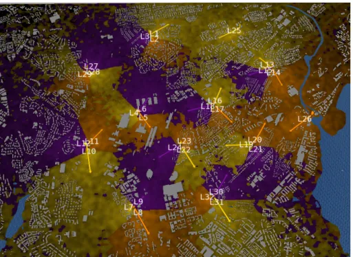
We will carry out the experiments in a simulated LTE network environment. The simulated network consists of 12 LTE macro cell base stations and 32 cells in total, covering an urban area with a size of a few kilometres across. 1000 mobile terminals move individually at random, at a walking speed, around the simulation area, so that the density of terminals is approximately the same across the whole network during the simulation. Figure 5.1 contains a screen capture of the simulation software, showing the network layout. The implementation of the simulator is based on [30].

We will try to optimise the performance of the network by adjusting the parameters of each cell simultaneously based on a single MLN model and per-formance data measured from the simulated network. The data is measured every 15 minutes and the parameter changes are made after each measure-ment round. Besides performance data, we will also use cell neighbourship information as input for the MLN model.

(29)

Figure 5.1: A screen capture of the LTE network simulator showing the network layout

5.2

Measured quantities

We will measure the following data from the network: for cell c= 1, . . . ,32, terminal u= 1, . . . ,1000 and time t >0 in minutes, let

• au,t ∈ {0,1, . . . ,32} be the cell that terminal u is connected to. If a

terminal is not connected to any cell (au,t = 0), it is outside of the

network coverage area.

• rc,t≥0 be the number of occurred RLFs (see Example 2.3.1 for details)

in cell cduring the measurement interval [t−15, t).

• dc,t = (d (0) c,t, d (1) c,t, . . . , d (15) c,t ), d (j) c,t ≥ 0, j = 0, . . . ,15, be the histogram of

CQI reports (see Example 2.3.1 for details) in each CQI class for cell c during the measurement interval [t−15, t).

We will then transform these data to the following three cell-specific scalar KPIs that are used to compute the evidence for MLN inference:

• Ac,t = P1000u=1 1c(au,t) – Number of terminals connected to a cell. We

will also compute the number of terminals that are not connected to any cell, A0,t.

(30)

• Rc,t=    0 if Ac,t= 0 rc,t Ac,t otherwise

– Ratio of occurred RLFs to the number of terminals connected to a cell.

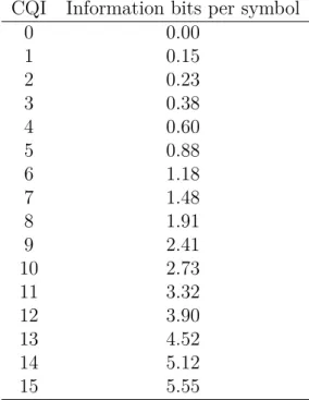
• Qc,t= P15 j=0bjd (j) c,t P15 j=0d (j) c,t

– The average channel efficiency. Herebjis the number

of information bits per transferred symbol when using the coding rate indicated by CQI class j, shown in Table 5.1.

CQI Information bits per symbol

0 0.00 1 0.15 2 0.23 3 0.38 4 0.60 5 0.88 6 1.18 7 1.48 8 1.91 9 2.41 10 2.73 11 3.32 12 3.90 13 4.52 14 5.12 15 5.55

Table 5.1: Information bits per transferred symbol for each CQI class. Adapted from [7].

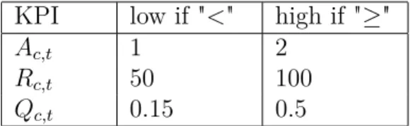
Finally, the KPI values are categorised tolow,moderate orhigh category. As discussed in the previous chapter, deciding the category limits is not a straightforward task, and the required sophisticated analysis is beyond the scope of this thesis. Instead, we will define the limits by hand. Table 5.2 shows the defined category limits. We will define our operator goals so that we wish to keep the RLF ratio Rc,t at a low level and the average channel

efficiencyQc,tat a moderate level for each cell. We will not set a target value

for the number of terminals in a cell, Ac,t, but will only use it to describe

(31)

KPI low if "<" high if "≥"

Ac,t 1 2

Rc,t 50 100

Qc,t 0.15 0.5

Table 5.2: KPI category limits for each cell cand time t.

5.3

Network parameters

We will adjust the antenna TXP and RET of the network cells. The parame-ters have an initial value, a minimum and maximum allowed value, and after each measurement round they are either increased or decreased by a fixed step size, or stay unchanged. These values are shown in Table 5.3.

Parameter init min max step size

TXP 20.0 9.0 40.0 1.0

RET 4.0 0.0 11.0 0.5

Table 5.3: Minimum and maximum values and step size of parameters for each cell.

5.4

Model

We will define an MLN model following the "Context-Objective-Action" for-mat defined in the previous chapter.

5.4.1

Variables and predicates

We will define context predicates indicating the category of each KPI value of a cell. We will also define a context predicate indicating a neighbourship relation of a pair of cells. Cells in the same BTS are always neighbours (Intra-BTS), but cells in different BTSs can also be neighbours if the cells are adjacent in the network (Inter-BTS). Finally, we will define context pred-icates indicating that a cell parameter is currently at minimum or maximum value.

We will define objective predicates indicating a desired increase or de-crease in cell KPI value for the RLF ratio Rc,t and for the average channel

efficiency Qc,t and action predicates indicating required increase or decrease

in cell parameters for TXP and RET.

The variables in the predicates are defined in Table 5.4 and the predicates are defined in Table 5.5.

(32)

Name Values Description

cell 1, . . . ,32 Cell id

kpi A, R, Q Name of the cell KPI

param RET, TXP Name of the cell parameter

nship INTER, INTRA Type of neighbourship relation

Table 5.4: Variables used in the model predicates and their possible values

Name Arguments Description

IsLow cell, kpi value of kpi of cell is at a low

level

IsMod cell, kpi value of kpiof cell is at a mod-erate level

IsHigh cell, kpi value of kpi of cell is at a high

level

IsAtMax cell, param value of param of cell is at the

maximum level

IsAtMin cell, param value of param of cell is at the

minimum level IsNeighbour cell, cell,

nship

cellis a typenshipneighbour of

cell

ObjInc cell, kpi increase value of kpi of cell

ObjDec cell, kpi decrease value of kpi of cell

ActInc cell, param increase value of param of cell

ActDec cell, param decrease value of param of cell

Table 5.5: Definition of the context, objective and action predicates used in the model.

(33)

5.4.2

Formulas and weights

As discussed in the previous chapter, we want to be able to combine knowl-edge from different sources, for example correlations discovered by cognitive network management functions and hypotheses made by a human operator. The resulting knowledge base could be large and some of the rules erroneus. Therefore we will not try to define a set of effective rules by hand. Instead, we will generate the set of formulas combinatorically from the defined context, objective and action predicates. This way we get a varied set of formulas, of which some are poor and some are good. We will generate two types of formulas as follows:

• All possible combinations of cell-specific formulas for cellcwith context predicates of one, two or three KPIs, objective predicates of one or two KPIs and action predicates of one or two parameters.

• All possible combinations of cell-pair-specific formulas for cell pair (c1, c2) with a neighbourship predicate, context predicates of one, two or three KPIs for c1, objective predicates of one or two KPIs for c1 and action predicates of one or two parameters for c2.

For both formula types we filter out those outcomes in which the objective predicates do not match the context predicates, i.e., where

• there is no context predicate for some of the KPIs of the objective predicates, or

• a context predicate indicates that an operator goal is not currently achieved, but there is no related objective predicate.

In total 1920 formulas resulted from the application of the above criteria. To make our model sound, we need to define hard constraints that guar-antee the following properties:

• A KPI value must belong to exactly one category:

(IsLow(c, k)∨IsM od(c, k)∨IsHigh(c, k))∧

(¬IsLow(c, k)∨ ¬IsM od(c, k))∧

(¬IsM od(c, k)∨ ¬IsHigh(c, k))∧

(¬IsLow(c, k)∨ ¬IsHigh(c, k))

• A KPI or a parameter value can not be both increased and decreased at the same time:

(¬ObjInc(c, k)∨ ¬ObjDec(c, k))∧

(34)

• If a parameter is currently at the maximum/minimum possible value, it can not be increased/decreased any further:

(¬IsAtM ax(c, p)∨ ¬ActInc(c, p))∧(¬IsAtM in(c, p)∨ ¬ActDec(c, p))

• The neighbourship relation is irreflexive and symmetric and two cells can not be both Inter-BTS and Intra-BTS neighbours:

(IsN eighbour(c1, c2, n)∨ ¬IsN eighbour(c2, c1, n))∧

(¬IsN eighbour(c, c, n))∧

(¬IsN eighbour(c1, c2, IN T RA)∨IsN eighbour(c1, c2, IN T ER)) The initial weights of the uncertain formulas are set to zero. The weights are updated after every 48 measurement rounds, i.e. every 12 hours, using the measurements from previous h rounds as training data.

5.5

Process

We use the Alchemy 2.0 software package [17] for MLN inference and weight learning. Alchemy 2.0 implements the marginal inference and discriminative weight learning algorithms discussed in Chapter 3.

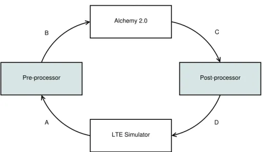
For inference, first the performance data is read from the simulator. Then the data is pre-processed together with cell neighbourship information to get truth values for all ground context and objective predicates. These values are written to a database file, which is input as evidence to infer marginal distributions for the action predicates based on the MLN model. Finally, the parameter changes are drawn from the marginal distributions and the changes are written to the simulator. This cycle is repeated every 15 minutes. Figure 5.2 shows a diagram of the inference work flow.

Remark. In the pre-processing step the objective predicate truth values are derived from the context predicate truth values based on the defined operator goals. For example, if the RLF ratio for cell 1 is high, i.e. IsHigh(1, R) is true, then also ObjDec(1, R) is true.

Remark. We draw the parameter change actions from the marginal distri-butions, so that we get variance to the data that is later used to learn the model weights, even though this could lead to suboptimal network perfor-mance. Later, when we have acquired enough data and the weights have converged, we could use the most likely action predicate values to determine corresponding network parameter changes.

(35)

Alchemy 2.0 Pre-processor LTE Simulator Post-processor A B C D

Figure 5.2: Workflow of the parameter change inference process. A: Data is read from the simulator for pre-processing. B: The pre-processed data is input to Alchemy for inference. C: Marginal distributions for action predi-cates, i.e. the output of the inference process, are used to draw parameter changes. D: The new parameter values are written to the simulator.

On each round the numerical KPI values and cell parameter values are also logged. After every 48 rounds, the model weights are updated using these data as training data. The historical sample data from the previous h rounds are pre-processed to get the realised objectives and actions. These data are then used to get a set of h database files, each of which contain the truth values of ground context, objective and action predicates for one round. These database files are input to the weight learning algorithm to get the MAP estimate weights using the current weights as prior means. Finally, the model weights are replaced by the learned MAP estimates and the new model is used for inference in the future.

5.6

Results

We will examine the changes in network performance with different history sizes h. We will try using historical data from the last 24, 48 and 96 rounds. With each history size, we run the trial for 72 hours (288 rounds), during which the model weights are updated 6 times. Forh= 96, in the first weight learning iteration we will use the data from the first 48 rounds, because there is no more data available yet. With each history size, the trial is run 3 times

(36)

and the results are averaged.

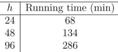
Because there are so many formulas in the model, the weight learning process would take very long to converge. Therefore we set the maximum number of gradient descent steps to 100. The algorithm always failed to converge during the maximum number of steps. Table 5.6 shows the average running times of the weight learning process1_{. We can see that the running} time is directly proportional to the history size.

h Running time (min)

24 68

48 134

96 286

Table 5.6: Average running time of the weight learning process with different history size h

Figure 5.3 shows how the total number of RLFs in the network changes as the model weights are updated with different history sizes. We can see that with all history sizes the number of RLFs begins to drop after the first update. With history sizeh= 24 the number starts to fluctuate after a couple of iterations, suggesting that 24 rounds of historical data are not sufficient for robust performance of the method. With h= 48 and h= 96 the number continues to drop after the first couple of iterations and stays stable during the rest of the iterations. The number is also substantially lower than in the beginning, where the cell parameters were set to their initial values. With h = 48 the number is most of the time slightly lower than with h = 96, so it seems that 48 rounds of historical data are enough, especially as the running time of the weight learning process doubles as the number of rounds is doubled.

Because terminals which are not connected to any cell do not generate any RLFs, we need to also examine the number of terminals which are outside the network coverage area. Figure 5.4 shows how this number changes as the model weights are updated with different history sizes. We can see that with h = 24 the situation is again unstable, but with h = 48 and h = 96 the number drops rapidly to near zero and stays low.

1_{Alchemy 2.0 was run via Cygwin on a 64-bit Windows 7 computer with a 2.70 GHz} CPU and 32 GB memory

(37)

0 500 1000 1500 2000 2500 3000 0 3 6 9 13 17 21 25 29 33 37 41 45 49 53 57 61 65 69 73

Total number of RLFs in 15 min interval

Time (h) h = 24

h = 48 h = 96 Model updated

Figure 5.3: Total number of radio link failures in the network with different history levels 0 20 40 60 80 100 0 3 6 9 13 17 21 25 29 33 37 41 45 49 53 57 61 65 69 73

Number of terminals without cell

Time (h) h = 24

h = 48 h = 96 Model updated

Figure 5.4: Total number of terminals not connected to a cell in the network with different history levels

(38)

Chapter 6

Discussion

In Chapter 4 we defined a method for consolidating knowledge from cognitive network management functions using an MLN model. In Chapter 5 we used a single MLN model for optimising an entire simulated mobile network. In a real mobile network, this would not be possible if the network management was performed in a distributed way in the NEs. However, the after the MLN model has been composed and the model weights have been fitted, the model could be disseminated back to the concerning distributed management func-tions. This approach would require that the internal knowledge presentation of the functions is implemented as an MLN.

The results in the previous chapter showed that the overall performance of the MLN model is good in the simulated network environment. One thing to consider is that the weight learning process is quite slow because of the large size of the generated model. Fortunately, the performance of the model stabilises after a few iterations, so the model weights do not have to be repeatedly updated, unless the environment changes radically or the set of formulas in the model is changed. One solution would be to try to prune the model by removing irrelevant formulas from the model. Identifying irrelevant formulas in the model requires future research.

The model that we used for experimentation is relatively simple. It only contains a couple of KPIs and parameters. In a real mobile network, the number of different measurements and parameters is much larger and all such quantities are infeasible to be included in a single model. Otherwise the size of the MLN model and the ground Markov network becomes too large very fast. Therefore the relevant measurements and parameters to be used for a particular use case need to be carefully selected. Another thing to consider is the scope of the formulas. In the previous chapter, the scope was either a single cell or a pair of cells. If the model has formulas with large scopes, the ground Markov network, again, becomes very large. Finally, in

(39)

a real environment the whole network should not be optimised together, but different parts of the network should be analysed separately.

One limitation of our MLN method is that the predicates take only boolean values. One consequence is that the KPI values need to be cate-gorised and we lose information of the magnitude of the values. Determining suitable category limits also requires sophisticated analysis, as discussed in Section 4.1.1. Another consequence is that the objectives can not be priori-tised. Each objective has equal influence on the inference even though some of them could be more critical than the others. One possible solution to this problem could be Hybrid Markov Logic Networks [32], where the real-valued functions can be used in the model together with boolean predicates.

(40)

Chapter 7

Summary and Conclusions

We presented a method for cognitive management of mobile networks using MLN. We showed that the method made it possible to combine certain and uncertain knowledge from different sources into a single, compact, represen-tation. We also showed how the model could be used for inference and how the model parameters can be learned from data. We experimented how the model performs in a simulated network environment. We also discussed the limitations of the model when applied in a real network.

The experimental results show that the model performs well in the sim-ulated environment. They show that increasing the size of historical sample data does not necessarily lead to better results, but that we get good results already with a moderate sample size. They also show that because of the large size of the generated model, the weight learning process is quite slow. In a real network setting the size of the model needs to be considered.

Possibilities for future research include reducing the model size by pruning the set of formulas and prioritising the objectives based on, for example, operator goals and the distance of the KPIs from the target values.

(41)

Bibliography

[1] Agnar Aamodt and Enric Plaza. “Case-based Reasoning: Foundational Issues, Methodological Variations, and System Approaches”. In: AI Commun. 7.1 (Mar. 1994), pp. 39–59.

[2] Ericsson AB. Ericsson Mobility Report, June 2015. http : / / www . ericsson.com/res/docs/2015/ericsson-mobility-report-june-2015.pdf. June 2015. (Visited on 04/15/2016).

[3] E. Barrett et al.Delivarable D4.1: Specification of knowledge-based rea-soning algorithms. Public Deliverable. The COMMUNE (COgnitive network ManageMent under UNcErtainty) Project (Celtic/2011-2014 CP08-004), Dec. 2012. _url: http://projects.celtic-initiative. org/commune/CELTIC_COMMUNE_D4_1_v1.pdf(visited on 04/15/2016). [4] Julian Besag. “Statistical Analysis of Non-Lattice Data”. English. In:

Journal of the Royal Statistical Society. Series D (The Statistician)

24.3 (1975), pp. 179–195.

[5] George Casella and Edward I. George. “Explaining the Gibbs Sampler”. English. In: The American Statistician 46.3 (1992), pp. 167–174. [6] Gabriela F. Ciocarlie et al. “Alarm Prioritization and Diagnosis for

Cel-lular Networks”. English. In: Mobile Networks and Management. Ed. by Ramón Agüero et al. Vol. 158. Lecture Notes of the Institute for Computer Sciences, Social Informatics and Telecommunications Engi-neering. Springer Berlin Heidelberg, 2015, pp. 28–42.

[7] C. Cox. An Introduction to LTE: LTE, LTE-Advanced, SAE and 4G Mobile Communications. Wiley, 2012.

[8] Rubén Cruz et al. In: Self-Organizing Networks (SON): Self-Planning, Self-Optimization and Self-Healing for GSM, UMTS and LTE. Ed. by Juan Ramiro and Khalid Hamied. Wiley, 2012. Chap. Multi-Technology SON.

(42)

[9] Pedro Domingos et al. “Unifying Logical and Statistical AI”. In: Proceedings of the 21st National Conference on Artificial Intelligence -Volume 1. AAAI’06. Boston, Massachusetts: AAAI Press, 2006, pp. 2– 7.

[10] Pedro Domingos et al. In: Probabilistic Inductive Logic Programming. Ed. by Luc De Raedt et al. Berlin, Heidelberg: Springer-Verlag, 2008. Chap. Markov Logic, pp. 92–117.

[11] Roger L. Freeman. Telecommunication System Engineering, 4th ed.

John Wiley & Sons, Inc., Hoboken, New Jersey, 2005.

[12] Christoph Frenzel et al. In: LTE SelfOrganising Networks (SON) -Network Management for Operational Efficiency. Ed. by Seppo Hämäläi-nen et al. Wiley, 2011. Chap. Future Research Topics.

[13] W. R. Gilks et al. Markov chain Monte Carlo in practice. London: Chapman & Hall, 1996.

[14] S. Hämäläinen et al. LTE Self-Organising Networks (SON) - Network Management for Operational Efficiency. Wiley, 2011.

[15] Kimmo Hätönen. “Data mining for telecommunications network log analysis”. PhD thesis. Helsinki, Finland: Department of Computer Sci-ence, University of Helsinki, Jan. 2009.

[16] Henry Kautz et al. “A General Stochastic Approach to Solving Prob-lems with Hard and Soft Constraints”. In: Satisfiability Problem: The-ory and Applications. American Mathematical Society, 1997, pp. 573– 586.

[17] Stanley Kok et al. The Alchemy System for Statistical Relational AI. Tech. rep. Seattle, WA: Department of Computer Science and En-gineering, University of Washington. _url: http : / / alchemy . cs . washington.edu.

[18] Pekka Kumpulainen. “Anomaly Detection for Communication Network Monitoring Applications”. PhD thesis. Tampere, Finland: Department of Automation Science and Engineering, Tampere University of Tech-nology, Mar. 2014.

[19] Daniela Laselva et al. In: LTE Self-Organising Networks (SON) - Net-work Management for Operational Efficiency. Ed. by Seppo Hämäläi-nen et al. Wiley, 2011. Chap. Self-Optimisation.

(43)

[20] Hoifung Poon and Pedro Domingos. “Sound and Efficient Inference with Probabilistic and Deterministic Dependencies”. In: Proceedings of the 21st National Conference on Artificial Intelligence - Volume 1. AAAI’06. Boston, Massachusetts: AAAI Press, 2006, pp. 458–463. [21] Vilho Räisänen and Haitao Tang. “Knowledge Modeling for Conflict

Detection in Self-organized Networks”. English. In: Mobile Networks and Management. Ed. by Kostas Pentikousis et al. Vol. 97. Lecture Notes of the Institute for Computer Sciences, Social Informatics and Telecommunications Engineering. Springer Berlin Heidelberg, 2012, pp. 107– 119.

[22] Matthew Richardson and Pedro Domingos. “Markov Logic Networks”. In: Machine Learning 62.1-2 (Feb. 2006), pp. 107–136.

[23] Cinzia Sartori et al. In: LTE Self-Organising Networks (SON) - Net-work Management for Operational Efficiency. Ed. by Seppo Hämäläi-nen et al. Wiley, 2011. Chap. Introduction.

[24] M. Schwartz. Mobile Wireless Communications. Cambridge University Press, 2005.

[25] Bart Selman et al. “Local Search Strategies for Satisfiability Testing”. In: Cliques, Coloring, and Satisfiability: Second DIMACS Implemen-tation Challenge, October 11-13, 1993. Ed. by David S. Johnson and Michael A. Trick. Center for Discrete Mathematics and Theoretical Computer Science New Brunswick, NJ: DIMACS series in discrete mathematics and theoretical computer science. American Mathemati-cal Society, 1996, pp. 521–532.

[26] Parag Singla and Pedro Domingos. “Discriminative Training of Markov Logic Networks”. In: Proceedings of the 20th National Conference on Artificial Intelligence - Volume 2. AAAI’05. Pittsburgh, Pennsylvania: AAAI Press, 2005, pp. 868–873.

[27] P. Szilágyi and S. Nováczki. “An Automatic Detection and Diagno-sis Framework for Mobile Communication Systems”. In: Network and Service Management, IEEE Transactions on 9.2 (June 2012), pp. 184– 197.

[28] Tsvetko Tsvetkov et al. “A Post-Action Verification Approach for Auto-matic Configuration Parameter Changes in Self-Organizing Networks”. English. In:Mobile Networks and Management. Ed. by Ramón Agüero et al. Vol. 141. Lecture Notes of the Institute for Computer Sciences, Social Informatics and Telecommunications Engineering. Springer In-ternational Publishing, 2015, pp. 135–148.

(44)

[29] T. Tsvetkov et al. “A configuration management assessment method for SON verification”. In:Wireless Communications Systems (ISWCS), 2014 11th International Symposium on. Aug. 2014, pp. 380–384. [30] I. Viering et al. “A Mathematical Perspective of Self-Optimizing

Wire-less Networks”. In: Communications, 2009. ICC ’09. IEEE Interna-tional Conference on. June 2009, pp. 1–6.

[31] Richard Waldhauser et al. In: LTE SelfOrganising Networks (SON) -Network Management for Operational Efficiency. Ed. by Seppo Hämäläi-nen et al. Wiley, 2011. Chap. Self-Organisin