Support Vector Machine and Its Application to Regression and Classification

BearWorks

BearWorks

MSU Graduate Theses

Spring 2017

Support Vector Machine and Its Application to Regression and

Support Vector Machine and Its Application to Regression and

Classification

Classification

As with any intellectual project, the content and views expressed in this thesis may be considered objectionable by some readers. However, this student-scholar’s work has been judged to have academic value by the student’s thesis committee members trained in the discipline. The content and views expressed in this thesis are those of the student-scholar and are not endorsed by Missouri State University, its Graduate College, or its employees.

Follow this and additional works at: https://bearworks.missouristate.edu/theses

Part of the Mathematics Commons

Recommended Citation Recommended Citation

Hu, Xiaotong, "Support Vector Machine and Its Application to Regression and Classification" (2017). MSU Graduate Theses. 3177.

https://bearworks.missouristate.edu/theses/3177

This article or document was made available through BearWorks, the institutional repository of Missouri State University. The work contained in it may be protected by copyright and require permission of the copyright holder for reuse or redistribution.

SUPPORT VECTOR MACHINE AND ITS APPLICATION TO REGRESSION AND CLASSIFICATION

A Masters Thesis Presented to The Graduate College of Missouri State University

In Partial Fulfillment

Of the Requirements for the Degree Master of Science, Mathematics

By Xiaotong Hu

SUPPORT VECTOR MACHINE AND ITS APPLICATION TO REGRESSION AND CLASSIFICATION

Mathematics

Missouri State University, April 2017 Master of Science

Xiaotong Hu

ABSTRACT

Support Vector machine is currently a hot topic in the statistical learning area and is now widely used in data classification and regression modeling. In this thesis, we introduce the basic idea for support vector machine, its application in the classification area including both linear and nonlinear parts, and the idea of support vector regression contains the comparison of loss functions and the usage of kernel function. Two real life examples, which are taken from R package, are also provided for both classification and regression part respectively, talking about classification of glass type and prediction for Ozone pollution.

KEYWORDS: support vector machine, data Classification, regression model, hyperplane, statistical learning

This abstract is approved as to form and content

_______________________________ Songfeng Zheng, PhD

Chairperson, Advisory Committee Missouri State University

SUPPORT VECTOR MACHINE AND ITS APPLICATION TO REGRESSION AND CLASSIFICATION

By Xiaotong Hu A Master Thesis

Submitted to the Graduate College Of Missouri State University In Partial Fulfillment of the Requirements For the Degree of Master of Science, Mathematics

May, 2017 Approved: _________________________________ Songfeng Zheng, PhD _________________________________ Yingcai Su, PhD _________________________________ George Mathew, PhD _________________________________ Julie Masterson, PhD: Dean, Graduate College

TABLE OF CONTENTS

Chapter 1. Introduction ...1

1.1 Basic Idea of Statistical Learning Theory...1

1.2 Introduction to Support Vector Machine ...1

Chapter 2. Support Vector Classification ...3

2.1 Hyperplane...3

2.2 Maximal Margin Classifier ...3

2.2.1 Classification using a Separating Hyperplane ...3

2.2.2 The Maximal Margin Classifier...4

2.3 Support Vector Classifier...6

2.3.1 Overview of Support Vector Classifier...6

2.3.2 Computing the Support Vector Classifier...8

2.4 Classification with non-linear decision boundaries ...11

2.5 Application of Support Vector Classification to Real World Data...13

Chapter 3. Support Vector Regression...23

3.1 Linear regression...23

3.1.1 ε-insensitive Loss Function...23

3.1.2 Quadratic Loss Function ...27

3.1.3 Huber Loss Function...28

2.3 Nonlinear Regression...30

2.5 Application of Support Vector Regression to Real World Data...32

References...39

Appendices ...40

Appendix A. Glass Data ...40

LIST OF TABLES

Table 1. Different Type of Glass and their Chemical Analysis Data (Partial) ...12

Table 2. Summary of Data ‘Glass’ ...13

Table 3. Quantities for Each Type of Glass...13

Table 4. Summary of Base Model for Data ‘Glass’...15

Table 5. Statistics of Base Model for Data ‘Glass’...16

Table 6. Summary of Adjusted Model 1 for Data ‘Glass’...17

Table 7. Statistics of Adjusted Model 1 for Data ‘Glass’ ...18

Table 8. Summary of Adjusted Model 2 for Data ‘Glass’...18

Table 9. Statistics of Adjusted Model 2 for Data ‘Glass’ ...19

Table 10. Summary of Fittest Model for Data ‘Glass’ ...20

Table 11. Statistics of Fittest Model for Data ‘Glass’ ...21

Table 12. Los Angeles daily ozone pollution in 1976 (Partial) ...33

Table 13. Summary of Base Model for Data ‘Glass’...35

Table 14. Summary of Adjusted Model 1 for Data ‘Glass’...36

Table 15. Summary of Adjusted Model 2 for Data ‘Glass’...37

LIST OF FIGURES

Figure 2.1 Separating Hyperplane 𝛽0+𝛽1𝑥1+𝛽2𝑥2=0 in 2-dimensional space...4

Figure 2.2 Maximal Margin Classifier and the margin in 2-dimisional space ...5

Figure 2.3 Hyperplane change leaded by a single observation...7

Figure 2.4 Soft Margin Classifier ...7

Figure 2.5 Support Vector Machine with polynomial kernel of degree 3 ...12

Figure 3.1 A plot of typical ε-insensitive loss function ...24

Figure 3.2 A plot of typical quadratic loss function ...27

Figure 3.3 Huber loss and quadratic loss as a function of𝑦 ‒ 𝑓(𝑥)...29

CHAPTER 1. INTRODUCTION 1.1 Basic Idea of Statistical Learning Theory

Statistical learning theory is a framework for machine learning area related to the fields of statistics and functional analysis. The goal for statistical learning is find a fittest function , representing the systematic information of the response from its predictors, 𝑓 which will be used for prediction and inference.

To estimate this unknown function, the approach used in statistical learning is called training data, whose name come from the usage that train our method how to estimate . Every point in the training data is a input-output pair, where the input maps an 𝑓 output. The statistical leaning problem consist of inferring the function that maps

between the input and the output, such that the learned function can be used to predict output from future input.

Statistical learning theory is widely used in regression modeling and data

classification. In the regression problem, the responses are quantitative values which take a continuous range of values, meanwhile, the responses in classification problem are qualitative values which are elements from a discrete set of labels. In the statistical learning area, the approach to find the function are different in many aspects, for 𝑓 example, the choice of loss function, however, they also share some similarities. In the following chapter, we will go further in both of these two areas.

1.2 Introduction to Support Vector Machine

Support Vector machine are currently a hot topic in the statistical learning area. In late 1990s, the traditional neural network approaches suffered severe difficulties with generalization and producing models which is the main reason for the foundation of

support vector machines. It was developed in 1995 by Vladimir Vapnik, and soon gained popularity due to many attractive features.

In statistical learning, support vector machines are supervised learning method with assoxiated leaning algorithms that analyze dataset. It is first been introduced as an method for solving classification problems. However, due to many attractive features, it is recently extended to the area of regression analysis.

This thesis will mainly focus on the application of support vector machine used in classification and regression area and is structured as follows.

Chapter 2 introduces the basic idea of classification, including the concept of hyperplane, different type of classifier and their properties, and will be focused on the support vector classification in both linear and non-linear condition, and its application in real life examples operating by computational languages R.

Chapter 3 will focus on support vector regression which is separated into linear and non-linear regression. In both these two sections, it will introduce different type and choice for loss function and how will it influence the performance of regression

modeling. It will also introduce an example at the end of these chapter to show how support vector regression deals with real life problem.

CHAPTER 2. SUPPORT VECTOR CLASSIFICATION 2.1 Hyperplane

In a p-dimensional space, a hyperplane is a flat affine subspace (a subspace need not pass through the origin) of dimension p-1. It is defined by equation

(2.1) 𝛽₀+𝛽₁𝑥₁+𝛽₂𝑥₂+ … +𝛽_𝑝𝑥_𝑝= 0

for parameter 𝛽1…𝛽𝑝. In this case, the point X=(𝑥1,𝑥2,…,𝑥𝑝) lies on the hyperplane.

Now, suppose X does not satisfy 2.1, but

𝛽₀+𝛽₁𝑥₁+𝛽₂𝑥₂+ … +𝛽_𝑝𝑥_𝑝> 0 (2.2)

then we say X lies on the one side of the hyperplane. On the other hand, if 𝛽₀+𝛽₁𝑥₁+𝛽₂𝑥₂+ … +𝛽_𝑝𝑥_𝑝< 0 (2.3)

then X lies on the other side of the hyperplane.

Here we can consider that the hyperplane divides this p-dimensional space into two halves, which will be the basic idea of classification.

2.2 Maximal Margin Classifier

2.2.1 Classification using a Separating Hyperplane

Suppose we have a 𝑛×𝑝 data matrix that contains n observation in p-dimensional space 𝑥₁=

(

)

(

)

What we want is to separate these data into two class. The approach is to label , where -1 represent a class and 1 represent the other class. Our goal is 𝑦₁,…,𝑦_𝑛∈{‒1,1}

it is based on the concept of separating hyperplane (James, Witten, Hastie & Tibshirani, 2009).

The separating hyperplane with parameter 𝛽1…𝛽𝑝 has the property that

{

𝛽₀+𝛽₁𝑥_{𝑖 1}+𝛽₂𝑥_{𝑖 2}+ … +𝛽_𝑝𝑥_{𝑖 𝑝}<0, 𝑖𝑓 𝑦_𝑖=‒1 (2.4)

which equivalently means

𝑦_𝑖(𝛽₀+𝛽₁𝑥₁+𝛽₂𝑥₂+ … +𝛽_𝑝𝑥_𝑝) > 0 (2.5)

Thus, if a hyperplane exist, the observation dataset can be assigned a class based on which side if the hyperplane it is located. In figure 2.1, we can clearly classify the observation based on hyperplane 𝑥𝑖 𝛽0+𝛽1𝑥1+𝛽2𝑥2=0. That is, if

is positive, it is assigned to class 1; if negative, on the other 𝑓

(

)

Figure 2.1 Separating Hyperplane 𝛽0+𝛽1𝑥1+𝛽2𝑥2=0 in 2-dimensional space 2.2.2 The Maximal Margin Classifier

In general, if our data can be perfectly separated using a hyperplane, then there will exist infinitely many such hyperplane. In order to decide which separating

hyperplane to use, we need to use the maximal margin classifier, which is also known as the optimal separating hyperplane. The maximal margin classifier is farthest from the training observation. That is, when we compute the distance of each observation to the separating hyperplane, the minimal one is what we called ‘the margin’. The maximal margin classifier is the hyperplane for which the margin is the largest (James, Witten, Hastie & Tibshirani, 2009).

In general, the maximal margin classifier is the solution to the optimization problem max 𝛽₀,𝛽₁,…,𝛽_𝑝𝑀 (2.6) 𝑠𝑢𝑏𝑗𝑒𝑐𝑡 𝑡𝑜 𝑝

∑

Equation 2.5 guarantees M is positive, and with constraints from 2.6 to 2.8, the perpendicular distance for th observation to the hyperplane is actually given by 𝑖

. Thus, M is the margin of the hyperplane, and the 𝑦_𝑖(𝛽₀+𝛽₁𝑥₁+𝛽₂𝑥₂+ … +𝛽_𝑝𝑥_𝑝)

optimization problem is exactly the definition of the maximal margin hyperplane. 2.3 Support Vector Classifier

2.3.1 Overview of Support vector Classifier

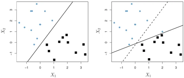
Sometimes in practical situation, the observations that belong to two classes are not necessarily separable by the hyperplane. In fact, the maximal margin hyperplane may not be desirable even if it does exist. A classifier based on the maximal margin

hyperplane could be changed dramatically with addition or miss one single observation which may result in overfitting the training data. An example is shown in figure 2.3, where a single observation could dramatically change the hyperplane from the left-handle panel to the right handle panel.

Figure 2.3 Hyperplane change leaded by a single observation

In this case, another approach to classify the observation, which is known as soft margin classifier or support vector classifier is needed. Unlike maximal margin classifier, the soft margin classifier allows some observation on the wrong side of the margin or even on the wrong side of the hyperplane.

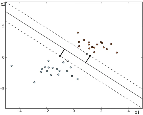
Figure 2.4 shows an example of soft margin classifier. Here, observation x1 is on the wrong side of margin but right side of hyperplane, and observation x2 is on both wrong side of margin and hyperplane. Observation x3, 4 and 5, which lie on the edge of the margin, these 3 observations and observation x1 and x2 which lie inside the soft margin are what we called ‘the support vectors’, and we will detail this part in 2.3.2. Similar with the maximal margin classifier, the soft margin classifier is the solution to the optimization problem

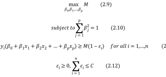
max 𝛽₀,𝛽₁,…,𝛽_𝑝𝑀 (2.9) 𝑠𝑢𝑏𝑗𝑒𝑐𝑡 𝑡𝑜 𝑝

∑

∑

where C is a nonnegative tuning parameter. As showing in Figure 2.3, M is the width of the margin, which we seek to make this value as large as possible. is what we called ‘ 𝜀𝑖

slack variables’ that allows individual observation to be on the wrong side of margin or hyperplane. By the constraints shows from 2.9 to 2.11, we can easily tell that if

, the observation is on the wrong side of margin but right side of hyperplane (

0≤ 𝜀_𝑖≤1

in Figure 2.3 with slack variable ); if , the observation is on the both wrong

𝑥₁ 𝜀₁ 𝜀_𝑖≥1

side of margin and hyperplane ( in Figure 2.3 with slack variable ) .𝑥2 𝜀2

2.3.2 Computing the Support Vector Classifier We can rewrite 2.9-2.12 into

max 𝛽,𝛽_{0,||𝛽|| = 1}𝑀 (2.13) 𝑦_𝑖(𝑥𝑇_𝑖𝛽+𝛽₀)≥ 𝑀(1 ‒ 𝜀_𝑖) 𝑓𝑜𝑟 𝑎𝑙𝑙 𝑖=1,…,𝑛 (2.14) 𝜀_𝑖≥0, 𝑛

∑

where 𝑥𝑖∈ 𝑅𝑝 with unit vector ||𝛽|| = 1. If we then drop the norm constraint on , where 𝛽

we define 𝑀= 1/||𝛽||, 2.13-2.15 will be represented as

(2.16) 𝑚𝑖𝑛⁡||𝛽|| subject to 𝑦𝑖(𝑥𝑇𝑖𝛽+𝛽0)≥1‒ 𝜀𝑖 𝑓𝑜𝑟 𝑎𝑙𝑙 𝑖=1,…,𝑛 (2.17) 𝜀_𝑖≥0, 𝑛

∑

The problem 2.16-2.18 is a quadratic with linear inequality constraints, hence, we can describe the programming solution using Lagrange multipliers (Smola & Scholkopf, 2003). The problem is equivalent to

min1 2||𝛽|| 2 +𝐶 𝑛

∑

The Lagrange function is 𝐿=1 2||𝛽|| 2 +𝐶 𝑛

∑

∑

[

)

∑

𝛽= 𝑁

∑

∑

where the constraints 𝛼𝑖,𝜇𝑖,𝜀𝑖≥0. By substituting 2.23-2.25 into 2.22

max𝐿= 𝑁

∑

∑

∑

∑

In addition, the Karush-Kuhn-Trcker conditions that are satisfied by the solution are, (2.29) 𝛼_𝑖

[

)

[

)

For 𝑖=1,…𝑁. All the equations from 2.23-2.29 uniquely characterize the solution to the primal and dual problems (Smola & Scholkopf, 2003).

Meanwhile, from 2.23, we can get the solution for β which is in the form of , and the observations with constraints in 2.31 are what we called support 𝛽=∑𝑁_{𝑖= 1}𝛼_𝑖𝑦_𝑖𝑥_𝑖

vectors, some meet the constrains in 2.29, which are observations lies on the edge of the margin, and we normally use them to solve 𝛽0.

2.4 Classification with Nonlinear Decision Boundaries

In general, the soft margin classifier is a approach for linear boundary

classification. However, we sometimes need to deal with nonlinear boundary in practice when linear classifier cannot perfectly perform. In this case, we need to enlarge the feature space using functions of predictors, like quadratic or cubic. For example, with p observation 𝑥1,…𝑥𝑝, we can fit a vector classifier along with their quadratic form, i.e.

Thus, the optimization problem show from 2.9 to 2.12 will become 𝑥₁, 𝑥2₁,…,𝑥_𝑝,𝑥2_𝑝. max 𝛽₀,𝛽₁₁,…,𝛽_𝑝1,𝛽₁₂,…𝛽_𝑝2𝑀 (2.32) 𝑠𝑢𝑏𝑗𝑒𝑐𝑡 𝑡𝑜 𝑝

∑

∑

∑

∑

∑

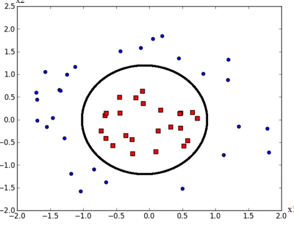
The solution will lead to a nonlinear decision boundary, which is known as support vector machine.

The key idea of support vector machine is what we called the kernel (James, Witten, Hastie & Tibshirani, 2009). A kernel is a function which quantifies the similarity

of two observation, representing as 𝐾(𝑥𝑖,𝑥𝑖'). For example, we can represent linear

support vector classifier by taking inner product as kernel, which means 𝐾

(

)

∑

and the support vector classifier can be represented as 𝑓(𝑥) =𝛽₀+ 𝑝

∑

(

)

which is also the general form of support vector machine if 𝐾(𝑥𝑖,𝑥𝑖') is not specific. Thus,

if we would like a nonlinear classifier, another form of kernel function will be needed. For instance, 𝐾

(

)

∑

which is known as a polynomial kernel of degree d. When d > 1, the support vector classifier will lead to a more flexible, nonlinear form.

Figure 2.5 Support Vector Machine with polynomial kernel of degree 3

Another popular choice is the radial kernel, also is known as the Gaussian kernel, which will be discussed in Chapter 3, as it is more widely used in Support Vector

Regression area.

2.5 Application of Support Vector Classification to Real World Data

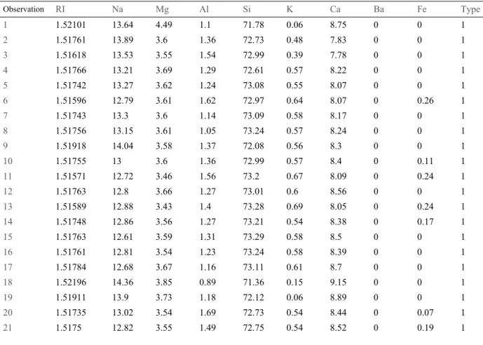
The data ‘Glass’ used in this chapter, taken from UCI Repository Of Machine Learning Databases, containing examples of the chemical analysis of 7 different type of glass. It is a perfect data set for classification and our task is to forecast the type of glass on basis of its chemical analysis.

Observation RI Na Mg Al Si K Ca Ba Fe Type 1 1.52101 13.64 4.49 1.1 71.78 0.06 8.75 0 0 1 2 1.51761 13.89 3.6 1.36 72.73 0.48 7.83 0 0 1 3 1.51618 13.53 3.55 1.54 72.99 0.39 7.78 0 0 1 4 1.51766 13.21 3.69 1.29 72.61 0.57 8.22 0 0 1 5 1.51742 13.27 3.62 1.24 73.08 0.55 8.07 0 0 1 6 1.51596 12.79 3.61 1.62 72.97 0.64 8.07 0 0.26 1 7 1.51743 13.3 3.6 1.14 73.09 0.58 8.17 0 0 1 8 1.51756 13.15 3.61 1.05 73.24 0.57 8.24 0 0 1 9 1.51918 14.04 3.58 1.37 72.08 0.56 8.3 0 0 1 10 1.51755 13 3.6 1.36 72.99 0.57 8.4 0 0.11 1 11 1.51571 12.72 3.46 1.56 73.2 0.67 8.09 0 0.24 1 12 1.51763 12.8 3.66 1.27 73.01 0.6 8.56 0 0 1 13 1.51589 12.88 3.43 1.4 73.28 0.69 8.05 0 0.24 1 14 1.51748 12.86 3.56 1.27 73.21 0.54 8.38 0 0.17 1 15 1.51763 12.61 3.59 1.31 73.29 0.58 8.5 0 0 1 16 1.51761 12.81 3.54 1.23 73.24 0.58 8.39 0 0 1 17 1.51784 12.68 3.67 1.16 73.11 0.61 8.7 0 0 1 18 1.52196 14.36 3.85 0.89 71.36 0.15 9.15 0 0 1 19 1.51911 13.9 3.73 1.18 72.12 0.06 8.89 0 0 1 20 1.51735 13.02 3.54 1.69 72.73 0.54 8.44 0 0.07 1 21 1.5175 12.82 3.55 1.49 72.75 0.54 8.52 0 0.19 1

This dataset containing 214 observation on 10 variables, and the following table provides a basic summary of this dataset.

Table 2. Summary of Data ‘Glass’

Min 1st Qu Median Mean 3rd Qu Max

Ri 1.511 1.517 1.518 1.518 1.519 1.534 Na 10.730 12.910 13.300 13.410 13.820 17.380 Mg 0.000 2.115 3.480 2.685 3.600 4.490 Al 0.290 1.190 1.360 1.445 1.630 3.500 Si 69.810 72.280 72.790 72.650 73.090 75.410 K 0.000 0.123 0.555 0.497 0.610 6.210 Ca 4.430 8.240 8.600 8.957 9.172 16.190 Ba 0.000 0.000 0.000 0.175 0.000 3.150 Fe 0.000 0.000 0.000 0.057 0.100 0.510

Table 3. Quantities for Each Type of Glass

Quantity 70 76 17 13 9 29

We are going to take R package ‘e1071’, which is developed for support vector machine to help us to do the classification and prediction. First of all, we need to start by splitting the data into train and test data set, by randomly select 71 observations (one-third of dataset) as test data and the remains as train data.

In this case, we are going to build our support vector classification nonlinearly, and the kernel we are going to use is radial kernel. Starting with setting cost as 100 and gamma in radial kernel as 1, the support vector classifier will be represented as

𝑓

(

)

𝑝

∑

𝑗= 1

𝑎_𝑖exp

(

|

|

|

|

)

And by taking code ‘svm’ from package ‘e1071’ in R, we got the summary of our model showing below:

Table 4. Summary of Base Model for Data ‘Glass’ Parameters: SVM-Type: C-classification SVM-Kernel: radial cost: 100 gamma: 1 Class 1 2 3 5 6 7 Total

The number of support vector is a measurement of the performance of a certain dataset fits a classification model. The lower the number is, the better it fits in this model.

The next step is to predict the test value, and the way for us to visualize the performance of the accuracy our prediction is to build the confusion matrix, which is also known as ‘the error matrix’.

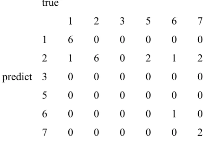
By taking code ‘confusionMatrix’ from package ‘caret’, we obtained the confusion matrix and the summary of this model is showing below:

Confusion Matrix true 1 2 3 5 6 7 1 6 0 0 0 0 0 2 1 6 0 2 1 2 3 0 0 0 0 0 0 5 0 0 0 0 0 0 6 0 0 0 0 1 0 predict 7 0 0 0 0 0 2

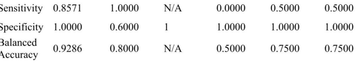
Table 5. Statistics of Base Model for Data ‘Glass’ Overall Statistics:

Accuracy : 0.7143

95% CI : (0.4782, 0.8872) No Information Rate : 0.3333 P-Value [Acc > NIR] : 0.0004045 Statistics by Class:

Sensitivity 0.8571 1.0000 N/A 0.0000 0.5000 0.5000

Specificity 1.0000 0.6000 1 1.0000 1.0000 1.0000

Balanced

Accuracy 0.9286 0.8000 N/A 0.5000 0.7500 0.7500

The accuracy quantifies the performance of a specific support vector machine classification model Balanced accuracy is calculated as the average of the proportion corrects of each class individually. In our case, the overall accuracy is 0.7143. This means if we are going to predict a dataset, the probability of classifying a certain data point to its actual class is 0.7143.

The training accuracy is determined by several factors: cost, type of the kernel, and the parameters in a certain kernel. In our case, for instance, if we change our cost from 100 to 50, the outcomes will become

Table 6. Summary of Adjusted Model 1 for Data ‘Glass’ Parameters: SVM-Type: C-classification SVM-Kernel: radial cost: 50 gamma: 1 Class 1 2 3 5 6 7 Total

It shows from the summary that the number of the support vector is lower than the situation when we set the cost equal to 100. Normally, the number of support vector will decreasing when the cost become lower, since the soft-margin is narrow down.

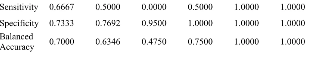
Also, we can get a another confusion matrix from this model. Confusion matrix: true 1 2 3 5 6 7 1 4 4 0 0 0 0 2 1 4 1 1 0 0 3 1 0 0 0 0 0 5 0 0 0 1 0 0 6 0 0 0 0 1 0 predict 7 0 0 0 0 0 3

Table 7. Statistics of Adjusted Model 1 for Data ‘Glass’ Overall Statistics

Accuracy : 0.619

95% CI : (0.3844, 0.8189) No Information Rate : 0.381 P-Value [Acc > NIR] : 0.2313 Statistics by Class:

Sensitivity 0.6667 0.5000 0.0000 0.5000 1.0000 1.0000

Specificity 0.7333 0.7692 0.9500 1.0000 1.0000 1.0000

Balanced

Accuracy 0.7000 0.6346 0.4750 0.7500 1.0000 1.0000

Another factor that can affect the training accuracy is the parameter in the kernel. In our case, gamma is the only parameter which can affect the result. For example, if we change gamma from 1 to 0.5, the outcome will become

Table 8. Summary of Adjusted Model 2 for Data ‘Glass’ Parameters: SVM-Type: C-classification SVM-Kernel: radial cost: 100 gamma: 0.5 Class 1 2 3 5 6 7 Total

Number of support vector 43 49 15 11 8 20 146

Same as the situation when we change the cost from 100 to 50, the number of support vector also decreases when we lower the parameter gamma, since it is also a factor which can affect the range of soft-margin. The summary of confusion matrix shows below: Confusion matrix: true 1 2 3 5 6 7 1 5 3 0 0 0 0 2 0 4 1 1 0 0 predict 3 1 1 0 0 0 0

5 0 0 0 1 0 0

6 0 0 0 0 1 0

7 0 0 0 0 0 3

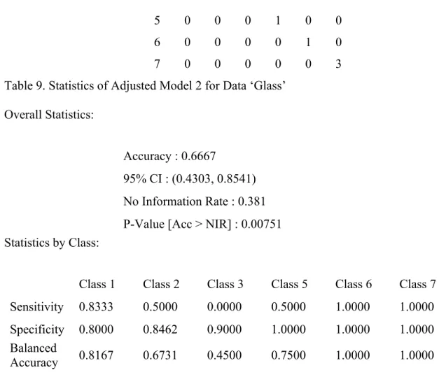
Table 9. Statistics of Adjusted Model 2 for Data ‘Glass’ Overall Statistics:

Accuracy : 0.6667

95% CI : (0.4303, 0.8541) No Information Rate : 0.381 P-Value [Acc > NIR] : 0.00751 Statistics by Class:

Class 1 Class 2 Class 3 Class 5 Class 6 Class 7

Sensitivity 0.8333 0.5000 0.0000 0.5000 1.0000 1.0000

Specificity 0.8000 0.8462 0.9000 1.0000 1.0000 1.0000

Balanced

Accuracy 0.8167 0.6731 0.4500 0.7500 1.0000 1.0000

We can realized in these two cases the training accuracy is lower than the

situation when we set the cost equal to 100 and gamma equal to 1. This is common, even though in both cases, the number of support vector do decrease. This situation is called ‘overfitting’, which occurs when the model is complex, i.e., has too many parameters related to the observation.

Our task is to fit the model to the dataset as accurate as possible, which means we need to find a certain combination of cost and gamma in the kernel. The approach which is commonly used is cross-validation, a model validation technique for assessing how the results of statistical analysis will generalize to an independent data set. It is mainly used in settings where the goal is prediction, and one wants to estimate

how accurately a predictive model will perform in practice. Here we are going to take the approach 10-fold cross-validation, which randomly separate the original dataset in to 10 subset, and on each time select one as a test data and the other nine as training data.

In R, we can write a ‘for loop’ to build this cross-validation. We could set sequence which allows the cost runs from 100 to 1 for 100 times, and set gamma from 0.01 from 1 for 100 times. In each combination, the for loops allows R to test our dataset 10 times where randomly selected 1 subset from the original dataset as the test dataset. This means the R system need to loop 100 × 100 × 10testing subgroup to get the best combination of parameter gamma and constant cost. In this test, the base case is the situation we set gamma equal to 1 and cost equal to 10. The result after this 10-fold cross validation is showing below.

Table 10. Summary of Fittest Model for Data ‘Glass’ Parameters: SVM-Type: C-classification SVM-Kernel: radial cost: 10 gamma: 0.43 Class 1 2 3 5 6 7 Total

Number of support vector 51 53 16 11 7 17 155

The results shows that the highest accuracy occurs when cost equal to 10 and gamma is 0.43. We can realized the number of support vector does not decrease, the reason we mentioned before since the narrower soft margin could cause the overfitting situation.

Confusion matrix: true 1 2 3 5 6 7 1 6 0 0 0 0 0 2 1 6 0 1 1 2 3 0 0 0 0 0 0 5 0 0 0 1 0 0 6 0 0 0 0 1 0 predict 7 0 0 0 0 0 2

Table 11. Statistics of Fittest Model for Data ‘Glass’ Overall Statistics:

Accuracy : 0.7619

95% CI : (0.5283, 0.9178) No Information Rate : 0.3333 P-Value [Acc > NIR] : 7.251e-05

Statistics by Class:

Class 1 Class 2 Class 3 Class 5 Class 6 Class 7

Sensitivity 0.8571 1.0000 N/A 0.5000 0.5000 0.5000

Specificity 1.0000 0.6667 1.0000 1.0000 1.0000 1.0000

Balanced

The highest accuracy calculated by 10-fold cross validation is 0.7619, which is slightly higher than our base case. In fact, in this example, the combination of the original gamma and cost is not the worst situation compare to other cases.

In general, in machine learning cases, we would expect our confusion matrix for prediction has at least 70%-80% accuracy. From this point of view, we cannot conclude that the result of our experiment is inaccurate, however, it is not ideal, technically speaking.

There is two possible reason which cause this situation. The first is the complexity of our observation. The hyperplane could become harder to set along with the increase of the number of parameter. In this example, we have 9 parameters and we can realize that in some situation, even though it shows the accuracy increases in the overall statistics, for a specific class, the balanced accuracy for prediction could possibly decrease.

The second reason is the choice of test dataset. In our experiment, we separated the original dataset into several subset and chose one as a test dataset and loop approach. However, we do not have a ‘unknown’ dataset for prediction, which means this part of dataset is only treated as test dataset, not the training one. The design of our experiment has higher possibility to cause overfitting, which can be an important factor which lower the prediction accuracy.

Chapter 3 SUPPORT VECTOR REGRESSION

This chapter will discuss support vector machine applied to both linear and non-linear regression problem. Our goal is to is to find a function f(x) that has at most ε

as flat as possible. In other words, the data points lie in between the two borders of the margin which is maximized under suitable conditions will avoid outlier inclusion. 3.1 Linear regression

Suppose we are given a set of data

𝐷=

{

(

)

(

)

}

with linear function in form of

𝑓(𝑥) = <𝑤, 𝑥> +𝑏 (3.2) The optimal regression function is given by the minimum of the functional,

𝜙(𝜔, 𝜁) = 1 2∥ 𝜔 ∥ 2_+𝐶 𝑙

∑

where 𝐶> 0 is a pre-specified constant value, determined the trade-off between the flatness of and the amount up to which deviations larger than 𝑓 ε are tolerated, and

are slack variables representing upper and lower constraints on the outputs of the 𝜉‒, 𝜉+

system.

3.1.1 ε-insensitive Loss Function

The ε-insensitive loss function is the following

Figure 3.1 A plot of typical ε-insensitive loss function

This loss function is ideal when small amounts of error are acceptable, which is also refer to a ‘soft-margin’. In ε-insensitive loss function, any points within some selected range ε are considered to have no error at all, which means the ε-insensitive loss function can be represented as

𝐿ℇ(𝑦) =

{

In linear function 𝑓(𝑥) = <𝑤, 𝑥> +𝑏, <𝜔, 𝑥> denotes the dot product in . Since we mentioned before, one of our goal is to ensure the flatness, which means 𝑅𝑑

seeking a small . One of our way is to minimize the norm, i.e. 𝜔 ∥ 𝜔 ∥2= <𝜔, 𝜔>. minimize 1 2∥ 𝜔 ∥ 2 _(3.6) subject to

{

Applying ε-insensitive loss function for minimizing the optimal regression function, minimize (3.8) 1 2∥ 𝜔 ∥ 2 +𝐶∑𝑙_{𝑖= 1}(𝜉‒_𝑖 +𝜉+_𝑖 ) 𝑠𝑢𝑏𝑗𝑒𝑐𝑡 𝑡𝑜

{

Here, the key idea is to construct a Lagrange function (Smola & Scholkopf, 2003). We proceed as follows: 𝐿

(

)

∑

∑

(

)

∑

∑

Here L is the Lagrangian and 𝜂𝑖,𝜂 are Lagrange multipliers. Taking partial

∗ 𝑖,𝛼𝑖,𝛼

∗ 𝑖

derivative of 3.10 with primal variables

(

)

∂_𝑏𝐿= 𝑙

∑

(

)

∑

(

)

Substituting the 3.11-3.13 into L, the solution is given by,

max ‒1 2 𝑙

∑

∑

(

)(

)

∑

(

)

(

) (3.14)

∑

∑

(

)(

)

∑

(

)

∑

(

)

0≤ 𝛼_𝑖,𝛼∗_𝑖 ≤ 𝐶, 𝑖=1,…, 𝑙 (3.16) 𝑙

∑

Equation 3.12 can be rewritten as 𝜔= 𝑙

∑

(

)

∑

(

)

The Karush-Kuhn-Trcker conditions that are satisfied by the solution are,

𝛼_𝑖𝛼∗_𝑖 =0, 𝑖=1,…,𝑙 (3.20)

which is also called complementary slackness (Smola & Scholkopf, 2003). This condition shows that there can never be a set of dual variables 𝛼𝑖,𝛼 which are both

∗ 𝑖

simultaneously nonzero, which allows us to conclude that

𝜀 ‒ 𝑦_𝑖+ <𝜔, 𝑥_𝑖>+𝑏 ≥ 0 𝑎𝑛𝑑 𝜉_𝑖=0 𝑖𝑓 𝛼_𝑖<𝐶 𝜀 ‒ 𝑦_𝑖+ <𝜔, 𝑥_𝑖>+𝑏 ≤ 0 𝑖𝑓 𝛼_𝑖< 0 (3.21)

Therefore, the support vectors are points where exactly one of the Lagrange multipliers is greater than zero. When ε = 0, we get L loss function and the optimization problem simplified, 𝑚𝑖𝑛1 2 𝑙

∑

∑

∑

with constraints, ‒ 𝐶 ≤ 𝛽_𝑖≤ 𝐶, 𝑖=1,…, 𝑙 (3.23) 𝑙

∑

and the regression function is given by Equation 3.2, where 𝜔= 𝑙

∑

(

)

where and are support vectors lie on the edge of the margin.𝑥𝑟 𝑥𝑠

In addition, if 𝜀= 0, the result is just the median regression. 3.1.2 Quadratic Loss Function

The quadratic function is the following

𝐿(𝑓(𝑥)‒ 𝑦) =(𝑓(𝑥)‒ 𝑦)2 (3.26)

Quadratic loss is another function that is well-suited for the purpose of regression problems, although it makes the outliers in the data punished very heavily by the squaring of the error. As a result, datasets must be filtered for outliers first, or else the fit from this loss function may not be desirable.

Same as what we did in 3.1.1, by applying quadratic loss function, the solution is given by, max ‒1 2 𝑙

∑

∑

(

)(

)

∑

(

)

∑

(

(

)

)

The corresponding optimisation can be simplified by exploiting the KKT conditions, which implies 𝛽∗𝑖 =

|

|

𝑚𝑖𝑛1 2 𝑙

∑

∑

∑

∑

∑

and the regression function is given by Equation 3.2, where 𝜔= 𝑙

∑

(

)

3.1.3 Huber Loss Function

Figure 3.3 Huber loss and quadratic loss as a function of 𝑦 ‒ 𝑓(𝑥) 𝐿_{ℎ𝑢𝑏𝑒𝑟}(𝑓(𝑥)‒ 𝑦)

{

Huber proposed the loss function as a robust loss function that has optimal properties when the distribution of the data is unknown (Yeh, Huang & Lee, 2011). Compared to quadratic loss function, Huber loss is less sensitive to outliers in data. As defined above, the Huber loss function is convex in a uniform neighborhood of its minimum 𝑓(𝑥)‒ 𝑦= 0, at the boundary of this uniform neighborhood, the Huber loss function has a differentiable extension to an affine function at points 𝑓(𝑥)‒ 𝑦=‒ 𝜇 and

. These properties allow it to combine much of the sensitivity of the

mean-𝑓(𝑥)‒ 𝑦=𝜇

By applying Huber loss function, the solution is given by, maximize ‒1 2 𝑙

∑

∑

(

)(

)

∑

(

)

∑

(

(

)

)

The resultant optimization problem is, 𝑚𝑖𝑛1 2 𝑙

∑

∑

∑

∑

∑

and the regression function is given by Equation 3.2, where 𝜔= 𝑙

∑

(

)

In the situation of nonlinear support vector regression approach, it is always achieved by mapping into a high dimensional feature space, i.e. there exist a map : 𝑥𝑖 Φ

, which is a space the standard SV linear regression performs. The most widely

𝜒→𝐹 𝐹

adopted method is by using kernel approach.

minimize 1 2∥ 𝜔 ∥ 2 +𝐶∑𝑙_{𝑖= 1}(𝜉‒_𝑖 +𝜉+_𝑖 ) (3.29) 𝑠𝑢𝑏𝑗𝑒𝑐𝑡 𝑡𝑜

{

(

)

where the regression hyperplane is derived as

𝑓(𝑥) = <𝑤, Φ(𝑥) > +𝑏 (3.31)

To solve 3. , one can also introduce the Lagrange function as the linear SVR situation and taking partial derivatives with respect to the primal variables and set the resulting derivatives to zero. The solution is given by

max ‒1 2 𝑙

∑

∑

(

)(

)

∑

∑

∑

Here, 𝐾<𝑥𝑖, 𝑥𝑗> is the kernel function which represents the inner product

.

<Φ(𝑥_𝑖), Φ(𝑥_𝑗) >

The most widely used kernel function is the radial basis function, which is also called Gaussian kernel. The function is defined as

𝐾<𝑥_𝑖, 𝑥_𝑗≥ = <Φ

(

),

(

)

where

|

|

|

|

2

vectors, and γ is the width parameter of Gaussian kernel. Solving 3.33 with the constraints equation, the regression function is given by,

𝑓(𝑥) = 𝑙

∑

(

)

∑

(

)

∑

(

)

As with the SVC the equality constraint may be dropped if the Kernel contains a bias term, b being accommodated within the Kernel function, and the regression function is given by, 𝑓(𝑥) = 𝑙

∑

(

)

2.5 Application of Support Vector Regression to Real World Data

The data ‘Ozone’ used in this chapter, taken from Department of Statistics, UC

Berkeley, containing observation of Los Angeles daily ozone pollution in 1976, and other factors that related to ozone pullution. It is a perfect data set for support vector regression and our task is to predict the daily maximum one-hour-average ozone reading based on the dataset.

Table 12. Los Angeles daily ozone pollution in 1976 (Partial)

2 1 2 5 3 5660 6 NA 38 NA NA -14 NA 300 3 1 3 6 3 5710 4 28 40 NA 2693 -25 47.66 250 4 1 4 7 5 5700 3 37 45 NA 590 -24 55.04 100 5 1 5 1 5 5760 3 51 54 45.32 1450 25 57.02 60 6 1 6 2 6 5720 4 69 35 49.64 1568 15 53.78 60 7 1 7 3 4 5790 6 19 45 46.4 2631 -33 54.14 100 8 1 8 4 4 5790 3 25 55 52.7 554 -28 64.76 250 9 1 9 5 6 5700 3 73 41 48.02 2083 23 52.52 120 10 1 10 6 7 5700 3 59 44 NA 2654 -2 48.38 120 11 1 11 7 4 5770 8 27 54 NA 5000 -19 48.56 120 12 1 12 1 6 5720 3 44 51 54.32 111 9 63.14 150 13 1 13 2 5 5760 6 33 51 57.56 492 -44 64.58 40 14 1 14 3 4 5780 6 19 54 56.12 5000 -44 56.3 200 15 1 15 4 4 5830 3 19 58 62.24 1249 -53 75.74 250 16 1 16 5 7 5870 2 19 61 64.94 5000 -67 65.48 200 17 1 17 6 5 5840 5 19 64 NA 5000 -40 63.32 200 18 1 18 7 9 5780 4 59 67 NA 639 1 66.02 150 19 1 19 1 4 5680 5 73 52 56.48 393 -68 69.8 10 20 1 20 2 3 5720 4 19 54 NA 5000 -66 54.68 140 21 1 21 3 4 5760 3 19 54 53.6 5000 -58 51.98 250 Format: V1. Month V2. Day of month V3. Day of week

V4. Daily maximum one-hour-average ozone reading

V5. 500 millibar pressure height (m) measured at Vandenberg AFB V6. Wind speed (mph) at Los Angeles International Airport (LAX) V7. Humidity (%) at LAX

V8. Temperature (degrees F) measured at Sandburg, CA V9. Temperature (degrees F) measured at El Monte, CA

V10. Inversion base height (feet) at LAX

V11. Pressure gradient (mm Hg) from LAX to Daggett, CA V12. Inversion base temperature (degrees F) at LAX

V13. Visibility (miles) measured at LAX

We are also going to take R package ‘e1071’ as what we did in support vector classification to help us construct regression models and predict. We are going to separate our data into training and testing data, however, since we our task is to build a regression model, we need to omit the missing data in the dataset, which is the observation with parameters show not available in the table.

After omitting the missing data, we separate the observation into 134 observations as training data and 69 observations as testing data, since we are going to construct a one-third test, where we set one-one-third of the dataset as testing data and another part as training data. We are going to construct a nonlinear regression model with ε-insensitive Loss Function. Also, since it is nonlinear regression, we need a kernel to help us construct the model and here we will go with Gaussian kernel. Starting with setting cost as 1000 and gamma in radial kernel as 0.0001 and using code ‘svm’ in package ‘e1071’, we got the summary of our model showing below:

Table 13. Summary of Base Model for Data ‘Ozone’ Parameters:

SVM-Type: eps-regression SVM-Kernel: radial

cost: 1000 gamma: 1e-04

Same as support vector classification, the number of support vector is a

measurement of the performance of a certain dataset fits this regression model. The lower the number is, the better it fits in this model.

The next step is to predict the test value, and the way for us to quantify the performance of fitness of our prediction is to calculate pseudo r square.

𝑅2= 1‒ 𝑙𝑛𝐿(𝑀𝑓𝑢𝑙𝑙)

𝑙𝑛𝐿(𝑀_{𝑖𝑛𝑡𝑒𝑟𝑐𝑒𝑝𝑡}) (3.43)

The equation showing above is called Mcfadden’s pseudo r square, which we are going to use in our prediction, where 𝑙𝑛𝐿(𝑀𝑓𝑢𝑙𝑙) represent log likelihood for model with

predictors, and 𝑙𝑛𝐿(𝑀𝑖𝑛𝑡𝑒𝑟𝑐𝑒𝑝𝑡) represent log likelihood for model withour predictors

(Yeh, Huang & Lee, 2011). The log likelihood of the intercept model is treated as a total sum of squares, and the log likelihood of the full model is treated as the sum of squared errors. The ratio of the likelihoods suggests the level of improvement over the intercept model offered by the full model. A likelihood falls between 0 and 1, and a smaller ratio of log likelihoods indicates that the full model is a far better fit than the intercept model. Thus, if comparing two models on the same data, McFadden’s would be higher for the model with the greater likelihood.

By computing likelihood for both full and intercept models from package ‘e1071’, we obtained the Mcfadden’s pseudo r square equals to be 0.6793. Since the r square is describe to be as large as possible, the next step we are going to do is to change the parameters in our model, which is similar to what we did in Chapter 2. The only 2

parameters which decide r square is cost and gamma in the radial kernel. For example, if we change cost from 1000 to 500, the summary of our model will become

Table 14. Summary of Adjusted Model 1 for Data ‘Ozone’ Parameters:

SVM-Type: eps-regression SVM-Kernel: radial

cost: 500 gamma: 1e-04

Number of Support Vectors: 116

We can see the number of support vectors decrease, which means the new regression model fits our dataset slightly better. Also, by computing the r square, we got the value to be 0.7264, which also confirm our conclusion from summary.

Also, we can change gamma, for example, from 0.0001 to 0.001, and the summary is shown below as

Table 15. Summary of Adjusted Model 2 for Data ‘Ozone’ Parameters:

SVM-Type: eps-regression SVM-Kernel: radial

cost: 1000 gamma: 0.001

Number of Support Vectors: 108

And the r square equals to 0.6789, which is slightly lower than the original model. Since the number of support vector do decrease, we can consider it as an overfitting situation.

Our goal is find a model, which can fit our dataset as accurate as possible, so the approach we are going to take is still cross-validation as we did in Chapter 2. Here, we are going to take a 5-fold cross-validation, where we write a ‘for loop’ to achieve it in R. We could set a sequence which allows the cost runs from 1000 to 100 for 90 times, and set gamma from 0.0001 from 0.01 for 100 times. The base case is showing in our original model where cost is 1000 and gamma is 0.0001.

The result after the cross-validation shows below: Table 16. Summary of Fittest Model for Data ‘Ozone’

Parameters:

SVM-Type: eps-regression SVM-Kernel: radial

cost: 100 gamma: 0.0011

Number of Support Vectors: 102

Here, the r square is equals to 0.7853. From the result, we can realize the number of support vector decreases significantly and meanwhile the r square increase. Since the cost in this model is the lowest model in our sequence and the number of support vector do decrease when we change cost from 1000 to 500, we may assume that the model fits better with the decrease of cost.

In fact, we can plot the r square for this cross-validation with parameter cost and gamma, as seen in Figure 3.4.

Figure 3.4 R square plot for 5-fold cross validation

We can see from this plot that the highest R square appears when cost and gamma are both relatively small. Since we mentioned before the model could be too sensitive for the dataset when we set the cost undersize and the overfitting situation may also appears, we can consider that this regression model with cost 100 and gamma 1 an relatively ideal result.

REFERENCE

James, G., Witten, D., Hastie, T. & Tibshirani, R. (2009). An Introduction to Statistical Learning (2nd ed.). New York: Springer.

Smola, A.J. & Scholkopf, B. (2003). A Tutorial on Support Vector Regression.Statistics and Computing, 14, 199–222.

Yeh, C. Y., Huang, C. W. & Lee, S. J. (2011). A Multiple-kernel support vector regression approach for stock market price forecasting. Expert System with

APPENDICES Appendix A. Glass Data

Observation RI Na Mg Al Si K Ca Ba Fe Type 1 1.52101 13.64 4.49 1.1 71.78 0.06 8.75 0 0 1 2 1.51761 13.89 3.6 1.36 72.73 0.48 7.83 0 0 1 3 1.51618 13.53 3.55 1.54 72.99 0.39 7.78 0 0 1 4 1.51766 13.21 3.69 1.29 72.61 0.57 8.22 0 0 1 5 1.51742 13.27 3.62 1.24 73.08 0.55 8.07 0 0 1

6 1.51596 12.79 3.61 1.62 72.97 0.64 8.07 0 0.26 1 7 1.51743 13.3 3.6 1.14 73.09 0.58 8.17 0 0 1 8 1.51756 13.15 3.61 1.05 73.24 0.57 8.24 0 0 1 9 1.51918 14.04 3.58 1.37 72.08 0.56 8.3 0 0 1 10 1.51755 13 3.6 1.36 72.99 0.57 8.4 0 0.11 1 11 1.51571 12.72 3.46 1.56 73.2 0.67 8.09 0 0.24 1 12 1.51763 12.8 3.66 1.27 73.01 0.6 8.56 0 0 1 13 1.51589 12.88 3.43 1.4 73.28 0.69 8.05 0 0.24 1 14 1.51748 12.86 3.56 1.27 73.21 0.54 8.38 0 0.17 1 15 1.51763 12.61 3.59 1.31 73.29 0.58 8.5 0 0 1 16 1.51761 12.81 3.54 1.23 73.24 0.58 8.39 0 0 1 17 1.51784 12.68 3.67 1.16 73.11 0.61 8.7 0 0 1 18 1.52196 14.36 3.85 0.89 71.36 0.15 9.15 0 0 1 19 1.51911 13.9 3.73 1.18 72.12 0.06 8.89 0 0 1 20 1.51735 13.02 3.54 1.69 72.73 0.54 8.44 0 0.07 1 21 1.5175 12.82 3.55 1.49 72.75 0.54 8.52 0 0.19 1 22 1.51966 14.77 3.75 0.29 72.02 0.03 9 0 0 1 23 1.51736 12.78 3.62 1.29 72.79 0.59 8.7 0 0 1 24 1.51751 12.81 3.57 1.35 73.02 0.62 8.59 0 0 1 25 1.5172 13.38 3.5 1.15 72.85 0.5 8.43 0 0 1 26 1.51764 12.98 3.54 1.21 73 0.65 8.53 0 0 1 27 1.51793 13.21 3.48 1.41 72.64 0.59 8.43 0 0 1 28 1.51721 12.87 3.48 1.33 73.04 0.56 8.43 0 0 1 29 1.51768 12.56 3.52 1.43 73.15 0.57 8.54 0 0 1 30 1.51784 13.08 3.49 1.28 72.86 0.6 8.49 0 0 1 31 1.51768 12.65 3.56 1.3 73.08 0.61 8.69 0 0.14 1 32 1.51747 12.84 3.5 1.14 73.27 0.56 8.55 0 0 1 33 1.51775 12.85 3.48 1.23 72.97 0.61 8.56 0.09 0.22 1 34 1.51753 12.57 3.47 1.38 73.39 0.6 8.55 0 0.06 1 35 1.51783 12.69 3.54 1.34 72.95 0.57 8.75 0 0 1 36 1.51567 13.29 3.45 1.21 72.74 0.56 8.57 0 0 1 Observation RI Na Mg Al Si K Ca Ba Fe Type 37 1.51909 13.89 3.53 1.32 71.81 0.51 8.78 0.11 0 1 38 1.51797 12.74 3.48 1.35 72.96 0.64 8.68 0 0 1 39 1.52213 14.21 3.82 0.47 71.77 0.11 9.57 0 0 1 40 1.52213 14.21 3.82 0.47 71.77 0.11 9.57 0 0 1 41 1.51793 12.79 3.5 1.12 73.03 0.64 8.77 0 0 1 42 1.51755 12.71 3.42 1.2 73.2 0.59 8.64 0 0 1 43 1.51779 13.21 3.39 1.33 72.76 0.59 8.59 0 0 1 44 1.5221 13.73 3.84 0.72 71.76 0.17 9.74 0 0 1

46 1.519 13.49 3.48 1.35 71.95 0.55 9 0 0 1 47 1.51869 13.19 3.37 1.18 72.72 0.57 8.83 0 0.16 1 48 1.52667 13.99 3.7 0.71 71.57 0.02 9.82 0 0.1 1 49 1.52223 13.21 3.77 0.79 71.99 0.13 10.02 0 0 1 50 1.51898 13.58 3.35 1.23 72.08 0.59 8.91 0 0 1 51 1.5232 13.72 3.72 0.51 71.75 0.09 10.06 0 0.16 1 52 1.51926 13.2 3.33 1.28 72.36 0.6 9.14 0 0.11 1 53 1.51808 13.43 2.87 1.19 72.84 0.55 9.03 0 0 1 54 1.51837 13.14 2.84 1.28 72.85 0.55 9.07 0 0 1 55 1.51778 13.21 2.81 1.29 72.98 0.51 9.02 0 0.09 1 56 1.51769 12.45 2.71 1.29 73.7 0.56 9.06 0 0.24 1 57 1.51215 12.99 3.47 1.12 72.98 0.62 8.35 0 0.31 1 58 1.51824 12.87 3.48 1.29 72.95 0.6 8.43 0 0 1 59 1.51754 13.48 3.74 1.17 72.99 0.59 8.03 0 0 1 60 1.51754 13.39 3.66 1.19 72.79 0.57 8.27 0 0.11 1 61 1.51905 13.6 3.62 1.11 72.64 0.14 8.76 0 0 1 62 1.51977 13.81 3.58 1.32 71.72 0.12 8.67 0.69 0 1 63 1.52172 13.51 3.86 0.88 71.79 0.23 9.54 0 0.11 1 64 1.52227 14.17 3.81 0.78 71.35 0 9.69 0 0 1 65 1.52172 13.48 3.74 0.9 72.01 0.18 9.61 0 0.07 1 66 1.52099 13.69 3.59 1.12 71.96 0.09 9.4 0 0 1 67 1.52152 13.05 3.65 0.87 72.22 0.19 9.85 0 0.17 1 68 1.52152 13.05 3.65 0.87 72.32 0.19 9.85 0 0.17 1 69 1.52152 13.12 3.58 0.9 72.2 0.23 9.82 0 0.16 1 70 1.523 13.31 3.58 0.82 71.99 0.12 10.17 0 0.03 1 71 1.51574 14.86 3.67 1.74 71.87 0.16 7.36 0 0.12 2 72 1.51848 13.64 3.87 1.27 71.96 0.54 8.32 0 0.32 2 73 1.51593 13.09 3.59 1.52 73.1 0.67 7.83 0 0 2 74 1.51631 13.34 3.57 1.57 72.87 0.61 7.89 0 0 2 75 1.51596 13.02 3.56 1.54 73.11 0.72 7.9 0 0 2 76 1.5159 13.02 3.58 1.51 73.12 0.69 7.96 0 0 2 Observation RI Na Mg Al Si K Ca Ba Fe Type 77 1.51645 13.44 3.61 1.54 72.39 0.66 8.03 0 0 2 78 1.51627 13 3.58 1.54 72.83 0.61 8.04 0 0 2 79 1.51613 13.92 3.52 1.25 72.88 0.37 7.94 0 0.14 2 80 1.5159 12.82 3.52 1.9 72.86 0.69 7.97 0 0 2 81 1.51592 12.86 3.52 2.12 72.66 0.69 7.97 0 0 2 82 1.51593 13.25 3.45 1.43 73.17 0.61 7.86 0 0 2 83 1.51646 13.41 3.55 1.25 72.81 0.68 8.1 0 0 2 84 1.51594 13.09 3.52 1.55 72.87 0.68 8.05 0 0.09 2 85 1.51409 14.25 3.09 2.08 72.28 1.1 7.08 0 0 2

86 1.51625 13.36 3.58 1.49 72.72 0.45 8.21 0 0 2 87 1.51569 13.24 3.49 1.47 73.25 0.38 8.03 0 0 2 88 1.51645 13.4 3.49 1.52 72.65 0.67 8.08 0 0.1 2 89 1.51618 13.01 3.5 1.48 72.89 0.6 8.12 0 0 2 90 1.5164 12.55 3.48 1.87 73.23 0.63 8.08 0 0.09 2 91 1.51841 12.93 3.74 1.11 72.28 0.64 8.96 0 0.22 2 92 1.51605 12.9 3.44 1.45 73.06 0.44 8.27 0 0 2 93 1.51588 13.12 3.41 1.58 73.26 0.07 8.39 0 0.19 2 94 1.5159 13.24 3.34 1.47 73.1 0.39 8.22 0 0 2 95 1.51629 12.71 3.33 1.49 73.28 0.67 8.24 0 0 2 96 1.5186 13.36 3.43 1.43 72.26 0.51 8.6 0 0 2 97 1.51841 13.02 3.62 1.06 72.34 0.64 9.13 0 0.15 2 98 1.51743 12.2 3.25 1.16 73.55 0.62 8.9 0 0.24 2 99 1.51689 12.67 2.88 1.71 73.21 0.73 8.54 0 0 2 100 1.51811 12.96 2.96 1.43 72.92 0.6 8.79 0.14 0 2 101 1.51655 12.75 2.85 1.44 73.27 0.57 8.79 0.11 0.22 2 102 1.5173 12.35 2.72 1.63 72.87 0.7 9.23 0 0 2 103 1.5182 12.62 2.76 0.83 73.81 0.35 9.42 0 0.2 2 104 1.52725 13.8 3.15 0.66 70.57 0.08 11.64 0 0 2 105 1.5241 13.83 2.9 1.17 71.15 0.08 10.79 0 0 2 106 1.52475 11.45 0 1.88 72.19 0.81 13.24 0 0.34 2 107 1.53125 10.73 0 2.1 69.81 0.58 13.3 3.15 0.28 2 108 1.53393 12.3 0 1 70.16 0.12 16.19 0 0.24 2 109 1.52222 14.43 0 1 72.67 0.1 11.52 0 0.08 2 110 1.51818 13.72 0 0.56 74.45 0 10.99 0 0 2 111 1.52664 11.23 0 0.77 73.21 0 14.68 0 0 2 112 1.52739 11.02 0 0.75 73.08 0 14.96 0 0 2 113 1.52777 12.64 0 0.67 72.02 0.06 14.4 0 0 2 114 1.51892 13.46 3.83 1.26 72.55 0.57 8.21 0 0.14 2 115 1.51847 13.1 3.97 1.19 72.44 0.6 8.43 0 0 2 116 1.51846 13.41 3.89 1.33 72.38 0.51 8.28 0 0 2 Observation RI Na Mg Al Si K Ca Ba Fe Type 117 1.51829 13.24 3.9 1.41 72.33 0.55 8.31 0 0.1 2 118 1.51708 13.72 3.68 1.81 72.06 0.64 7.88 0 0 2 119 1.51673 13.3 3.64 1.53 72.53 0.65 8.03 0 0.29 2 120 1.51652 13.56 3.57 1.47 72.45 0.64 7.96 0 0 2 121 1.51844 13.25 3.76 1.32 72.4 0.58 8.42 0 0 2 122 1.51663 12.93 3.54 1.62 72.96 0.64 8.03 0 0.21 2 123 1.51687 13.23 3.54 1.48 72.84 0.56 8.1 0 0 2 124 1.51707 13.48 3.48 1.71 72.52 0.62 7.99 0 0 2

126 1.51872 12.93 3.66 1.56 72.51 0.58 8.55 0 0.12 2 127 1.51667 12.94 3.61 1.26 72.75 0.56 8.6 0 0 2 128 1.52081 13.78 2.28 1.43 71.99 0.49 9.85 0 0.17 2 129 1.52068 13.55 2.09 1.67 72.18 0.53 9.57 0.27 0.17 2 130 1.5202 13.98 1.35 1.63 71.76 0.39 10.56 0 0.18 2 131 1.52177 13.75 1.01 1.36 72.19 0.33 11.14 0 0 2 132 1.52614 13.7 0 1.36 71.24 0.19 13.44 0 0.1 2 133 1.51813 13.43 3.98 1.18 72.49 0.58 8.15 0 0 2 134 1.518 13.71 3.93 1.54 71.81 0.54 8.21 0 0.15 2 135 1.51811 13.33 3.85 1.25 72.78 0.52 8.12 0 0 2 136 1.51789 13.19 3.9 1.3 72.33 0.55 8.44 0 0.28 2 137 1.51806 13 3.8 1.08 73.07 0.56 8.38 0 0.12 2 138 1.51711 12.89 3.62 1.57 72.96 0.61 8.11 0 0 2 139 1.51674 12.79 3.52 1.54 73.36 0.66 7.9 0 0 2 140 1.51674 12.87 3.56 1.64 73.14 0.65 7.99 0 0 2 141 1.5169 13.33 3.54 1.61 72.54 0.68 8.11 0 0 2 142 1.51851 13.2 3.63 1.07 72.83 0.57 8.41 0.09 0.17 2 143 1.51662 12.85 3.51 1.44 73.01 0.68 8.23 0.06 0.25 2 144 1.51709 13 3.47 1.79 72.72 0.66 8.18 0 0 2 145 1.5166 12.99 3.18 1.23 72.97 0.58 8.81 0 0.24 2 146 1.51839 12.85 3.67 1.24 72.57 0.62 8.68 0 0.35 2 147 1.51769 13.65 3.66 1.11 72.77 0.11 8.6 0 0 3 148 1.5161 13.33 3.53 1.34 72.67 0.56 8.33 0 0 3 149 1.5167 13.24 3.57 1.38 72.7 0.56 8.44 0 0.1 3 150 1.51643 12.16 3.52 1.35 72.89 0.57 8.53 0 0 3 151 1.51665 13.14 3.45 1.76 72.48 0.6 8.38 0 0.17 3 152 1.52127 14.32 3.9 0.83 71.5 0 9.49 0 0 3 153 1.51779 13.64 3.65 0.65 73 0.06 8.93 0 0 3 154 1.5161 13.42 3.4 1.22 72.69 0.59 8.32 0 0 3 155 1.51694 12.86 3.58 1.31 72.61 0.61 8.79 0 0 3 156 1.51646 13.04 3.4 1.26 73.01 0.52 8.58 0 0 3 Observation RI Na Mg Al Si K Ca Ba Fe Type 157 1.51655 13.41 3.39 1.28 72.64 0.52 8.65 0 0 3 158 1.52121 14.03 3.76 0.58 71.79 0.11 9.65 0 0 3 159 1.51776 13.53 3.41 1.52 72.04 0.58 8.79 0 0 3 160 1.51796 13.5 3.36 1.63 71.94 0.57 8.81 0 0.09 3 161 1.51832 13.33 3.34 1.54 72.14 0.56 8.99 0 0 3 162 1.51934 13.64 3.54 0.75 72.65 0.16 8.89 0.15 0.24 3 163 1.52211 14.19 3.78 0.91 71.36 0.23 9.14 0 0.37 3 164 1.51514 14.01 2.68 3.5 69.89 1.68 5.87 2.2 0 5 165 1.51915 12.73 1.85 1.86 72.69 0.6 10.09 0 0 5

166 1.52171 11.56 1.88 1.56 72.86 0.47 11.41 0 0 5 167 1.52151 11.03 1.71 1.56 73.44 0.58 11.62 0 0 5 168 1.51969 12.64 0 1.65 73.75 0.38 11.53 0 0 5 169 1.51666 12.86 0 1.83 73.88 0.97 10.17 0 0 5 170 1.51994 13.27 0 1.76 73.03 0.47 11.32 0 0 5 171 1.52369 13.44 0 1.58 72.22 0.32 12.24 0 0 5 172 1.51316 13.02 0 3.04 70.48 6.21 6.96 0 0 5 173 1.51321 13 0 3.02 70.7 6.21 6.93 0 0 5 174 1.52043 13.38 0 1.4 72.25 0.33 12.5 0 0 5 175 1.52058 12.85 1.61 2.17 72.18 0.76 9.7 0.24 0.51 5 176 1.52119 12.97 0.33 1.51 73.39 0.13 11.27 0 0.28 5 177 1.51905 14 2.39 1.56 72.37 0 9.57 0 0 6 178 1.51937 13.79 2.41 1.19 72.76 0 9.77 0 0 6 179 1.51829 14.46 2.24 1.62 72.38 0 9.26 0 0 6 180 1.51852 14.09 2.19 1.66 72.67 0 9.32 0 0 6 181 1.51299 14.4 1.74 1.54 74.55 0 7.59 0 0 6 182 1.51888 14.99 0.78 1.74 72.5 0 9.95 0 0 6 183 1.51916 14.15 0 2.09 72.74 0 10.88 0 0 6 184 1.51969 14.56 0 0.56 73.48 0 11.22 0 0 6 185 1.51115 17.38 0 0.34 75.41 0 6.65 0 0 6 186 1.51131 13.69 3.2 1.81 72.81 1.76 5.43 1.19 0 7 187 1.51838 14.32 3.26 2.22 71.25 1.46 5.79 1.63 0 7 188 1.52315 13.44 3.34 1.23 72.38 0.6 8.83 0 0 7 189 1.52247 14.86 2.2 2.06 70.26 0.76 9.76 0 0 7 190 1.52365 15.79 1.83 1.31 70.43 0.31 8.61 1.68 0 7 191 1.51613 13.88 1.78 1.79 73.1 0 8.67 0.76 0 7 192 1.51602 14.85 0 2.38 73.28 0 8.76 0.64 0.09 7 193 1.51623 14.2 0 2.79 73.46 0.04 9.04 0.4 0.09 7 194 1.51719 14.75 0 2 73.02 0 8.53 1.59 0.08 7 195 1.51683 14.56 0 1.98 73.29 0 8.52 1.57 0.07 7 196 1.51545 14.14 0 2.68 73.39 0.08 9.07 0.61 0.05 7 Observation RI Na Mg Al Si K Ca Ba Fe Type 197 1.51556 13.87 0 2.54 73.23 0.14 9.41 0.81 0.01 7 198 1.51727 14.7 0 2.34 73.28 0 8.95 0.66 0 7 199 1.51531 14.38 0 2.66 73.1 0.04 9.08 0.64 0 7 200 1.51609 15.01 0 2.51 73.05 0.05 8.83 0.53 0 7 201 1.51508 15.15 0 2.25 73.5 0 8.34 0.63 0 7 202 1.51653 11.95 0 1.19 75.18 2.7 8.93 0 0 7 203 1.51514 14.85 0 2.42 73.72 0 8.39 0.56 0 7 204 1.51658 14.8 0 1.99 73.11 0 8.28 1.71 0 7

206 1.51732 14.95 0 1.8 72.99 0 8.61 1.55 0 7 207 1.51645 14.94 0 1.87 73.11 0 8.67 1.38 0 7 208 1.51831 14.39 0 1.82 72.86 1.41 6.47 2.88 0 7 209 1.5164 14.37 0 2.74 72.85 0 9.45 0.54 0 7 210 1.51623 14.14 0 2.88 72.61 0.08 9.18 1.06 0 7 211 1.51685 14.92 0 1.99 73.06 0 8.4 1.59 0 7 212 1.52065 14.36 0 2.02 73.42 0 8.44 1.64 0 7 213 1.51651 14.38 0 1.94 73.61 0 8.48 1.57 0 7 214 1.51711 14.23 0 2.08 73.36 0 8.62 1.67 0 7

Appendix B. Ozone Data

Observation V1 V2 V3 V4 V5 V6 V7 V8 V9 V10 V11 V12 V13 16 1 16 5 7 5870 2 19 61 64.94 5000 -67 65.48 200 17 1 17 6 5 5840 5 19 64 NA 5000 -40 63.32 200 18 1 18 7 9 5780 4 59 67 NA 639 1 66.02 150 19 1 19 1 4 5680 5 73 52 56.48 393 -68 69.8 10 20 1 20 2 3 5720 4 19 54 NA 5000 -66 54.68 140

21 1 21 3 4 5760 3 19 54 53.6 5000 -58 51.98 250 22 1 22 4 4 5730 4 26 58 52.7 5000 -26 51.98 200 23 1 23 5 5 5700 5 59 69 51.08 3044 18 52.88 150 24 1 24 6 6 5650 5 70 51 NA 3641 23 47.66 140 25 1 25 7 9 5680 3 64 53 NA 111 -10 59.54 50 26 1 26 1 5 5780 3 NA 56 53.6 692 -25 67.1 0 27 1 27 2 6 5820 5 19 59 59.36 597 -52 70.52 70 28 1 28 3 6 5830 4 NA 59 60.08 NA -44 NA 150 29 1 29 4 6 5810 5 19 64 56.66 1791 -15 64.76 150 30 1 30 5 11 5790 3 28 63 57.38 793 -15 65.84 120 31 1 31 6 10 5800 2 32 63 NA 531 -38 75.92 40 32 2 1 7 7 5820 5 19 62 NA 419 -29 75.74 120 33 2 2 1 12 5770 8 76 63 57.2 816 -7 66.2 6 34 2 3 2 9 5670 3 69 54 45.5 3651 62 49.1 30 35 2 4 3 2 5590 3 76 36 37.4 5000 70 37.94 100 36 2 5 4 3 5410 6 64 31 32.18 5000 28 32.36 200 37 2 6 5 3 5350 7 62 30 32.54 1341 18 45.86 60 38 2 7 6 2 5480 9 72 36 NA 5000 0 38.66 350 39 2 8 7 3 5600 7 76 42 NA 3799 -18 45.86 250 40 2 9 1 3 5490 11 72 37 38.48 5000 32 38.12 350 41 2 10 2 4 5560 10 72 41 40.46 5000 -1 37.58 300 42 2 11 3 6 5700 3 32 46 NA 5000 -30 45.86 300 43 2 12 4 8 5680 5 50 51 47.12 5000 -8 45.5 300 44 2 13 5 6 5700 4 86 55 49.28 2398 21 53.78 200 45 2 14 6 4 5650 5 61 41 NA 5000 51 36.32 100 46 2 15 7 3 5610 5 62 41 NA 4281 42 41.36 250 47 2 16 1 7 5730 5 66 49 NA 1161 27 52.88 200 48 2 17 2 11 5770 5 68 45 52.88 2778 2 55.76 200 Observation V1 V2 V3 V4 V5 V6 V7 V8 V9 V10 V11 V12 V13 49 2 18 3 13 5770 3 82 55 55.4 442 26 58.28 40 50 2 19 4 4 5700 5 NA 45 38.12 NA 82 NA 2 51 2 20 5 6 5690 8 21 41 43.88 5000 -30 42.26 300 52 2 21 6 5 5700 3 19 45 NA 5000 -53 43.88 300 53 2 22 7 4 5730 11 19 51 NA 5000 -43 49.1 300 54 2 23 1 4 5690 7 19 53 50.18 5000 7 49.1 300

55 2 24 2 6 5640 5 68 50 37.4 5000 24 42.08 300 56 2 25 3 10 5720 6 63 60 53.06 1341 19 59.18 150 57 2 26 4 15 5740 3 54 54 56.48 1318 2 64.58 150 58 2 27 5 23 5740 3 47 53 58.82 885 -4 67.1 80 59 2 28 6 17 5740 3 56 53 NA 360 3 67.1 40 60 2 29 7 7 5670 7 61 44 NA 3497 73 49.46 40 61 3 1 1 2 5550 10 74 40 38.84 5000 73 40.1 80 62 3 2 2 3 5470 7 46 30 29.66 5000 44 29.3 300 63 3 3 3 3 5320 11 45 25 27.68 5000 39 27.5 200 64 3 4 4 5 NA 8 33 39 30.2 5000 15 30.02 500 65 3 5 5 4 5530 3 43 40 36.14 5000 -12 33.62 140 66 3 6 6 6 5600 3 21 45 NA 5000 -2 39.02 140 67 3 7 7 7 5660 7 57 51 NA 5000 30 42.08 140 68 3 8 1 7 5580 5 42 48 40.64 3608 24 39.38 100 69 3 9 2 6 5510 5 50 45 36.86 5000 38 32.9 140 70 3 10 3 3 5530 5 61 47 33.8 5000 56 35.6 200 71 3 11 4 2 5620 9 61 43 37.04 5000 66 34.34 120 72 3 12 5 8 5690 0 60 49 46.04 613 -27 59.72 300 73 3 13 6 12 5760 4 31 56 NA 334 -9 64.4 300 74 3 14 7 12 5740 3 66 53 NA 567 13 61.88 150 75 3 15 1 16 5780 5 53 61 57.92 488 -20 64.94 2 76 3 16 2 9 5790 2 42 63 57.02 531 -15 71.06 50 77 3 17 3 24 5760 3 60 70 58.64 508 7 66.56 70 78 3 18 4 13 5700 4 82 57 50.36 1571 68 56.3 17 79 3 19 5 8 5680 4 57 35 40.1 721 28 55.4 140 80 3 20 6 10 5720 5 21 52 NA 505 -49 67.28 140 81 3 21 7 8 5720 5 19 59 NA 377 -27 73.22 300 82 3 22 1 9 5730 4 32 67 59.54 442 -9 75.74 200 Observation V1 V2 V3 V4 V5 V6 V7 V8 V9 V10 V11 V12 V13 83 3 23 2 10 5710 5 77 57 57.38 902 54 60.44 250 84 3 24 3 13 5750 6 70 NA 56.3 3188 53 58.64 80 85 3 25 4 14 5720 4 71 42 44.96 1381 4 56.3 60 86 3 26 5 9 5710 3 19 55 51.8 5000 -16 50 100 87 3 27 6 11 5600 6 45 40 NA 5000 38 46.94 150 88 3 28 7 7 5630 4 44 39 NA 1302 40 52.7 150

89 3 29 1 9 5690 7 70 57 46.58 1292 -5 53.6 200 90 3 30 2 12 5730 6 45 58 52.52 5000 -14 52.7 100 91 3 31 3 12 5710 3 46 62 52.52 472 34 62.96 300 92 4 1 4 8 5610 6 50 51 50 1404 42 54.5 120 93 4 2 5 9 5680 5 69 61 51.44 944 35 55.76 100 94 4 3 6 5 5620 6 67 34 NA 5000 75 35.24 200 95 4 4 7 4 5420 7 69 35 NA 5000 41 30.92 200 96 4 5 1 4 5540 5 54 35 33.26 5000 62 33.44 200 97 4 6 2 9 5590 6 51 48 38.12 5000 44 42.08 300 98 4 7 3 13 5690 6 63 59 52.88 2014 31 53.42 300 99 4 8 4 5 5550 7 63 41 37.5