On the algebraic construction
of sparse multilevel approximations
of elliptic tensor product problems
H. Harbrecht and P. Zaspel
Departement Mathematik und Informatik Preprint No. 2018-01
Fachbereich Mathematik January 2018
Universit¨at Basel
On the algebraic construction of sparse multilevel
approximations of elliptic tensor product problems
H. Harbrecht∗ P. Zaspel∗ January 31, 2018
Abstract
We consider the solution of elliptic problems on the tensor product of two physical domains as e.g. present in the approximation of the so-lution covariance of elliptic partial differential equations with random input. Previous sparse approximation approaches used a geometrically constructed multilevel hierarchy. Instead, we construct this hierarchy for a given discretized problem by means of the algebraic multigrid method (AMG). Thereby, we are able to apply the sparse grid com-bination technique to problems given on complex geometries and for discretizations arising from unstructured grids, which was not feasible before. Numerical results show that our algebraic construction exhibits the same convergence behaviour as the geometric construction, while being applicable even in black-box type PDE solvers.
1
Introduction
The solution of elliptic problems on tensor products of a polygonally bounded domain Ω⊂Rd with e.g.d= 2,3 given by
(∆⊗∆)u=f on Ω×Ω, u= 0 on ∂(Ω×Ω),
is an important high-dimensional problem. As an example, this problem shows up in the estimation of the output covariance of an elliptic partial differential equation with random input data that is given on a domain Ω, see [11, 13, 18, 19] for example. The problem becomes high-dimensional since the dimensionality of the elliptic problem on Ω is doubled. In case of real-world problems ind= 3, we end up solving a six-dimensional problem, which might become prohibitively expensive.
Recently, there have been developments to overcome this strong limita-tion. These developments are based on the introduction of a geometrically
constructed multilevel frame, i.e. a hierarchy of discretizations of the elliptic problem on Ω. The multilevel frame gives rise to a sparse approximation with respect to the interaction of the involved domains in Ω×Ω [14, 18, 19]. It has been shown that the sparse approximation allows to solve the ten-sor product problem at a computational complexity that stays essentially (i.e. up to a poly-logarithmic factor) proportional to the number of degrees of freedom to discretize the domain Ω. In a more recent work by one of the au-thors [13], it has been shown that the sparse approximation can equivalently be replaced by the sparse grid combination technique [4, 8, 10, 15]. This further reduces the computational work and facilitates the implementation. However, the currently available geometric construction of the multilevel hierarchy imposes limitations on the discretization in context of real-world problems. First, the coarsest mesh in the hierarchy of discretizations has to fully represent the boundary of the geometry Ω. This either limits the types of geometry to consider or the computational efficiency (in case even the coarsest mesh has to be fine at the boundary). Second, the use of a fully unstructured mesh becomes barely possible, since we are missing a coarsening strategy for such a mesh.
This work introduces algebraically constructed multilevel hierarchies [7, 9, 23] for the solution of elliptic problems on tensor product domains. While previous works [13, 14] first constructed the multilevel hierarchy of meshes and then discretized the problem by finite elements, the new approach first discretizes the problem on Ω on the finest (potentially unstructured) mesh and then constructs coarser versions of the linear system resulting from the fine discretization. The coarser problems are generated using algebraic coarsening known from the classicalRuge-St¨uben algebraic multigrid (AMG) [17, 20]. The algebraic construction of multilevel hieararchies for frames has been previously discussed in context of optimal complexity solvers for elliptic problems in [23]. However, it has not been applied in the context of sparse approximation yet. Note that, by construction, our new approach allows us to overcome both the limitations in presence of complex geometries and the requirements on the structure of the mesh. Moreover, it perfectly fits into the context of black-box type PDE solvers.
As it is well-known, a full theory for algebraic multigrid methods, espe-cially in the multilevel context and on unstructured grids, is still to be de-veloped. Nevertheless, this technique is extremely popular as solver in real-world applications and, usually, empirically shows the same performance as geometric multigrid. This work follows the same spirit and focuses on the formal construction and the empirical analysis of the resulting numerical method. Thereby, we are able to match the convergence results available for geometrically constructed sparse approximations, while being able to apply this approach to complex geometries and unstructured grids in a black-box fashion.
con-struction is introduced to the tensor product problem with sparse approx-imation and the sparse grid combination technique in Section 3. Section 4 briefly discusses the implementation. In Section 5, we give a series of numer-ical examples with empirnumer-ical error analysis. Finally, Section 6 summarizes this work.
2
Algebraic multilevel constructions
In our algebraic construction, we aim at replacing classical multilevel dis-cretizations for elliptic partial differential equations by a purely matrix-based construction. That is, we consider an elliptic partial differential equation
−∆u=f on Ω
u= 0 on ∂Ω (1)
on a polygonally bounded domain Ω ⊂ Rd. This problem has been dis-cretized by some method on a discretization levelJ, leading to a system of linear equations
AJuJ =fJ, (2) where AJ ∈ RNJ×NJ is an M-matrix and uJ,fJ ∈ RNj. In case of the discretization by finite elements,AJ corresponds to the stiffness matrix and
fJ is the load vector, obtained by, for example, using the mass matrix
MJ and interpolation. Moreover, we identify each variable uJ,i in uJ = (uJ,1. . . uJ,NJ)> by its index i and introduce the corresponding index set
DJ :={1, . . . , NJ} for discretization levelJ.
2.1 Multilevel hierarchy of discretized problems
The objective is to construct from (2) a hierarchy of systems of linear equa-tions
Ajuj =fj, j= 0, . . . , J , (3) which are similar to discretizations on different geometric refinement levels. Especially, we intend to do this in a purely matrix-based, i.e. algebraic, way by using coarsening and transfer operators from algebraic multigrid (AMG) [20]. To this end, we first introduce a construction method for a hierarchy of variable sets
D0⊂ D1 ⊂. . .⊂ DJ (4) of sizes
Algorithm 1 Standard coarsening algorithm [21] Require: levelj 1: functionAMGstandardCoarsening 2: Fj :=∅,Dj−1 :=∅, Uj :=Dj 3: fori∈Uj do 4: λj(i) := Sj(i)>∩Uj + 2Sj(i)>∩Fj 5: while ∃is.th.λj(i)6= 0 do
6: findimax:= arg maxiλj(i)
7: Dj−1 :=Dj−1∪ {imax} 8: Uj :=Uj\ {imax} 9: forj∈(Sj(i)>∩Uj) do 10: Fj :=Fj∪ {j} 11: Uj :=Uj \ {j} 12: fori∈Uj do 13: λj(i) := Sj(i)>∩Uj + 2Sj(i)>∩Fj 14: return Dj−1, Fj
In classical Ruge-St¨uben AMG [17, 21], this is achieved by recursively splitting the set of variables Dj on levelj into a set of coarse and fine grid variables
Dj =Dj−1 ·∪ Fj.
Each fine grid variable is supposed to be in the neighborhood of an appro-priate amount of strongly coupled coarse grid variables, where we define the neighborhood of a variable i∈ Dj by
Nj(i) :={i0 ∈ Dj :i0 6=i, aj,ii0 6= 0},
whereAj = (aj,ii0)Ni,ij0=1. That is, we consider neighborhoods between vari-ables by reinterpreting the system matrix Aj as the adjacency matrix of a graph with edges between nodes for each non-zero matrix entry. Moreover, the set of neighboring strongly negatively coupled variables of a variableiis
Sj(i) :=
n
i0 ∈ Nj(i)| −aj,ii0 ≥strmax k |aj,ik|
o
with a strength measure 0< str <1. The standard coarsening procedure, cf. Algorithm 1 [21], builds an appropriate splitting Dj =Dj−1 ·∪ Fj based on these considerations. It also involves the setsSj(i)>, which are given by
Sj(i)>:={i0 ∈ Dj :i∈ Sj(i0)}.
In order to define the hierarchy of linear systems (3), we further need a means to transfer information between two consecutive levels j and j+ 1.
This is done by prolongation operators Pjj+1 ∈ RNj+1×Nj and restriction
operators Pjj+1 ∈ RNj×Nj+1. Prolongation and restriction are done in a purely algebraic way based on AMG. Instandard interpolation [21], which is one possible type of algebraic prolongation, data given on a fine grid node i∈ Fj are interpolated from the set of interpolatory variables
Ij(i) := (Dj−1∩ Sj(i))∩ [ i0∈Fj∩Sj(i) Dj−1∩ Sj(i0) .
Thus, it is interpolated from strongly negatively coupled coarse grid points and all coarse grid points that are strongly negatively coupled to strongly negatively coupled fine grid points. The exact choice of prolongation / interpolation weights is known from literature [21]. Restriction is given as the transpose of the prolongation, i.e. Pjj+1=Pjj+1>.
Finally, we recursively define for j =J −1, . . . ,0 the matrices and the right-hand sides involved in the hierarchy of linear systems (3) as
Aj :=Pjj+1Aj+1Pjj+1, fj :=Pjj+1fj+1.
In order to achieve optimal complexity in AMG, coarser levels are con-structed such that theoperator complexity
CA:= X j η(Aj) η(AJ) ,
whereη(AJ) is the number of non-zeros inAJ, stays bounded by some con-stant independent of J. If standard interpolation and standard coarsening fail in achieving this, stronger or more aggressive versions such asextended / multi-pass interpolation and aggressive coarsening on some levels is applied to keep this property [22]. Unfortunately, to the best of the authors’ knowl-edge, there is for now no theory on the decay of the number of non-zeros in the coarse grid matrices Aj constructed by classical Ruge-St¨uben AMG on multiple levels and for general M matricesAJ. The operator complexity is therefore always used as empirical measure for coarsening quality.
2.2 Multilevel frames
Let us note here that the above algebraic construction naturally leads to algebraic multilevel frames, cf. [23], for the elliptic problem on Ω. That is, we can replace our original system of linear equations in (2) by the system
AJuJ =fJ (5) with AJ := A11 · · · A1J .. . . .. ... AJ1 · · · AJJ , uJ := u0 .. . uJ , fJ := f0 .. . fJ
and set Aj1j2 =P J j1AJP j2 J .
The diagonal matrices Ajj are the system matrices Aj from the previous paragraph. Moreover, we have extended the prolongation / restriction to arbitrary levels. This is possible by concatenating the corresponding opera-tors. Above, we further introduce the multi-indexj = (j1, j2) allowing the
abbreviated notation
AJ = [Aj]kjk`∞≤J, uJ = [uj]|j|≤J, fJ = [fj]|j|≤J.
As in multilevel frame discretizations based on geometric refinements / coarsening, cf. [14], the above system of linear equations now encodes the full information of the hierarchy of systems in (3). Especially, it is equiva-lent to the the linear system of equations (2), if the BPX-preconditioner is applied, cf. [2, 5, 6, 16].
The system matrix in (5) has a large kernel, which can be ignored by using appropriate iterative linear solvers. Solutions uJ can be projected back to single-level solutionsuJ by applying the operator
PJ =PJ0,PJ1, . . . ,PJJ
.
In [23], it has been shown by numerical experiments that the applica-tion of specific iterative solvers to (5) leads to problem-size independent convergence rates also in case of algebraically constructed multilevel frames.
3
Sparse algebraic tensor product approach
Next, we like to consider elliptic problems on tensor products Ω×Ω of the polygonally bounded domain Ω. That is, we consider problems of the form
(∆⊗∆)u=f on Ω×Ω,
u= 0 on ∂(Ω×Ω). (6) As in Section 2, we assume to have a discretization (e.g. by finite elements) for the problem on a levelJ resulting in the system of linear equations
(AJ ⊗AJ)UJ =FJ. (7)
Here, AJ ∈ RNJ×NJ is the system matrix from (2). The operator ⊗ is the Kronecker product operator for matrices. For matrices S ∈ Rn1×n2,
T ∈Rm1×m2, it computes the Kronecker product
S⊗T := s11T . . . s1n2T .. . . .. ... sn11T . . . sn1n2T .
\ A(0,0) \ A(0,1) \ A(0,2) \ A(0,3) \ A(1,0) \ A(1,1) \ A(1,2) \ A(1,3) \ A(2,0) \ A(2,1) \ A(2,2) \ A(2,3) \ A(3,0) \ A(3,1) \ A(3,2) \ A(3,3) \ A(0,0) \ A(0,1) \ A(0,2) \ A(0,3) \ A(1,0) \ A(1,1) \ A(1,2) \ A(1,3) \ A(2,0) \ A(2,1) \ A(2,2) \ A(2,3) \ A(3,0) \ A(3,1) \ A(3,2) \ A(3,3) \ A(0,0) \ A(0,1) \ A(0,2) \ A(0,3) \ A(1,0) \ A(1,1) \ A(1,2) \ A(1,3) \ A(2,0) \ A(2,1) \ A(2,2) \ A(2,3) \ A(3,0) \ A(3,1) \ A(3,2) \ A(3,3)
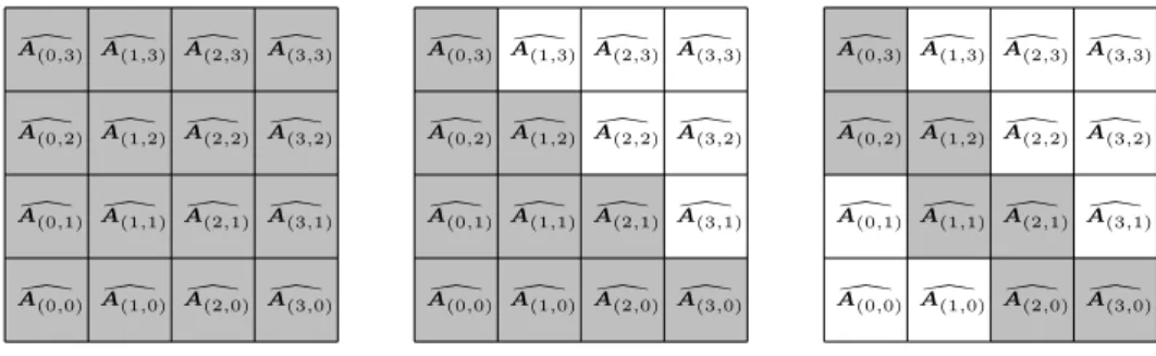
Figure 1: For discretization levelJ = 3, multilevel frames on the full tensor product space require a very densely populated system matrix AdJ (left), while sparse approximation leads to the system matrix AgJ (center) with smaller size due to fewer active (i.e. gray) matrix subblocks. The sparse grid combination technique (right)leads to the most efficient approximation. Consequently, (AJ⊗AJ) becomes a matrix of size NJ2×NJ2. Moreover,
UJ,FJ ∈RNJ·NJ are the solution and the right-hand side, respectively. By assuming an underlying d-dimensional finite element discretization with mesh width h and a multigrid-type linear solver, solving the linear system in (7) would require at least O h−2d operations, in contrast to O(h−d) for the problem given by (2). This amount of computational work is prohibitively large, especially for largerd. Therefore, we shall find a way to reduce the amount of work to solve this problem. Before we do that, we change the problem discretization to a multilevel discretization, which is the basis for the subsequent sparse approaches.
3.1 Multilevel frames for tensor product constructions
As in Section 2.1, we can forj = (j, j0) introduce multiple levels of systems of linear equations (Aj ⊗Aj0)Uj =Fj (8) with Aj =PjJAJPJj and Fj = PjJ ⊗PjJ0FJ
by applying coarsening and the transfer operators of algebraic multigrid. Thereby, we obtain
(Aj⊗Aj0)∈RNjNj0×NjNj0 and Uj,Fj ∈RNjNj0.
Pjj0 is the prolongation / restriction matrix introduced in Section 2.1. By extending the solution approach in Section 2.2 to tensor product problems, we finally obtain the multilevel frame linear system for the tensor product problem as
d
Here, we have
d
AJ = [Aj⊗Aj0]j,j0≤J =: [Acj]kjk`∞≤J,
and
UJ = [Uj]kjk`∞≤J, FJ = [Fj]kjk`∞≤J.
Note that we indeed construct frames over the tensor product problems instead of constructing a tensor product of frame discretizations, cf. [14].
In order to characterize the computational complexity for the solution of (9), we recall that we assume to have a constant operator complexity for the sequence of matrices Aj, i.e. Pη(Aj) ≤ c η(AJ). Moreover, by definition of the Kronecker product, we have the number of non-zeros in each block ofAdJ given by
η(Aj⊗Aj0) =η(Aj)η(Aj0).
From that, we can estimate the total number of non-zeros indAJ by η(dAJ) =
X
j,j0≤J
η(Aj)η(Aj0)≤c2η(AJ)2.
This means that the computational work to solve (9) is asymptotically iden-tical to a solve of (7).
3.2 Sparse tensor product construction
Solving (7) or (9) would be prohibitively expensive, cf. Figure 1. As in the geometric multilevel case, we assume that the solution of the elliptic problem (1) on Ω isHsregular. Therefore, the solution of the tensor product problem (6) becomes Hmixs -regular, see [18]. This allows to follow, for example, the lines of [14] to introduce a sparse, however now algebraically constructed, version of the discretized problem. Instead of using all sub-problems for multi-indices kjk`∞ ≤ J, the sparse approximation is reduced to multi-indiceskjk`1 ≤J. Thereby, we obtain a new system of linear equations
g
AJgUJ =gFJ with
g
AJ := [Acj]kjk`1≤J, UJ = [Uj]kjk`1≤J, FJ = [Fj]kjk`1≤J. Figure 1 compares both choices in the plots on the left-hand side and the center.
As discussed before, there is not much theory on the size of the levels in the algebraic multilevel construction. The only available information is the assumed bound on the operator complexity. However, this does not give
enough information to discuss the expected improvement in performance due to the sparse construction. Nevertheless, the bound implies a similar scaling of the non-zeros with levelj as in the geometric multilevel construc-tion. Therefore, we here briefly discuss the number of non-zeros in gAJ for the geometric construction to give a hint towards the possible performance improvement by the algebraic sparse construction.
With this in mind, we follow the previous example of (linear) finite el-ements on a mesh with mesh width h. The number of non-zero entries for matrixAj is proportional to the number of elements and therefore
η(Aj) =O(2d j). Moreover, we haveJ =O(|logh|). By evaluating
ηgAJ = X kjk`1≤J ηAcj ,
one can easily verify that the number of non-zeros in the system matrix in
g
AJ is asymptotically
ηgAJ
=O|logh|h−d.
That is, in case a BPX-type preconditioner [2, 5, 6, 16] and an optimal approach for the construction of the sub-problem matrices Acj [1, 3, 24] is used, the computational complexity of the problem on the tensor product domain Ω×Ω is (up to a logarithmic factor) reduced to the computational complexity of the problem on domain Ω.
3.3 Sparse grid combination technique
It has been shown [13] that the previous sparse approximation is equivalent to the so-called sparse grid combination technique. The latter one requires to solve a set of decoupled problems
c
AjUj =Fj, where kjk`1 ∈ {J, J −1}. (10) These are afterwards combined to a solution
d UJ = X kjk`1=J (PJj ⊗PJj0)Uj − X kjk`1=J−1 (PJj ⊗PJj0)Uj. (11)
On the right-hand side of Figure 1, the sub-matricesAcjused in this approxi-mation have been marked gray. As before, one can easily verify that the total number of non-zeros of the matrices in (10) is asymptoticallyO |logh|h−d for the case of linear finite elements on a tetrahedral mesh with mesh widthh
inddimensions and a geometrically constructed multilevel structure. How-ever, Figure (1) easily clarifies that the pre-asymptotic number of non-zeros in the matrices involved in the combination technique is much smaller than the non-zeros in the sparse approximation discussed before.
In terms of computational complexity of the combination technique, let us remind that the (approximate) solution of each sub-problem in (10) can be realized by an iterative linear solver with matrix-vector products. To be more specific, tensor product versions of standard iterative solvers can be constructed, by reshaping a given iterate Uj=(j,j0) ∈ RNj·Nj0 (and the appropriate right-hand side) to a matrix of sizeNj×Nj0. Then, the action of one step of an iterative solver for matrixAcj =Aj ⊗Aj0 is done by first applying the iterative solver step for Aj to all Nj0 columns of the reshaped matrix and by second applying the iterative solver step for Aj0 to all Nj rows of the reshaped matrix. Since we have all prolongation and restriction operators from AMG at our disposal, we can construct, in the above way, a tensor product version of algebraic multigrid. Given this solver, we ob-tain roughly problem-size independent convergence for each sub-problem in (10), i.e. we need O(NjNj0) operations for each sub-problem. In the geo-metric setting, we would again have the relation Nj = O(2dj) and thereby O(2d(j+j0)) operations per sub-problem. Since it holds kjk
`1 ∈ {J, J −1} and the number of sub-problems is O(J), we would finally end up with a computational complexity ofO(J2dJ) or O(NJlogNJ).
4
Implementation
In our numerical results, we approximate solutions for tensor product fi-nite element discretizations of elliptic problems based on the combination technique. To this end, we assemble system matrices for a given problem, construct the multilevel hierarchies, solve the decoupled, anisotropic prob-lems in (10) and combine the solutions following the combination rule (11).
Assembly of system matrices. The discretization by the finite element method is done with theMatlab PDE ToolboxofMatlab 2017a. We use linear finite elements and construct meshes with maximum element size Hmax= 2−J. Furthermore, we use the optionJiggleto optimize the mesh in quality. The stiffness matrix (incorporating boundary conditions) is constructed by using the Matlab command assembleFEMatrices with option nullspace. In a similar way, we extract the mass matrix. Afterwards, both matrices and the mesh node coordinates are stored to files.
Construction of the multilevel hierarchy. From withinMatlabwe call a newly implemented code that uses the parallel linear solver libraryhypre in version 2.11.1. This library contains the implementation BoomerAMG
of classical Ruge-St¨uben AMG. The code reads the matrix from file and creates the AMG multilevel hierarchy by usinghypre. In addition tostandard coarseningwith strength measurestr = 0.25 andstandard interpolation, we use two passes ofJacobi interpolation [21] with a truncation of the Jacobi interpolation with a threshold of 0.001 for the two-dimensional problems and 0.01 for the three-dimensional problem. All other parameters are kept as the defaults ofBoomerAMG. After having created the multigrid hierarchy, the program stores the prolongation matrices of all created levels to files. These are read by Matlab.
Solution of the anisotropic tensor product problems. Based on the prolongation matrices and the system matrix AJ on the finest levels, the decoupled problems in (10) can be set up. As discussed before, a tensor product version of AMG is used to solve the systems of linear equations. In our implementation, we construct the sub-problem operators in (10) by individually multiplying the transfer operators between two consecutive lev-els.
Our tensor product AMG is iterated until the convergence criterion kRitjk`2/kFjk`2 ≤tol
is fulfilled, whereRitj is the residual of the current iterateUitj in the solver. Since the problems in (10) completely decouple, we can easily parallelize their solution process by aparforloop inMatlab. In case an individual prob-lem becomes very expensive, we further impprob-lemented a distributed memory parallelization for the tensor product AMG based onMatlab’sdistributed
function. Thereby, we overcome the limitation of a non-existing multi-core parallelization for sparse matrix-vector products inMatlab.
Combination of the solutions. In the combination phase, we avoid to prolongate the full partial solutions to the finest level J. Instead, we ran-domly choseNeval nodes on the product of the finest meshes on Ω×Ω. On these points, we evaluate the combination formula (11) and compute the empirical error measure
e(Uapprox) =kUapprox−Urefk`2/kUrefk`2,
where Uapprox is the approximated solution and Uref is an appropriately evaluated reference solution. Note that we do not multiply the tensor prod-uct of the prolongation with the solution. However, we follow the ideas from Section 3.3 for the construction of the tensor product AMG and apply the prolongations direction-wise. The prolongation for each sub-problem is also parallelized by a parforloop.
5
Numerical results
In our empirical studies, we consider the numerical solution of the problem (∆⊗∆)u=f on Ω×Ω,
u= 0 on ∂(Ω×Ω). (12) by means of the combination technique based on the algebraic multilevel hierarchy. Different choices will be made for the domain Ω and the right-hand sidef.
5.1 Analytic example on a disk
The first study is done on a disk domain Ω with center (0,0)> and radius 0.5. We set
f(x,y) = 1. The exact solution of the resulting problem is
u(x,y) = 1 16 x 2 1+x22−0.52 y21+y22−0.52 .
To approximate the solutionuby the combination technique, we follow the methodology discussed in Section 4. As part of this, we triangulate the geometry with a maximum element width of 2−J. Figure 2 shows on the left-hand side the resulting mesh forJ = 5. It is obvious that the resulting mesh is unstructured. Therefore, classical geometric constructions for the sparse grid combination technique would not be feasible on that mesh. In contrast, our new algebraic approach can solve this problem.
This is shown on the right-hand side of Figure 2, where we compare the numerically approximated solution against the above exact solution. Con-vergence results for the choices J = 3, . . . ,8 are given. From literature, compare e.g. [13], we know that the error of the geometrically constructed sparse grid combination technique scales for the problem under consideration likeJ4−J. As we can see from the convergence results in Figure 2, the al-gebraically constructed combination technique shows the same convergence behavior, while being applicable to unstructured grids.
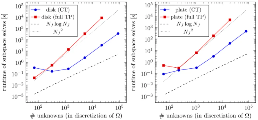
Figure 3 shows on the left-hand side computing times for growing prob-lem size NJ of the univariate discretization of Ω. We compare the time required for the solution of the combination technique sub-problems with the time required to solve the full product problem (7) by our tensor-product AMG implementation. Note that we use the coarse grid hieararchies reported in Table 1 for both the combination technique and the full tensor-product approach. All measurements were done on a compute server with dual 20-core Intel Xeon E5-2698 v4 CPU at 2.2 GHz and 768 GB RAM. It becomes evident that our algebraically constructed combination technique
3 4 5 6 7 8 10−3 10−2 10−1 levelJ relativ e ` 2error e ( Uexact ) error J4−J
Figure 2: The combination technique based on our algebraic multilevel hi-erarchy and applied to the tensor product of a disk geometry with an un-structured mesh (left, triangulated with J = 5) shows the same convergence as the geometrically constructed combination technique (right).
approach beats the full tensor-product approach in both, computational complexity and effective runtime. However, both results do not show the predicted computational complexity of O(NJlogNJ) and O(NJ2). There are several reasons for this behavior.
• First, algebraic multigrid often shows a small, roughly logarithmic, growth in the number of iterations for larger problem sizes, resulting in a slow-down by a logarithmic factor.
• Second, we observe a certain fill-in in the system matrices for coarser problems in the algebraic construction due to our choice of an ad-ditional (truncated) Jacobi interpolation. However, this should be pre-asymptotic behavior.
• Third, as can be seen in Table 1, the AMG coarsening approach chosen in our implementation does not show the exact same decay rate in the number of levels as we expect from the geometric construction. In fact, this leads to a problem-size dependent growth of the coarsest grid. While this growth does not affect the error decay, it shows up in the computational complexity.
Meanwhile, as stated before, we are able to beat the solution approach based on the full tensor-product approach in terms of computational complexity. Even more, in terms of runtime, we are by more than two orders of magni-tude faster.
102 103 104 105 10−3 10−2 10−1 100 101 102 103 104 105
# unknowns (in discretiztion of Ω)
run time of subspace solv es [s] disk (CT) disk (full TP) NJlogNJ NJ2 102 103 104 105 10−3 10−2 10−1 100 101 102 103 104 105
# unknowns (in discretiztion of Ω)
run time of subspace solv es [s] plate (CT) plate (full TP) NJlogNJ NJ2
Figure 3: We compare the runtime of the new combination technique ap-proach (CT) with the runtime of the traditional the full tensor-product approach (full TP) for the solution of the tensor product elliptic problems on the disk geometry(left) and the plate geometry(right).
# dofs on algebraically coarsened levelj
Ω J\j 0 1 2 3 4 5 6 7 8 9 disk 3 3 11 28 71 4 8 21 52 119 320 5 12 31 84 207 495 1292 6 20 51 139 348 852 2009 5234 7 35 93 244 606 1473 3510 8415 22118 8 46 130 366 978 2469 5983 14480 34081 89097 plate 3 5 20 61 4 16 36 90 230 5 28 68 168 414 1072 6 46 116 297 745 1813 4703 7 63 184 515 1272 3117 7491 19611 8 103 302 815 2124 5301 12822 30639 80146 spanner 3 4 10 19 50 117 247 4 11 22 59 147 326 689 1454 5 40 114 300 689 1516 3216 6484 13939 6 210 548 1364 3123 6708 14109 29103 57438 125223 7 1386 3120 6627 14016 29533 61150 124921 253291 496614 1082581
Table 1: For a given problem on levelJ, the algebraic multilevel construction on our example domains Ω constructs coarser levels with a decrease of the number of unknowns roughly similar to geometric multilevel constructions. Above, only those levels j are reported that are used in the convergence study.
3 4 5 6 7 8 10−3 10−2 10−1 100 levelJ relativ e ` 2error e ( Uappr ox ) error J4−J
Figure 4: Even for a covariance load on a complex geometry (left, triangu-lated for J = 5), the algebraic construction shows the appropriate conver-gence rate after a short pre-asymptotic phase(right).
5.2 Example on complex geometry with covariance load
The next numerical study is concerned with the solution of the problem (12) with the load
f(x,y) = exp
−kx−yk2
`
that corresponds to an (unscaled) Gaussian covariance kernel with corre-lation length `. This is a prototype version of the tensor product elliptic problem on Ω×Ω showing up in the computation of the output covariance of an elliptic problem on Ω with random input, cf. [14].
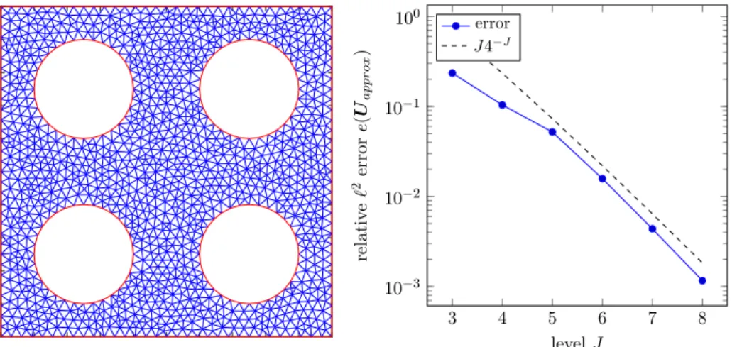
In addition to the more complicated right-hand side, we solve the prob-lem for a rather complex geometry Ω. We choose the geomery of a square plate on [0,1]2 with circular wholes of radius 0.15 which are centered at the
points
{(0.25,0.25),(0.25,0.75),(0.75,0.25),(0.75,0.75)}.
Figure 4 shows its triangulation for J = 5 on the left-hand side. Note that it would be almost impossible to solve a problem on such a geometry with the geometrical construction for the sparse grid combination technique. However, with the algebraic construction, a coarsening to very few degrees of freedom becomes easily possible, compare Table 1.
To be able to compare the above problem against a numerically com-puted reference solution, we replace the (sampled) covariance kernel for`= 1 by its low-rank approximation computed with the pivoted Cholesky factor-ization [12], truncated for a trace norm of 10−8. In this case, depending on
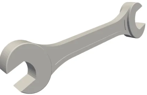
Figure 5: In our large-scale real world example, we solve an elliptic problem on the tensor product of the three-dimensional geometry of a spanner. For a discretization level ofJ = 7, the discretization of Ω has more than a million unknowns. This would lead to 1012, that is a trillion, unknowns in the full tensor product discretization.
On the right-hand side of Figure 4, we show the convergence results with errors computed against the numerically approximated exact solution by use of the low-rank approximation. After a pre-asymptotic phase, we are able to attain an error that scales likeJ4−J as in the geometric construction.
The problem size dependent runtime to compute the subspace solutions for the plate geometry is given in Figure 3 on the right-hand side. We observe similar compuational complexities and similar runtimes as in the previous example on the disk.
5.3 Large-scale real-world example
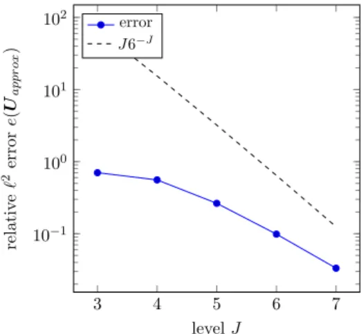
Our last numerical study treats a large-scale problem with a complex real-world geometry Ω. We again aim at solving (12) forf(x,y) = 1. However, we choose the three-dimensional spanner geometry found in Figure 5. In contrast to the previous examples, we set the maximum mesh width to 25−J, since the geometry is contained in the rather large bounding box [−5,5]× [−12.2,112]×[−15.7,15.7]. Note that the triangulation of Ω results for level J = 7 in a discretization with 1,082,581 unknowns. That is, if we would want to solve the full tensor product problem on Ω×Ω, cf. (6), then we would have to solve a problem with about 1012, that is a trilion, unknowns. This
3 4 5 6 7 10−1 100 101 102 levelJ relativ e ` 2error e ( Uappr ox ) error J6−J
Figure 6: Our algebraic multilevel construction for the sparse grid com-bination technique on the large-scale three-dimensional spanner geometry gradually approaches the optimal convergence rate ofJ2−dJ.
would be clearly out of scope even for large parallel clusters. In contrast, the combination technique allows to solve this problem. Nevertheless, we still have to solve, e.g. for levelJ = 7 and the system matrix \A(0,J) a problem with 1,082,581×1,386 unknowns, compare Table 1.
In Figure 6, we show the convergence results for this large scale problem relative to a numerical approximation of the solution. Due to the high dimensionality and complexity of the domain Ω, the convergence results in Figure 6 are only gradually approaching the optimal scaling of J2−dJ. Nevertheless, we are able to solve this problem up to a certain accuracy. This shows that even very complex problems of large scale can be solved by the proposed approach.
6
Conclusions
In this work, we have introduced an algebraic construction method for the sparse approximation of tensor product elliptic problems by means of the combination technique. While previous approaches were tight to geometric hierarchies of mesh refinements to build the underlying multilevel discretiza-tion, we were able to solve the given type of problems on complex geometries and for unstructured grids by an algebraic multilevel hieararchy based on AMG. We could show that our approach has the same convergence rates as the geometric construction. Measurements of the computational complexity were in the linear range with poly-logarithmic factors. Overall, we are now able to apply sparse approximation for elliptic tensor product problems in a black-box fashion.
References
[1] R. Balder and C. Zenger. The solution of multidimensional real Helmholtz equations on sparse grids. SIAM Journal on Scientific Com-puting, 17(3):631–646, 1996.
[2] J. Bramble, J. Pasciak, and J. Xu. Parallel multilevel preconditioners. Mathematics of Computation, 55:1–22, 1990.
[3] H.-J. Bungartz. A multigrid algorithm for higher order finite elements on sparse grids.ETNA. Electronic Transactions on Numerical Analysis, 6:63–77, 1997.
[4] H.-J. Bungartz and M. Griebel. Sparse grids.Acta Numerica, 13:1–123, 2004.
[5] W. Dahmen. Wavelet and multiscale methods for operator equations. Acta Numerica, 6:55–228, 1997.
[6] M. Griebel. Multilevelmethoden als Iterationsverfahren ¨uber Erzeugen-densystemen. Teubner Skripten zur Numerik. B.G. Teubner, Stuttgart, 1993.
[7] M. Griebel. Multilevel algorithms considered as iterative methods on semidefinite systems. SIAM International Journal Scientific Statistical Computing, 15(3):547–565, 1994.
[8] M. Griebel and H. Harbrecht. On the convergence of the combination technique. In J. Garcke and D. Pfl¨uger, editors,Sparse grids and Appli-cations – Stuttgart 2014, volume 97 ofLecture Notes in Computational Science and Engineering, pages 55–74. Springer, 2014.
[9] M. Griebel and P. Oswald. Greedy and randomized versions of the multiplicative Schwarz method. Linear Algebra and its Applications, 7:1596–1610, 2012.
[10] M. Griebel, M. Schneider, and C. Zenger. A combination technique for the solution of sparse grid problems. In P. de Groen and R. Beauwens, editors, Iterative Methods in Linear Algebra, pages 263–281. IMACS, Elsevier, North Holland, 1992.
[11] H. Harbrecht. A finite element method for elliptic problems with stochastic input data. Applied Numerical Mathematics, 60(3):227–244, Mar. 2010.
[12] H. Harbrecht, M. Peters, and R. Schneider. On the low-rank approx-imation by the pivoted Cholesky decomposition. Applied Numerical Mathematics, 62(4):428–440, 2012.
[13] H. Harbrecht, M. Peters, and M. Siebenmorgen. Combination technique basedk-th moment analysis of elliptic problems with random diffusion. Journal of Computational Physics, 252(C):128–141, Nov. 2013.
[14] H. Harbrecht, R. Schneider, and C. Schwab. Multilevel frames for sparse tensor product spaces. Numerische Mathematik, 110(2):199–220, July 2008.
[15] M. Hegland, J. Garcke, and V. Challis. The combination technique and some generalisations. Linear Algebra and its Applications, 420(2):249– 275, 2007.
[16] P. Oswald. Multilevel finite element approximation. Theory and ap-plications. Teubner Skripten zur Numerik. B.G. Teubner, Stuttgart, 1994.
[17] J. Ruge and K. St¨uben. Algebraic multigrid (AMG). In S. McCormick, editor,Multigrid Methods, Frontiers in Applied Mathematics, volume 5. SIAM, Philadelphia, 1986.
[18] C. Schwab and R. A. Todor. Sparse finite elements for elliptic problems with stochastic loading. Numerische Mathematik, 95(4):707–734, 2003. [19] C. Schwab and R. A. Todor. Sparse finite elements for stochastic elliptic problems: Higher order moments. Computing, 71(1):43–63, Sept. 2003. [20] K. St¨uben. A review of algebraic multigrid. Journal of Computational and Applied Mathematics, 128(12):281–309, 2001. Numerical Analysis 2000. Vol. VII: Partial Differential Equations.
[21] U. Trottenberg and A. Schuller. Multigrid. Academic Press, Inc., Or-lando, FL, USA, 2001.
[22] U. M. Yang. On long-range interpolation operators for aggressive coars-ening. Numerical Linear Algebra with Applications, 17(2-3):453–472, 2010.
[23] P. Zaspel. Subspace correction methods in algebraic multi-level frames. Linear Algebra and its Applications, 488:505–521, 2016.
[24] A. Zeiser. Fast matrix-vector multiplication in the sparse-grid Galerkin method. SIAM Journal of Scientific Computing, 47(3):328–346, 2011.
LATEST PREPRINTS
No.
Author:
Title
2016-30
W. D. Brownawell, D. W. Masser
Unlikely intersections for curves in additive groups over positive
characteristic
2016-31
M. Dambrine, H. Harbrecht, M. D. Peters, B. Puig
On Bernoulli's free boundary problem with a random boundary
2016-32
H. Harbrecht, J. Tausch
A fast sparse grid based space-time boundary element method for the
nonstationary heat equation
2016-33
S. Iula
A note on the Moser-Trudinger inequality in Sobolev-Slobodeckij spaces in
dimension one
2016-34
C. Bürli, H. Harbrecht, P. Odermatt, S. Sayasone, N. Chitnis
Mathematical analysis of the transmission dynamics of the liver fluke,
Opisthorchis viverrini
2017-01
J. Dölz and T. Gerig, M. Lüthi, H. Harbrecht and T. Vetter
Efficient computation of low-rank Gaussian process models for surface and
image registration
2017-02
M. J. Grote, M. Mehlin, S. A. Sauter
Convergence analysis of energy conserving explicit local time-stepping
methods for the wave equation
2017-03
Y. Bilu, F. Luca, D. Masser
Collinear CM-points
2017-04
P. Zaspel
Ensemble Kalman filters for reliability estimation in perfusion inference
2017-05
J. Dölz and H. Harbrecht
Hierarchical Matrix Approximation for the Uncertainty Quantification of
Potentials on Random Domains
2017-06
P. Zaspel
Analysis and parallelization strategies for Ruge-Stüben AMG on many-core
processor
2017-07
H. Harbrecht and M. Schmidlin
Multilevel Methods for Uncertainty Quantification of Elliptic PDEs with
Random Anisotropic Diffusion
LATEST PREPRINTS
No.
Author:
Title
2017-08
M. Griebel and H. Harbrecht
Singular value decomposition versus sparse grids: Refined complexity
Estimates
2017-09
J. Garcke and I. Kalmykov
Efficient Higher Order Time Discretization Schemes for
Hamilton-Jacobi-Bellman Equations Based on Diagonally Implicit Symplectic Runge-Kutta
Methods
2017-10
M. J. Grote and U. Nahum
Adaptive Eigenspace Regularization For Inverse Scattering Problems
2017-11
J. Dölz, H. Harbrecht, S. Kurz, S. Schöps and F. Wolf
A Fast Isogeometric BEM for the Three Dimensional Laplace- and
Helmholtz Problems
2017-12
P. Zaspel
Algorithmic patterns for
H
-matrices on many-core processors
2017-13
R. Brügger, R. Croce and H. Harbrecht
Solving a free boundary problem with non-constant coefficients
2017-14
M. Dambrine, H. Harbrecht and B. Puig
Incorporating knowledge on the measurement noise in electrical impedance
tomography
2017-15
C. Bürli, H. Harbrecht, P. Odermatt, S. Sayasone and N. Chitnis
Analysis of Interventions against the Liver Fluke, Opisthorchis viverrini
2017-16
D. W. Masser
Abcological anecdotes
2017-17
P. Corvaja, D. W. Masser and U. Zannier
Torsion hypersurfaces on abelian schemes and Betti coordinates
2017-18
F. Caubet, M. Dambrine and H. Harbrecht
A Newton method for the data completion problem and application
to obstacle detection in Electrical Impedance Tomography
2018-01
H. Harbrecht and P. Zaspel
On the algebraic construction of sparse multilevel approximations of elliptic
tensor product problems